Applications of Boundary Node Method to Simulation of Piezoelectric Composites

(1)

18th International Conference on Structural Mechanics in Reactor Technology (SMiRT 18) Beijing, China, August 7-12, 2005 SMiRT18-B01-8

APPLICATIONS OF BOUNDARY NODE METHOD TO SIMULATION OF

PIEZOELECTRIC COMPOSITES

Guowen Tan

1)

Phone: +86-10-62778962

Fax: +86-10-62781824

Song Cen

1,2)

Phone: +86-10-62772935

Fax: +86-10-62781824

Hongtao Wang

1)

Phone: +86-10-62778962

Fax: +86-10-62781824

* Zhenhan Yao

1,2)

Phone: 86-10-62772913

Fax: +86-10-62781824

Dept. of Engineering Mechanics

，

Tsinghua Univ., Beijing 100084, China

2)

Failure Mechanics Laboratory, Tsinghua University, Beijing, 100084, China

ABSTRACT

As a type of boundary-only meshless method, boundary node method (BNM) combines the Moving Least Square (MLS) approximation and the regularized boundary integral equation (BIE) and inherently possesses the attractive advantages of both the boundary element method (BEM) and meshless method. In this paper, by the combination of the BNM and the repeated similar sub-domain approach, a scheme for the 2-D simulation of piezoelectric composites is presented. Moreover, the micromechanics algorithm is applied to determine the effective electroelastic properties of transversely isotropic piezoelectric materials containing randomly distributed inclusions. These 2-D analyses based on fundamental solutions are carried out to investigate the relations between the effective properties and the inclusion volume fraction. Emphasis is placed on the application of the scheme of repeated similar sub-domain BNM to obtain the coupled elastic and electric fields by discretizing the outer boundaries and the inner matrix-inclusion interfaces of the entire physical domain and further to numerically determine the effective properties of piezoelectric composites. The numerical results illustrate great agreement with the available exact solution and the analytical predictions by Mori-Tanaka model.

Keywords: Effective properties; Boundary node method; Piezoelectric material; Inclusions; Repeated similar sub-domain

1. INTRODUCTION

With the rapid development of intelligent and smart structures, micro-electro-mechanical systems (MEMS), piezoelectric materials have been widely used as sensors and actuators in many engineering fields. In processing of piezoelectric materials, all kinds of defects, cracks, voids or inclusions inevitably occur within the structures. Changes of the overall properties of a piezoelectric material due to the presence of voids or inclusions considerably affect the functions of piezoelectric smart structures as well as MEMS. Micromechanical analyses of piezoelectric structures for integrity and actualizations of a certain special function require the knowledge about the influences of voids or inclusions on the effective properties of piezoelectric materials. Therefore, investigations of the effective properties of a piezoelectric material containing defects are of scientific significance and engineering importance [1, 5, 8].

(2)

provide an approximate evaluation of the overall properties of piezoelectric materials based on the assumption of average over the studied physical domain. For instance, Wu [7] adopted the equivalent inclusion method [19] and Mori and Tanaka’s mean field theory [6] to evaluate the influences of void volume fraction and the void shape on the electroelastic properties of piezoelectric materials. Dunn et al. [24] presents a theoretical approach to predict the electromechanical properties of porous piezoelectric ceramics. This analysis is able to account for the effects of porosity shape and concentration and is applicable to piezoelectric material of arbitrary symmetry.

Some efforts have also been made in recent years to numerically simulate piezoelectric materials and determinate the effective properties. Li et al. [5] studied the effective properties by FEM using ANSYS, based on a cubic unit cell model. As mentioned in [5], that kind of cell analysis is only suitable to periodical distributed voids. Lee [15] and Liu et al. [18] analyze piezoelectric materials with a defect by BEM. Qin [1] proposed a micromechanics BE algorithm for analyzing the overall properties of piezoelectric material with cracks or voids of various shapes. In [1], numerical results of effective material constants are obtained by self-consistent BE method with an iterative scheme and Mori-Tanaka-BEM approach.

Most progress has been made in determination of the overall properties of piezoelectric materials containing defects of regular shapes [1, 6-8, 22-25]. In practical applications of piezoelectric materials, however, it is very likely that defects are of high shape irregularity. Therefore, overall analysis of a piezoelectric structure using finite element method may suffer from difficulties due to a large number of defects with irregular shapes and fine mesh required locally. In recent years, several boundary-only meshless methods, based on meshless interpolation schemes such as Moving Least Square (MLS) approximation, have been proposed to avoid these drawbacks [12-14]. These methods include Boundary Node Method [12], Boundary Point Interpolation Method (BPIM) [13], and Hybrid Boundary Node Method [14], et al. In this paper, the BNM is adopted.

In the BNM, the MLS approximation is introduced into the regularized BIE, and only some scattered nodes distributed on the boundary are required. Thus, the BNM possesses the meshless character of MLS as well as the dimension-reduction advantage of BEM, which reduce even eliminate the difficulties in problems involving frequent re-meshing, such as crack propagation.

In this paper, based on the idea of the BEM scheme for the determination of effective elastic properties presented by the authors’ group [10, 11], a BNM scheme for evaluating the effective properties of piezoelectric composites is proposed. This BNM scheme simulates the structure of piezoelectricity by fully descretizing the outer boundaries and the inner matrix-inclusion interfaces of the entire physical domain and produces high accurate results. This scheme is a promising approach for analyzing composite materials with a large number of defects/inclusions of both regular and irregular shapes.

2. GOVERNING EQUATIONS IN PIEZOELECTRICITY

The theory of piezoelasticity is summarized in this section. The basic governing field equations are [9, 16, 18, 20, 21]

,

0

ij j

f

i

σ

+ =

(1)

,

0

i i

D

− =

q

(2)

where

σ

ijis the stress tensor,

f

ithe body force vector per unit volume,

D

ithe electric displacement vector and

q

is the electric charge per unit volume. Eq. (1) is the equilibrium equation of elasticity and the Eq. (2) the Gauss’s law of electrostatics. Consider a piezoelectric material the constitutive relation is formulated as

ij

C

ijkl kl

e E

kij k

σ

=

ε

−

(3)

i ikl kl ik k

D

=

e

ε

+

κ

E

(4)

where

ε

_klis the elastic strain tensor,

E

_kthe electric field vector,

C

_ijkl the elastic modulus tensor measured in a constant electric field,

e

_ijkthe piezoelectric tensor and

κ

_ijthe dielectric tensor measured at constant strains. The elastic strain field

ε

_ij and electric field

E

_iare defined by

, ,

1 (

)

2

ij

u

i j

u

j i

ε

=

+

(5)

, i i

E

= −

φ

(6)

(3)

mechanical boundary conditions:

on

i

ij j i t

i i u

n

t

u

σ

=

Γ

⎧⎪

⎨ =

Γ

⎪⎩

(7)

electric boundary conditions:

on

i i

D n

_ω

φ

ω

φ φ

= −

Γ

⎧⎪

⎨ =

Γ

⎪⎩

(8)

where

t

_i and

ω

are the traction and the surface charge respectively, and

n

_ithe unit outward normal vector of the surface. The upper-barred quantities indicate prescribed values. Note that

i i

t u ω φ

Γ

∪

Γ = Γ

∪

Γ = Γ

, and

i i

t u ω φ

Γ

∩

Γ = Γ

∩

Γ = ∅

.

If the displacement

u

_i and the electric potential

φ

are independent of

x

₂, the problem reduces to plane-strain case. For a transversely isotropic piezoelectric material with the

x

₃ being the axis of poling direction and let

x

₁−

x

₃ plane be the plane of interest. The constitutive Eqs. (3) and (4) reduce to the following matrix equations

11 11 13 31 11

33 13 33 33 33

31 44 15 31

1 15 11 1

3 31 33 33 3

0

2

0

0 C

C

e

C

e

C

e

D

e

E

D

e

E

σ

ε

σ

ε

σ

ε

κ

−

⎧

⎫ ⎡

⎤ ⎧

⎫

⎪

⎪ ⎢

₋

⎥ ⎪

⎪

⎪ ⎢

⎥ ⎪

⎪

₌

_⎢

₋

_⎥

⎪

⎨

⎬

⎨

⎬

⎢

⎥

⎪

⎢

⎥

⎪

⎢

⎥

⎪

⎩

⎭ ⎣

⎦ ⎩

⎭

(9)

3. MOVING LEAST SQUARE (MLS) APPROXIMATION

In this paper, the MLS approximations are constructed along the piecewise smooth segments

,

1, 2,

,

k

M

Γ

=

independently, in curvilinear coordinates. The approximation scheme for the boundary displacement

u

_i and boundary traction

t

_i are independently defined as

1

ˆ

( )

N I I i i I

u s

s u

=

∑

Φ

(10)

1

ˆ

( )

N I I i i I

t s

s t

=

∑

Φ

(11)

where 1 1

( )

( ) ( )

m _jI I j j

s

p s

−

s

=

⎡

⎤

Φ

=

∑

_⎣

A

B

_⎦

(12)

T 1

( )

( ) (

)

(

)

N

I I I

I

s

w s

s

=

∑

A

p

(13)

1 1 2 2

( )

s

= ⎣

⎡

w s

( ) ( ),

s

w s

( ) (

s

),

w

N

( ) (

s

N

)

⎤

_⎦

B

p

(14)

In the above equations,

p

is a complete monomial basis vector and

w s

I

( )

is the weight function. In this paper, the Gaussian weight function is chosen as

2 2

2

ˆ

exp[ (

/

) ] exp[ (

/

) ]

_ˆ

0 ˆ

( )

1 exp[ (

/

) ]

ˆ

0

I I I I

I I

I I I

I I

d

c

d

c

d

w s

d

c

d

⎧

₋

≤

⎪

=

_⎨

−

⎪

_≥

⎩

(15)

where

d

I is the distance from a point

s

to the boundary node

s

I measured along

Γ

k,

d

ˆ

I the support size of the weight function and

c

I is the parameter controlling the shape of the weight function.

(4)

fictitious nodal values and

u

_iI and

t

_iI are the exact nodal values. For a well-posed problem, the value of either

u

_i or

t

_i is known on the boundary. Therefore,

u

ˆ

_iI and

t

ˆ

_iIcan be obtained first

1 1

ˆ

N N

I IJ J IJ J

i i i

J J

u

R u

= =

=

∑

=

∑

(16)

1 1

ˆ

N N

I IJ J IJ J

i i i

J J

t

R t

= =

=

∑

=

∑

(17)

where

1

(

)

IJ J I

R

= Φ

⎡

_⎣

s

⎤

_⎦

− ;

N

is the total number of the boundary nodes on the edge

Γ

k.

4. BOUNDARY NODE METHOD FOR 2-D PIEZOELECTRICITY

The regularized form of the BIE for 2-D piezoelectricity without body force and electric charge can be written as [18]

[

]

( , )

P q

( )

q

( ) d ( )

P

q

( , ) ( )d ( )

P q

q

Γ

−

Γ

=

Γ

∫

T

u

∫

U

t

(18)

where

* * *

1 1 1 1 11 12 13 11 13 1

* * *

2 3 2 3 21 22 23 31 33 3

* * *

3 3 31 32 33 41 43 4

11 12 13 21 22 23 31 32 33

,

u

t

U

u

t

U

u

t

U

T

φ

ω

φ

⎡

⎤

⎧ ⎫

⎧ ⎫ ⎧ ⎫

⎧

⎫

⎡

⎤

⎢

⎥

⎪ ⎪ ⎪ ⎪

⎪ ⎪ ⎪

⎪

⎢

⎥

=

_{⎨ ⎬ ⎨ ⎬}

=

_{⎨ ⎬ ⎨}

=

_⎬

=

_⎢

_⎥

=

_⎢

_⎥

⎪ ⎪ ⎪ ⎪

₋

⎪ ⎪ ⎪

₋

⎪

_⎢

_⎥

_⎢

_⎥

⎩ ⎭ ⎩ ⎭

⎩ ⎭

⎩

⎭

⎣

⎦

⎣

⎦

⎡

⎤

⎢

⎥

= ⎢

⎢⎣

⎦

u

t

U

T

* * *

11 13 1

* * *

13 33 3

* * *

41 43 4

T

ω

⎡

⎤

⎢

⎥

= ⎢

⎥

⎢

⎥

⎥ ⎣

⎦

(19)

In the above equations,

P

and

q

denotes the source point and field point, respectively.

P q

,

∈ Γ

.

u

and

t

are boundary displacement and traction, respectively.

U

( , )

P q

and

T

( , )

P q

are the fundamental solutions for 2-D piezoelectricity. In this paper, we adopted the fundamental solutions which have been defined in [16, 17]:

By substituting Eqs. (10) and (11) into Eq. (18), one can obtain

1 1 1

ˆ

( , )

( )

d ( )

( , )

( ) d ( )

q P q

N N N

I I I I I I

ij j j ij j

I I I

T P q

q u

P u

q

U

P q

q t

q

Γ Γ = = =

⎡

⎤

Φ

−

Φ

Γ

=

Φ

Γ

⎢

⎥

⎢

⎥

⎣

∑

⎦

∑

∫

(20)

where

N

_P and

N

_q are the numbers of the nodes in the support of the evaluation points

P

and

q

, respectively.

The regular integrals and weakly singular integrals in Eq. (20) are evaluated by standard Gaussian quadrature and log-weighted Gaussian quadrature, respectively [26].

5. A SCHEME OF REPEATED SIMILAR SUB-DOMAIN BNM FOR 2-D PIEZOELECTRIC COMPOSITES

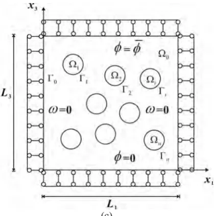
The model of 2D piezoelectric matrix with randomly distributed piezoelectric inclusions is shown in Fig. 1, in which

Ω

₀ denotes the sub-domain of the matrix,

Ω =

_i

(

i

1, 2,

, )

n

the sub-domain of the i-th inclusion,

i

Γ

the matrix-inclusion interface of the i-th inclusion, and

Γ

₀ the outer boundary of the matrix.

(5)

1

11 12 13 13 13

1

21 22 23 23 23

1

1 1 11 1 1

31 32 33 33 33

1

31 32 33 33 33

1

31 32 33 33 33

i n

i

i i i ii in

n

n n n ni nn

⎡

⎤ ⎧ ⎫

⎢

⎥ ⎪ ⎪

⎢

⎥ ⎪ ⎪

⎢

⎥ ⎪ ⎪

⎢

⎥ ⎪ ⎪

⎨ ⎬

⎢

⎥

⎪

⎢

⎥

⎪

⎢

⎥

⎪

⎢

⎥

⎪

⎢

_{⎥ ⎩ ⎭}

⎣

⎦

u

T

t

T

u

T

u

T

u

T

11 12 21 22 1 1 31 32 31 32 31 32 i i n n

⎡

⎤

⎢

⎥

⎢

⎥

⎢

⎥

⎧ ⎫

⎢

⎥

=

_⎢

_⎥

_{⎨ ⎬}

⎩ ⎭

⎪ ⎢

⎥

⎪ ⎢

⎥

⎪ ⎢

⎥

⎪ ⎢

_⎣

⎥

_⎦

U

t

u

U

(21) where

( )

1 13 13 13

1 23 23 23

1 33 33 33

i i i i i

Inc Inc

i i i i i

Inc Inc ij ij ij i i

Inc Inc − − −

⎧

₌

₊

⎪

₌

₊

⎨

⎪

=

+

⎩

T

U

T

U

T

U

T

(22)

The first and the second subscripts in Eq. (21) indicate the boundary where the source point

P

and the field point

q

locate, and 1, 2, 3 denote the known traction and displacement of the outer and interface boundaries, respectively. To distinguish different inner boundaries, the superscripts are used in the above equations. The first and the second (if applicable) superscripts indicate the number of inner boundary where the source point

P

and the field point

q

locate.

In Eq. (21),

u

stands for the unknown displacement on the outer boundary,

t

the unknown traction on the outer boundary, and

u

i the unknown displacement on the i-th interface boundary. On the other hand,

t

and

u

denote the known traction vector and the given displacement vector on the outer boundary, respectively. Matrices

U

i_Inc and

T

_Inci in Eq. (22) are coefficient matrices for the inclusion material sub-domains. Since all the randomly distributed circular inclusions are identical, the corresponding coefficient matrices

U

i_Inc and

i Inc

T

are also identical, it requires to form such coefficient matrices only once, for one inclusion.

6. COMPUTATION OF EFFECTIVE MATERIAL PROPERTIES

According to the constitutive Eq. (9) of transversely isotropic piezoelectric materials, the material constants can be obtained by imposing appropriate boundary conditions [5]. In this paper, we carry out the calculations for the effective elastic constants

C

₁₁eff

,

C

₁₃eff

,

C

₃₃eff, piezoelectric constants

e

eff₃₁

,

e

eff₃₃, and dielectric constant

κ

eff₃₃. For example, applying the boundary conditions shown in Fig. 1(a) we have

ε

₃₃

=

0

and

E

₃

=

0

. Then, we can obtain the longitudinal stiffness constant

C

₁₁eff and

C

₁₃eff

1 1

1 3

eff 11 11

11 1 1

/

x L

t d

L

C

u

L

σ

ε

=

⋅ Γ

=

∫

(23)

3 3

3 1

eff 33 13

11 1 1

/

x L

t

d

L

C

u

L

σ

ε

=

⋅ Γ

=

∫

(24)

(6)

3 3

3 1

eff 33 33

33 3 3

/

x L

t

d

L

C

u

L

σ

ε

=

⋅ Γ

=

∫

(25)

where

t

₃ is the unknown traction along the edge

x

₃

=

L

₃.

The other material constants

e

₃₁eff ,

e

₃₃eff , and

κ

₃₃eff can be obtained by imposing boundary conditions described in Fig. 1(c). They can be expressed as

1 1

1 3

eff 11 31

3 3

/

x L

t d

L

e

E

L

σ

φ

=

⋅ Γ

= −

=

∫

(26)

3 3

3 1

eff 33 33

3 3

/

x L

t

d

L

e

E

L

σ

φ

=

⋅ Γ

= −

=

∫

(27)

3 3

1 eff 3

33

3 3

/

x L

d

L

D

E

L

ω

κ

φ

=

⋅ Γ

=

∫

(28)

where

ω

is the unknown surface charge on the edge

x

₃

=

L

₃.

(7)

(c)

Fig. 1. Computational models to evaluate the effective properties

(a)

eff

11

C

and

C

₁₃eff

;

(b)

eff 33

C

; (c)

e

₃₁eff ,

e

₃₃eff

and

κ

₃₃eff .

7. NUMERICAL EXAMPLES

In this section, we present three numerical examples in which PZT-4 and PZT-6B ceramics are specified and their mechanical and electric constants are [16, 28]:

11 13 33 44

2 2 2

15 31 33

9 2 2 9 2 2

11 33

11 13 33 44

15

PZT-4:

126.0 GPa,

74.3 GPa,

115 GPa,

25.6 GPa

12.7 C/m ,

5.2 C/m ,

15.1 C/m

6.4635587 10

C /Nm ,

5.62241065 10

C /Nm

PZT-6B:

168.0 GPa,

60.0 GPa,

163.0 GPa,

27.1 GPa

C

e

C

e

κ

−

κ

−

=

= −

=

×

=

×

=

2 2 2

31 33

9 2 2 9 2 2

11 33

4.6 C/m ,

0.9 C/m ,

7.1 C/m

3.6 10

C /Nm ,

3.4 10

C /Nm

e

κ

−

κ

−

=

= −

=

×

=

×

In all examples below, the parameters in MLS approximations are chosen as

d

ˆ

I

=

3.5 h

,

d

ˆ

I

c

I

=

4.0

, in which

h

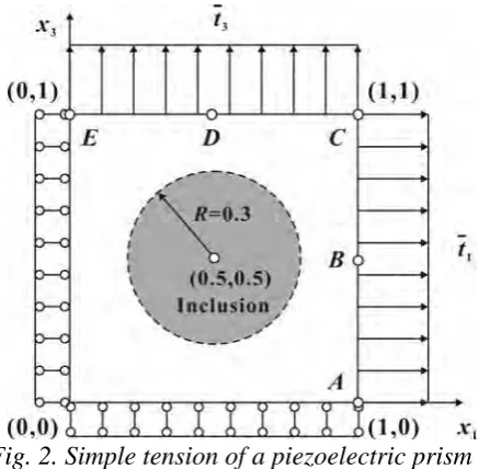
is the mesh size.

(8)

Fig. 2. Simple tension of a piezoelectric prism

A virtual inclusion is located at the center of the piezoelectric prism, with the material properties specified the same as the ones of the matrix. In this example, the PZT-4 is selected. A regular nodes scheme of 6 nodes on each edge and 20 nodes on the inner boundary of the circular inclusion are adopted. The boundary conditions are

2

1 3 1

3 1 3

0.0 m,

0.0 Pa,

0.0 C/m

when 0.0 m

0.0 m,

0.0 Pa,

0.0 V

when 0.0 m

u

t

x

u

t

x

ω

φ

⎧ =

=

⎨

=

⎩

and

2

1 3 1

2

3 1 3

10.0 Pa,

0.0 Pa,

0.0 C/m

when 1.0 m

10.0 Pa,

0.0 Pa,

0.0 C/m

when 1.0 m

t

x

t

x

ω

⎧ =

=

⎨

₌

⎩

The exact solutions obtained by the similar procedure proposed in [16] are

3 3 3

1 1 3 1 3 2 3

1 1 1

,

i i i i i i i

i i i

u

a x

u

α

a s x

φ

α

a s x

= = =

=

∑

= −

∑

= −

∑

where

2 3 3 2 3 2 2 3

1 12 13 12 13 11 13 11 13

3 1 1 3 1 3 3 1

1 3

2 12 13 12 13 11 13 11 13

1 2 2 1 2 1 1 2

3 12 13 12 13 11 13 11 13

a

k k

t

a

k k

D

a

k k

⎧

−

⎫

⎧

−

⎫

⎧ ⎫

⎪

⎪ ⎪ =

−

+

−

⎨ ⎬

⎨

⎬

⎨

⎬

⎪ ⎪

⎪

₋

⎪

₋

⎪

⎩ ⎭

⎩

⎭

⎩

⎭

In above equations,

α

_ij,

s

_i,

D

, and

k

_mji are defined in [16]. To compare with the exact solutions, we select five reference points as shown in Fig. 2. The corresponding results are listed in Table 1.

Table 1 Comparison of the results of BNM and the exact ones (data in parenthesis)

Location

u

₁

( 10

×

−10

m)

u

3

( 10

10

m)

−

×

φ

(V)

A (1.0, 0.0) 0.569915 2.74219E−6 −1.58274E−8

(0.569915) (0.0) (0.0)

B (1.0, 0.5) 0.569938 0.210896 0.030291

(0.569915) (0.210906) (0.030288)

C (1.0, 1.0) 0.569906 0.421801 0.060582

(0.569915) (0.421812) (0.060576)

D (0.5, 1.0) 0.284957 0.421778 0.0605827

(0.284958) (0.421812) (0.060576)

E (0.0, 1.0) −3.17515E−6 0.421790 0.0605814

(9)

Table 1 shows that the results by the scheme of repeated similar sub-domain BNM agree very well with the exact solutions.

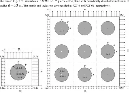
Example 2. A finite piezoelectric plane with a circular inclusion or periodically distributed inclusions (Fig. 3). In Fig. 3 (a), the dimension of the plane is

1.0 m 1.0 m

×

with a circular inclusion (radius

R

=

0.3 m

) at the center. Fig. 3 (b) describes a

3.0 m 3.0 m

×

piezoelectric plane with periodically distributed inclusions of radius

R

=

0.3 m

. The matrix and inclusions are specified as PZT-4 and PZT-6B, respectively.

(a) (b)

Fig. 3. A finite piezoelectric plane with (a) a circular inclusion; (b) periodically distributed

inclusions

For the

1.0 m 1.0 m

×

plane with one inclusion (see Fig. 3(a)), 10 nodes are distributed on each outer edge and 40 nodes on the inner boundary. The boundary conditions are

2

1 3 1

3 1 3

0.0 m,

0.0 Pa,

0.0 C/m

when 0.0 m

0.0 m,

0.0 Pa,

0.0 V

when 0.0 m

u

t

x

u

t

x

ω

φ

⎧ =

=

⎨

₌

⎩

and

2

1 3 1

2

3 1 3

0.001 m,

0.0 Pa,

0.0 C/m

when 1.0 m

0.001 m,

0.0 Pa,

0.0 C/m

when 1.0 m

u

t

x

u

t

x

ω

⎧ =

=

⎨

₌

⎩

Accordingly, for the

3.0 m 3.0 m

×

plane with periodically distributed inclusions (see Fig. 3(b)), 30 nodes are distributed on each outer edge and 40 nodes on each of the inner circular boundaries. The boundary conditions are

2

1 3 1

3 1 3

0.0 m,

0.0 Pa,

0.0 C/m

when 0.0 m

0.0 m,

0.0 Pa,

0.0 V

when 0.0 m

u

t

x

u

t

x

ω

φ

⎧ =

=

⎨

=

⎩

(10)

2

1 3 1

2

3 1 3

0.003 m,

0.0 Pa,

0.0 C/m

when 3.0 m

0.003 m,

0.0 Pa,

0.0 C/m

when 3.0 m

u

t

x

u

t

x

ω

⎧ =

=

⎨

₌

⎩

In Fig. 3 (a) and (b), three locations (labeled as point A, B, and C) on each of four representative inclusions (labeled as Inc 1 - Inc 4) are selected as reference points. At these points, the BNM results of displacement relative to their respective center of inclusion are given in Table 2 to verify the periodicity. Table 3 shows the comparison of the BNM results of electric potential at all reference points with the corresponding ones by ANSYS simulations.

Table 2

Comparison of results of BNM with the ones of ANSYS: displacement relative to the center of

inclusion.

ANSYS BNM Location

Inc 1 Inc 1 Inc 2 Inc 3 Inc 4

1

u

(m) 0.76947E−03 0.76950E−03 0.76945E−03 0.76945E−03 0.76951E−03

A 3

u

(m) 0.50005E−03 0.49987E−03 0.49982E−03 0.49982E−03 0.49987E−03

1

u

(m) 0.68906E−03 0.68904E−03 0.68889E−03 0.68889E−03 0.68904E−03

B 3

u

(m) 0.70594E−03 0.70596E−03 0.70599E−03 0.70599E−03 0.70595E−03

1

u

(m) 0.50000E−03 0.50000E−03 0.50000E−03 0.50000E−03 0.50000E−03

C 3

u

(m) 0.79148E−03 0.79148E−03 0.79182E−03 0.79182E−03 0.79148E−03

Table 3

Comparison of results of BNM with the ones of ANSYS: electric potential

φ

.

7

( 10 V)

φ

× on Inc 1

φ

( 10 V)× 7 on Inc 2

φ

( 10 V)× 7 on Inc 3

φ

( 10 V)× 7 on Inc 4 Locatio

n _{ANSYS BNM ANSYS} _{BNM ANSYS} _{BNM ANSYS BNM}

A 0.087222 0.087193 0.087206 0.087178 0.26162 0.26159 0.43605 0.43602

B 0.12149 0.12149 0.12151 0.12151 0.29592 0.29592 0.47031 0.47031

C 0.13560 0.13560 0.13583 0.13583 0.31024 0.31024 0.48443 0.48442

Based on the comparisons of this example, we note that the BNM scheme possesses encouraging accuracy when simulating this kind of piezoelectric composites.

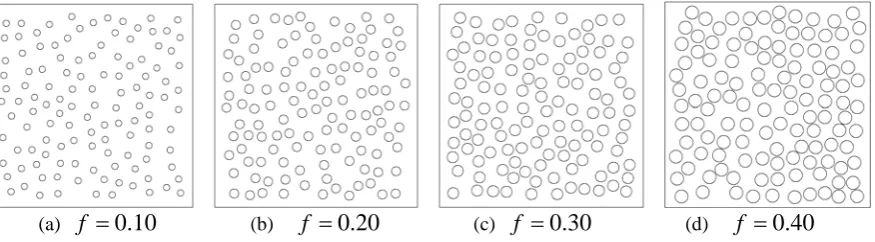
Example 3. Effective material constants of a finite piezoelectric plane with 120 randomly distributed inclusions (Fig. 4).

In this example, we calculate the effective material constants by implementing the models described in Section 6. The matrix and inclusions are specified as PZT-4 and PZT-6B, respectively. 100 nodes are distributed on each outer edge and 18 nodes on the inner boundary of each circular inclusion. The boundary conditions in Fig. 1 (a) - (c) are applied in this example to obtain the corresponding effective material constants.

(a)

f

=

0.10

(b)

f

=

0.20

(c)

f

=

0.30

(d)

f

=

0.40

(11)

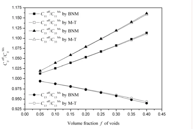
Figs. 5 and 6 display the normalized effective elastic, piezoelectric, and dielectric constants of PZT-4 ceramic as functions of inclusion volume fraction

f

. In this example, calculations of 8 cases of various volume fractions,

f

= 0.05, 0.10, 0.15, 0.20, 0.25, 0.30, 0.35, and 0.40 are performed. In these figures, the superscript “eff” indicates the effective material property and the superscript “Mx” indicates the material property of the matrix.

Fig. 5. Normalized effective elastic constants versus volume fraction of inclusions

Fig. 5 displays the normalized effective elastic constants versus volume fraction of inclusions. The numerical results by BNM are compared with the predictions by Mori-Tanaka model [24, 27]. This comparison tells that the numerical results of effective elastic constants agree very well with the analytical results by Mori-Tanaka at low volume fraction (say, lower than 0.25). Moreover, the differences between the numerical results and the analytical predictions increase with increasing volume fraction.

(12)

Fig. 6 shows the normalized effective piezoelectric constants

e

eff₃₁

/

e

Mx₃₁ ,

e

eff₃₃

/

e

Mx₃₃ and dielectric constant

eff Mx 33

/

33

κ

by BNM. They are also compared with the results by Mori-Tanaka model. These comparisons exhibit very well agreements between the numerical results and the analytical ones. It can be seen that the differences between the numerical results and the analytical predictions also increase with increasing volume fraction.

8. CONCLUSIONS

In this paper, a BNM scheme is presented to evaluate the effective properties of piezoelectric matrix with a large number of circular piezoelectric inclusions. The numerical results illustrate great agreement with the analytical predictions by Mori-Tanaka model. It shows that the BNM scheme is applicable to simulate structures of piezoelectric composites with inclusions of arbitrary distribution, since this scheme fully discretizes the outer boundaries and the inner matrix-inclusion interfaces of the entire physical domain. In this work, no assumptions are induced for discretizing the inner boundaries of inclusions, which means that this scheme can be easily extended to analyze the problems of piezoelectric materials with defects/inclusions of various shapes.

From the numerical examples and discussions, one can see that the BNM scheme inherits the virtue of high accuracy from BIE/BEM besides dimension reduction. It makes the BNM scheme be a promising approach to analyze the problems of composite materials with a large number of defects/inclusions of various shapes or structures with complex profile or configuration.

Acknowledgement The supports of the Special Foundation for the Authors of the Nationwide (China) Excellent Doctoral Dissertation (Project no: 200242) and the National Natural Science Foundation of China, under grant No. 10472051 are gratefully acknowledged.

REFERENCES

[1] Qin QH, Micromechanics-BE solution for properties of piezoelectric materials with defects, Engineering Analysis with Boundary Elements 2004; 28:809-814

[2] Day AR, Snyder KA, Garboczi EJ, Torpe MF, The elastic moduli of a sheet containing circular holes, Journal of the Mechanics and Physics of Solids 1992; 40:1031–1051.

[3] Jasius I, Chen C, Thorp MF, Elastic moduli of two-dimensional materials with polygonal and elliptical holes, Applied Mechanics Review 1994; 47:S18–S28.

[4] Kachanov M, Tsukrov I, Shafiro B, Eﬀective moduli of solids with cavities of various shapes, Applied Mechanics Review 1994; 47:S151–S174.

[5] Li ZH, Wang C, Chen CY, Effective electromechanical properties of transversely isotropic piezoelectric ceramics with microvoids, Computational Materials Science 2003; 27: 381-392

[6] Mori T, Tanaka K, Average stress in matrix and average elastic energy of materials with misfitting inclusions, Acta Metallica 1973; 21:571–574.

[7] Wu TL, Micromechanics determination of electroelastic properties of piezoelectric materials containing voids, Materials Science and Engineering A 2000; 280:320-327

[8] Qin QH, Yu SW. Effective moduli of thermopiezoelectric material with microcavities. Int J Solids Struct 1998; 35:5085–95.

[9] Qin QH. Fracture mechanics of piezoelectric materials. Southampton:WIT Press; 2000.

[10] Hu N, Wang B, Tan GW, Yao ZH, Yuan WF. Effective elastic properties of 2D solids with circular holes: numerical simulations. Compos Sci Technol 2000; 60:1811–23.

[11] Yao ZH, Kong FZ, Wang HT, Wang PB, 2D Simulation of composite materials using BEM, Engineering Analysis with Boundary Elements. 2004; 28:927–935

[12] KothnurVS, Mukherjee S, Mukherjee YX, Two-dimensional linear elasticity by the boundary node method, International Journal of Solids and Structures 1999; 36(8):1129-1147.

[13] Gu YT, Liu GR, A boundary point interpolation method for stress analysis of solids, Computational Mechanics 2002; 28:47-54.

[14] Zhang JM, Yao ZH, Tanaka M, The meshless regular hybrid boundary node method for 2D linear elasticity, Engineering Analysis with Boundary Elements 2003; 27(3):259-268.

[15] Lee JS, Boundary element method for electroelastic interaction in piezo ceramics, Engrg. Anal. Boundary Elements 1995; 15:321–328.

(13)

[17] Ding HJ, Chen WQ, Jiang AM, Green’s functions and boundary element method for transversely isotropic piezoelectric materials, Engineering Analysis with Boundary Elements 2004; 28:975-987

[18] Liu YJ, Fan H, On the conventional boundary integral equation formulation for piezoelectric solids with defects or of thin shapes, Engrg. Anal. Boundary Elements 2001; 25:77–91.

[19] Eshelby JD, The determination of the elastic field of an ellipsoidal inclusion and related problems, Proceedings of the Royal Society of London A 1957; 241:376–396.

[20] Sosa HA, Casto MA, Elastoelastric analysis of piezoelectric laminated structures, Appl. Mech. Rev. 1993; 46:21-28

[21] Sosa HA, Casto MA, On concentrated loads at the boundary of a piezoelectric half-plane, J. Mech. Phys. Solids 1994; 12: 1105-1122

[22] Dunn ML, Taya M, Micromechanics predictions of the eﬀective electroelastic moduli of piezoelectric composites, International Journal of Solids & Structures 1993; 30:161–175.

[23] Li JY, Dunn M, Variational bounds for the effective moduli of heterogeneous piezoelectric solids, Philosophical Magazine A. 2001; 81(4): 903-926

[24] Dunn M., Taya M., Electromechanical properties of porous piezoelectric ceramics, J. Am. Ceram. Soc.. 1993; 76(7):1697-1706

[25] Li JY, Dunn M, Analysis of microstructural fields in heterogeneous piezoelectric solids, Int. J. of Engng. Sci., 1999; 37: 665-685.

[26] Mukherjee YX, Mukherjee S., The boundary node method for potential problems, International Journal for Numerical Methods in Engineering. 1997; 40:797-815.

[27] Mikata Y, Determination of piezoelectric Eshelby tensor in transversely isotropic piezoelectric solids, International Journal of Engineering Science. 2000; 38:605-641.

Applications of Boundary Node Method to Simulation of Piezoelectric Composites