J
INGNI
L
I
,
R
ADA
C
HIRKOVA
,
AND
Y
AHYA
F
ATHI
A
N
IP
M
ODEL FOR THE
V
IEW
S
ELECTION
P
ROBLEM
(Technical Report)
December 7, 2004
Abstract:
A commonly used and powerful technique for improving query response time over large databases is to materialize frequently asked queries. The problem is to select an appropriate set of views, given a limited amount of storage resources. The
contribution of this project is the integer programming model that is developed to solve the view selection problem. Given a list of queries and a lattice, return the definition of the materialized views. Moreover, the view selection problem can be compared with the UFL and k-Median problem that are well defined and analyzed in IP area.
Abstract: ... 2
1. Introduction... 4
2. Integer Programming model ... 4
2.1 Parameters and Variables... 4
2.2 Integer Programming Model... 5
2.3 Example ... 6
3. Data Structure ... 7
4. Experiments by exact method ... 8
4.1 Solve three instances of different workload... 8
4.2 Sensitivity Analysis on b ... 9
4.3 Variation in the query list ... 13
5. LP relaxation and Lower Bound ... 16
6. The Greedy Algorithm... 19
6.1 Algorithm outline ... 20
6.2 Solve the three instances by greedy algorithm... 20
7. Comparison with UFL and k-Median problem... 21
8. Conclusion ... 24
References ... 25
Appendix ... 26
1. AMPL file for the small example... 26
2. AMPL model file... 27
3. Matlab file to generate AMPL data file ... 28
1. Introduction
Decision support system involves complex queries on large databases. A common and powerful query optimization technique is to materialize some queries instead of computing them from raw data each time. But we can not materialize all the queries when the storage space is limited. Thus it is critical to select an appropriate set of views to materialize to improve the performance of frequent and important queries. The dependency among the views is defined by the lattice. Suppose a list of queries and a lattice in database are already given, the goal of the project is to develop an efficient integer programming model for the view select problem in the case that each query can be answered by one qualified view in the lattice framework.
The project report is organized as follows. In Section 2, we introduce the IP model to represent the view selection problem in mathematical way. In Section 3, we present the data structure for each node of view in the lattice. In Section 4, we solve several instances of the IP with quite different sizes by mathematical programming software package AMPL/CPLEX and do the sensitivity analysis experiments on the value of b. In Section 5, we compute the lower bound for the IP problem by solving its LP relaxation. In Section 6, we implement the greedy algorithm to the view selection problem and compare the result with those got from exact method. Section 7 compares the view selection problem with UFL and k-Median problems in IP that have been well developed. Finally, Section 8 summarizes the results in this project and plans some further work in the future.
2. Integer Programming model
In this project report, we skip the work about how to generate the lattice but
concentrate on the optimization part. Given the tables in the large relational database, a lattice framework can be constructed to express dependencies among views. A query can be answered by any one of its ancestors in the lattice that includes the raw data and itself. Assume that the lattice based on the database and the set of queries to be answered are already given. The objective is to materialize a subset of right views in the lattice to minimize the time cost to answer the required queries subject to the storage space constraints. The materialized views must be precomputed and stored on disk, and the storage space of a view is set to be linear to the number of rows in the view. The time to answer a query is taken to be equal to the storage space occupied by the view from which the query is answered.
There are n views in the lattice and m queries to be answered. The input is the cost vector associated with each view, the queries to be answered and the storage space limit, while the output is the views that need to be materialized.
2.1 Parameters and Variables
Declare the parameters of this IP:
j: Index of queries j = 1 to m
Let ai be the number of rows in viewi.
Let b be the storage space limit.
Let cij be the cost to answer query j by using viewi.
if view i can used to answer query j otherwise i
ij
a
c =
∞
Define the variables of this IP:
Let 1 if view i is materialized 0 otherwise
i x
=
Let 1 if we use view i to answer query j 0 otherwise
ij y
=
2.2 Integer Programming Model
Formulate the IP model: Mininmize
,
ij ij i j
c y
∀
Subject to:
1
n
i i i
a x b
=
≤
1 1 n
ij i
y j
= = ∀
, where
ij i ij
y ≤x ∀i j c ≠Inf
1 1 x =
= 0 or 1 0 ,
i
ij
x i
y i j
∀ ≥ ∀
The first constraint is the storage constraint which limits the total number of rows in the materialized views to be no more than the current storage space. The second set of constraints guarantee that each query must be answered by any one view in the lattice. The third set of constraints shows that no query can be answered be view j if view j is not materialized. For each i, considering only those views that can be used to answer query j, wherecij≠Inf , decreases the number of constraints. The fourth constraint
2.3 Example
In this part, we show a small example to verify our IP model.
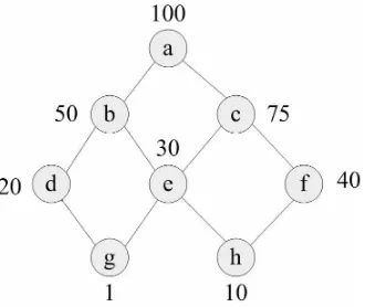
Given the lattice of Example 4.1 in Page 13 of Ullman’s paper in the following Figure 1,
Figure 1: Example lattice with space costs We can get the cost matrix as follows.
[
100 50 75 20 30 40 1 10]
ta=
100 100 100 100 100 100 100 100
50 50 50 50 50
75 75 75 75 75
20 20
30 30 30
40 40
1 10
c
∞ ∞ ∞
∞ ∞ ∞
∞ ∞ ∞ ∞ ∞ ∞
=
∞ ∞ ∞ ∞ ∞
∞ ∞ ∞ ∞ ∞ ∞
∞ ∞ ∞ ∞ ∞ ∞ ∞
∞ ∞ ∞ ∞ ∞ ∞ ∞
Solve the IP problem using AMPL/CPLEX and get the same solution as that in that paper. The solution indicates that in order to attain the minimal cost to answer all the 8 queries, we should materialize view 2, 4, 6 (corresponding to b, d, f in the lattice graph) besides the raw data and thus achieve the optimal cost of 420. The code file for this example is attached to the end of the report.
3. Data Structure
In this section, we analyze the data set file that comes from the real world. The data about the lattice that comes from the realistic world contains two columns. Each row in the data file that corresponds to a node in the lattice has a view ID and a view size. The view size here is taken to be the number of rows in the view. Given the workload of the number of attributes, the structure of the lattice and dependency among the views are fixed. The only variation is the view size associated with each node in the lattice. We define the data structure of each node, which can be used to express the relationship among the views and can be tracked back to the definition of the derived views once we get the solution of the IP model.
Suppose the workload of the attributes from the database is K. The number of nodes in the lattice is 2Kand it increases exponentially as the number of attributes increases. For each node in the lattice, let the binary vector define the characteristics whether or not each attributes is used to aggregate the tuples in database. It is equal to 1 if the attribute has the characteristics at this node and 0 otherwise. Then each node can be express by a 0-1 vector and the dependency can be derived expressively from this kind of data structure. A view in the lattice can be computed directly from its ancestor if there is dependency relationship between them. In the example shown in Table 1, we compare each element in any pair of vector E and F. If there exists any element that is equal to 1 in E while the corresponding element in F is 0, then view F can not be used to answer view E as shown.
Table 1. Dependency expressed by binary vector View View ID View Definition
E 5 1, 0, 1
F 4 1, 0, 0
4. Experiments by exact method
In realistic world, the total space available to store the materialized views is usually smaller than the cost of the objective queries. Otherwise we can precompute all the queries in advance and store them on disk, and then there is no need to optimize this view selection problem. Moreover, the available storage space is no more than five times than the raw data because we would rather not spend that much to store those materialized. There is a tradeoff between the cost and the efficiency during the decision process.
4.1 Solve three instances of different workload.
Given the lattice, we can get the input for the IP model in section 2. The structure of the parameters and variables for the three instances is shown as follows in Table 2. The cardinality of vector A is smaller than the number of nodes in the lattice because we skip those nodes that can not be used to answer anyone in the query list and those views have been taken to be zero in the dataset file. Then the number of rows in the cost matrix C is taken to be the same as that in A and the number of columns in C is equal to the cardinality of the query set. We use Matlab to write the input data file for the IP model and then use AMPL/CPLEX to solve the IP instances. The timing of each workload instance is shown in the following Table 3, in the unit of the system CPU seconds.
Table 2. Sizes of the problem
Workload Number of nodes Number of queries A C X Y
View_7 128 7 60×1 60×7 60×1 60×7
View_13 8192 8 4104×1 4104×8 4104×1 4104×8
View_15 32768 8 17464×1 17464×8 17464×1 17464×8
Table 3. Timing of Matlab and AMPL/CPLEX Workload Matlab AMPL/CPLEX Total Time View_7 0.22s 0.05s 0.27s View_13 20.91s 3.04s 23.95s View_15 391.20s 18.64s 409.84s
Given three realistic instances of different workload size which is 7, 13 and 15, we can solve them by AMPL/CPLEX by setting a reasonable storage space limit b. Let R denote the number of rows in the raw data.
Let W denote the total number of rows in the queries in the objective list. Setb=min
{
R+β θW, R}
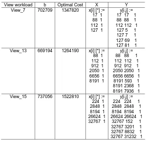
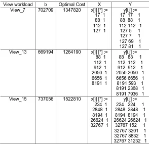
, where0≤ ≤β 1,θ >1.Table 4. Results of solving three instances
View workload b Optimal Cost X Y
View_7 702709 1347820 x[i] [*] := 17 1 88 1 112 1 127 1
y[i,j] := 17 17 1 88 88 1 112 112 1
127 5 1 127 7 1 127 69 1 127 81 1 View_13 669194 1264190 x[i] [*] :=
88 1 112 1 912 1 2050 1 6656 1 8191 1
y[i,j] := 88 88 1 112 112 1 912 912 1 2050 2050 1 6656 6656 1 8191 593 1 8191 2368 1 8191 7936 1 View_15 737056 1522810 x[i] [*] :=
224 1 2848 1 8194 1 26624 1 32767 1
y[i,j] := 224 224 1 2848 2848 1 8194 8194 1 26624 26624 1
32767 152 1 32767 3201 1 32767 8832 1 32767 31232 1
4.2 Sensitivity Analysis on b
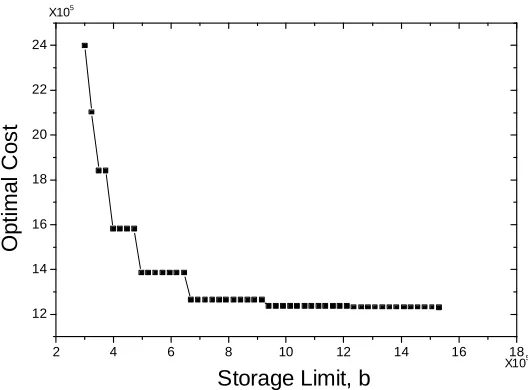
Intuitively, the optimal cost decreases as the storage space increases. If we have limited space that can only store the raw data, then every query must compute directly from the root node and the evaluation cost to answer all the queries is the number of the queries times the cost of the raw data. If we have space to store all the queries precomputed, there is no optimization issues in this case and the total evaluation cost is simply the summation of the cost of all the queries.
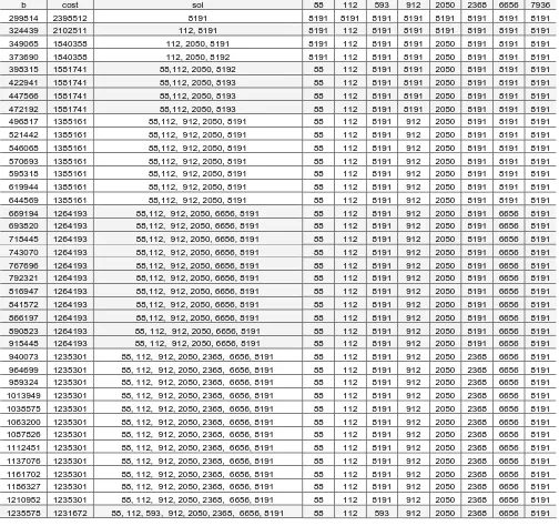
In Table 4 as follows, we do the sensitivity analysis on b for the view-7 and view-13 workload instances. Given the same query list as in section 4.1, as the storage space limit increases in the above range, the optimal cost decreases step piece wise. Unless there is more space available that is large enough to hold one more materialized query, the evaluation cost remains the same for the given objective query list. As shown in Table 5 and 6, the first column b is the storage space limit. The first value b takes is the number of rows in the raw data and the last value it takes is the cost of the raw data plus the total cost of the queries. Since the query list is short in the given instances, the total cost of the queries never exceeds the threshold of five times the raw data. The second column is the optimal objective value of the IP model for the given b. The third column corresponds to X in the model which is the optimal
piece wise as the value of b increases. Within the range in each piece, the objective value and the optimal solution remain the same. They only change when the value of b grows big enough to hold another possible materialized view.
Table 5. Sensitivity analysis results on b for view-7 instance
b cost sol 5 7 17 69 81 88 112
299814 2098698 127 127 127 127 127 127 127 127
326674 1802697 112,127 127 127 127 127 127 127 112
353533 1544080 88,112,127 127 127 127 127 127 88 112
380393 1544080 88,112,127 127 127 127 127 127 88 112
407253 1544080 112,120,127 127 127 127 127 127 120 112
434113 1544080 112,120,127 127 127 127 127 127 120 112
460972 1347815 17,88,112,127 127 127 17 127 127 88 112
487832 1347815 17,88,112,127 127 127 17 127 127 88 112
514692 1347815 17,88,112,127 127 127 17 127 127 88 112
541551 1347815 17,88,112,127 127 127 17 127 127 88 112
568411 1347815 17,88,112,127 127 127 17 127 127 88 112
595271 1347815 17,88,112,127 127 127 17 127 127 88 112
622131 1347815 17,88,112,127 127 127 17 127 127 88 112
648990 1347815 17,88,112,127 127 127 17 127 127 88 112
675850 1347815 17,88,112,127 127 127 17 127 127 88 112
702710 1347815 17,88,112,127 127 127 17 127 127 88 112
729570 1347815 17,88,112,127 127 127 17 127 127 88 112
756429 1344186 17,81,88,112,127 127 127 17 127 81 88 112
783289 1344186 17,81,88,112,127 127 127 17 127 81 88 112
810149 1344186 17,81,88,112,127 127 127 17 127 81 88 112
837008 1344186 17,81,88,112,127 127 127 17 127 81 88 112
863868 1344186 17,81,88,112,127 127 127 17 127 81 88 112
890728 1344186 17,81,88,112,127 127 127 17 127 81 88 112
917588 1344186 17,81,88,112,127 127 127 17 127 81 88 112
944447 1344186 17,81,88,112,127 127 127 17 127 81 88 112
971307 1344186 17,81,88,112,127 127 127 17 127 81 88 112
998167 1344186 17,81,88,112,127 127 127 17 127 81 88 112
1025026 1344186 17,81,88,112,127 127 127 17 127 81 88 112
1051886 1343013 5,17,81,88,112,127 5 127 17 127 81 88 112
1078746 1343013 5,17,81,88,112,127 5 127 17 127 81 88 112
1105606 1343013 5,17,81,88,112,127 5 127 17 127 81 88 112
1132465 1343013 5,17,81,88,112,127 5 127 17 127 81 88 112
1159325 1343013 5,17,81,88,112,127 5 127 17 127 81 88 112
1186185 1343013 5,17,81,88,112,127 5 127 17 127 81 88 112
1213044 1343013 5,17,81,88,112,127 5 127 17 127 81 88 112
1239904 1343013 5,17,81,88,112,127 5 127 17 127 81 88 112
1266764 1343013 5,17,81,88,112,127 5 127 17 127 81 88 112
1293624 1343013 5,17,81,88,112,127 5 127 17 127 81 88 112
1320483 1343013 5,17,81,88,112,127 5 127 17 127 81 88 112
1347343 1342994 5,7,17,81,88,112,127 5 7 17 127 81 88 112
1374203 1342994 5,7,17,81,88,112,127 5 7 17 127 81 88 112
1427922 1342994 5,7,17,81,88,112,127 5 7 17 127 81 88 112
1454782 1342994 5,7,17,81,88,112,127 5 7 17 127 81 88 112
1481642 1342994 5,7,17,81,88,112,127 5 7 17 127 81 88 112
1508501 1342994 5,7,17,81,88,112,127 5 7 17 127 81 88 112
1535361 1342994 5,7,17,81,88,112,127 5 7 17 127 81 88 112
1562221 1342994 5,7,17,81,88,112,127 5 7 17 127 81 88 112
1589081 1342994 5,7,17,81,88,112,127 5 7 17 127 81 88 112
1615940 1342994 5,7,17,81,88,112,127 5 7 17 127 81 88 112
1642800 1342986 5,7,17,69,81,88,112,127 5 7 17 69 81 88 112
Table 6. Sensitivity analysis results on b for view-13 instance
b cost sol 88 112 593 912 2050 2368 6656 7936
299814 2398512 8191 8191 8191 8191 8191 8191 8191 8191 8191
324439 2102511 112, 8191 8191 112 8191 8191 8191 8191 8191 8191
349065 1840358 112, 2050, 8191 8191 112 8191 8191 2050 8191 8191 8191
373690 1840358 112, 2050, 8192 8191 112 8191 8191 2050 8191 8191 8191
398315 1581741 88,112, 2050, 8192 88 112 8191 8191 2050 8191 8191 8191
422941 1581741 88,112, 2050, 8193 88 112 8191 8191 2050 8191 8191 8191
447566 1581741 88,112, 2050, 8193 88 112 8191 8191 2050 8191 8191 8191
472192 1581741 88,112, 2050, 8193 88 112 8191 8191 2050 8191 8191 8191
496817 1385161 88,112, 912, 2050, 8191 88 112 8191 912 2050 8191 8191 8191
521442 1385161 88,112, 912, 2050, 8191 88 112 8191 912 2050 8191 8191 8191
546068 1385161 88,112, 912, 2050, 8191 88 112 8191 912 2050 8191 8191 8191
570693 1385161 88,112, 912, 2050, 8191 88 112 8191 912 2050 8191 8191 8191
595318 1385161 88,112, 912, 2050, 8191 88 112 8191 912 2050 8191 8191 8191
619944 1385161 88,112, 912, 2050, 8191 88 112 8191 912 2050 8191 8191 8191
644569 1385161 88,112, 912, 2050, 8191 88 112 8191 912 2050 8191 8191 8191
669194 1264193 88,112, 912, 2050, 6656, 8191 88 112 8191 912 2050 8191 6656 8191
693820 1264193 88,112, 912, 2050, 6656, 8191 88 112 8191 912 2050 8191 6656 8191
718445 1264193 88,112, 912, 2050, 6656, 8191 88 112 8191 912 2050 8191 6656 8191
743070 1264193 88,112, 912, 2050, 6656, 8191 88 112 8191 912 2050 8191 6656 8191
767696 1264193 88,112, 912, 2050, 6656, 8191 88 112 8191 912 2050 8191 6656 8191
792321 1264193 88,112, 912, 2050, 6656, 8191 88 112 8191 912 2050 8191 6656 8191
816947 1264193 88,112, 912, 2050, 6656, 8191 88 112 8191 912 2050 8191 6656 8191
841572 1264193 88,112, 912, 2050, 6656, 8191 88 112 8191 912 2050 8191 6656 8191
866197 1264193 88,112, 912, 2050, 6656, 8191 88 112 8191 912 2050 8191 6656 8191
890823 1264193 88, 112, 912, 2050, 6656, 8191 88 112 8191 912 2050 8191 6656 8191
915448 1264193 88, 112, 912, 2050, 6656, 8191 88 112 8191 912 2050 8191 6656 8191
940073 1235301 88, 112, 912, 2050, 2368, 6656, 8191 88 112 8191 912 2050 2368 6656 8191
964699 1235301 88, 112, 912, 2050, 2368, 6656, 8191 88 112 8191 912 2050 2368 6656 8191
989324 1235301 88, 112, 912, 2050, 2368, 6656, 8191 88 112 8191 912 2050 2368 6656 8191
1013949 1235301 88, 112, 912, 2050, 2368, 6656, 8191 88 112 8191 912 2050 2368 6656 8191
1038575 1235301 88, 112, 912, 2050, 2368, 6656, 8191 88 112 8191 912 2050 2368 6656 8191
1063200 1235301 88, 112, 912, 2050, 2368, 6656, 8191 88 112 8191 912 2050 2368 6656 8191
1087826 1235301 88, 112, 912, 2050, 2368, 6656, 8191 88 112 8191 912 2050 2368 6656 8191
1112451 1235301 88, 112, 912, 2050, 2368, 6656, 8191 88 112 8191 912 2050 2368 6656 8191
1137076 1235301 88, 112, 912, 2050, 2368, 6656, 8191 88 112 8191 912 2050 2368 6656 8191
1161702 1235301 88, 112, 912, 2050, 2368, 6656, 8191 88 112 8191 912 2050 2368 6656 8191
1186327 1235301 88, 112, 912, 2050, 2368, 6656, 8191 88 112 8191 912 2050 2368 6656 8191
1210952 1235301 88, 112, 912, 2050, 2368, 6656, 8191 88 112 8191 912 2050 2368 6656 8191
1260203 1231672 88, 112, 593, 912, 2050, 2368, 6656, 8191 88 112 593 912 2050 2368 6656 8191
1284828 1231672 88, 112, 593, 912, 2050, 2368, 6656, 8191 88 112 593 912 2050 2368 6656 8191
1309454 1231672 88, 112, 593, 912, 2050, 2368, 6656, 8191 88 112 593 912 2050 2368 6656 8191
1334079 1231672 88, 112, 593, 912, 2050, 2368, 6656, 8191 88 112 593 912 2050 2368 6656 8191
1358704 1231672 88, 112, 593, 912, 2050, 2368, 6656, 8191 88 112 593 912 2050 2368 6656 8191
1383330 1231672 88, 112, 593, 912, 2050, 2368, 6656, 8191 88 112 593 912 2050 2368 6656 8191
1407955 1231672 88, 112, 593, 912, 2050, 2368, 6656, 8191 88 112 593 912 2050 2368 6656 8191
1432581 1231672 88, 112, 593, 912, 2050, 2368, 6656, 8191 88 112 593 912 2050 2368 6656 8191
1457206 1231672 88, 112, 593, 912, 2050, 2368, 6656, 8191 88 112 593 912 2050 2368 6656 8191
1481831 1231672 88, 112, 593, 912, 2050, 2368, 6656, 8191 88 112 593 912 2050 2368 6656 8191
1506457 1231672 88, 112, 593, 912, 2050, 2368, 6656, 8191 88 112 593 912 2050 2368 6656 8191
1531082 1231268 88, 112, 593, 912, 2050, 2368, 6656, 7936, 8191 88 112 593 912 2050 2368 6656 7936
2 4 6 8 10 12 14 16 18
13 14 15 16 17 18 19 20 21 22X10
5
X105
O
p
ti
m
a
l
C
o
s
t
Storage Limit, b
Figure 2. Sensitivity analysis on b for view-7 instance
2 4 6 8 10 12 14 16 18
12 14 16 18 20 22 24
X105
X105
O
p
ti
m
a
l
C
o
s
t
Storage Limit, b
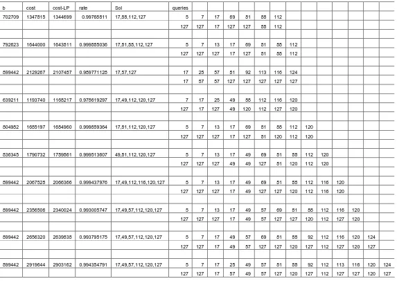
4.3 Variation in the query list
Table 7. Variation in the query list for view_7 instance
b cost cost-LP rate Sol queries
702709 1347815 1344699 0.99768811 17,88,112,127 5 7 17 69 81 88 112
127 127 17 127 127 88 112
792623 1644000 1643811 0.999885036 17,81,88,112,127 5 7 13 17 69 81 88 112
127 127 127 17 127 81 88 112
899442 2129267 2107487 0.989771128 17,57,127 17 25 57 81 92 113 116 124
17 57 57 127 127 127 127 127
639211 1193740 1168217 0.978619297 17,49,112,120,127 7 17 25 49 88 112 116 120
127 17 127 49 120 112 127 120
804982 1685197 1684960 0.999859364 17,81,112,120,127 5 7 13 17 69 81 88 112 120
127 127 127 17 127 81 120 112 120
836345 1790732 1789861 0.999513607 49,81,112,120,127 5 7 13 17 49 69 81 88 112 120
127 127 127 49 49 127 81 120 112 120
899442 2067528 2066366 0.999437976 17,49,112,116,120,127 5 7 13 17 49 69 81 88 112 116 120
127 127 127 17 49 127 127 120 112 116 120
899442 2356506 2340024 0.993005747 17,49,57,112,120,127 5 7 13 17 49 57 69 81 88 112 116 120
127 127 127 17 49 57 127 127 120 112 127 120
899442 2656320 2639838 0.993795175 17,49,57,112,120,127 5 7 17 49 57 69 81 88 92 112 116 120 124
127 127 17 49 57 127 127 120 127 112 127 120 127
899442 2919644 2903162 0.994354791 17,49,57,112,120,127 5 7 17 25 49 57 81 88 92 112 113 116 120 124
Table 8. Variation in the query list for view_13 instance
b cost cost-LP rate Sol Queries
669194 1264193 1263699 0.999609237 88, 112, 912, 2050, 6656, 8191 88 112 593 912 2050 2368 6656 7936
88 112 8191 912 2050 8191 6656 8191
481648 836777 800684 0.956866644 88, 3078, 3110, 4208, 8191 88 112 368 2050 3078 3110 4208 7936
88 4208 8191 3078 3078 3110 4208 8191
494007 862847 811646 0.940660395 112, 120, 3078, 3110, 4208, 8191 88 112 120 368 2050 3078 3110 4208 7936
120 112 120 8191 3078 3078 3110 4208 8191
481759 1232346 1205459 0.978182264 120, 3074, 3110, 4208, 8191 88 120 368 945 2050 2082 2160 3074 3110 4208
120 120 8191 8191 3074 3110 8191 3074 3110 4208
501997 1192077 1172008 0.983164678 120, 3106, 4464, 8191 88 112 120 368 945 2050 2082 2160 3074 3106 4464
120 120 120 4464 8191 3106 3106 8191 3106 3106 4464
592514 1384708 1267478 0.915339552 112, 120, 2054, 3074, 3106, 4464, 8191 88 112 120 368 945 2054 2082 2160 3106 4464 7936
120 112 120 4464 8191 2054 3106 8191 3106 4464 8191
668998 1473472 1404291 0.953048989 112, 120, 2160, 3078, 3106, 4464, 8191 88 112 120 344 368 945 2054 2082 2160 3074 4464 7936
120 112 120 8191 4464 8191 3078 3106 2160 3078 4464 8191
731857 1663128 1586692 0.954040819 112, 120, 2160, 3110, 4464, 5041, 8191 88 112 120 344 368 624 945 2054 2082 2160 3074 3106 4464 7936
120 112 120 8191 4464 8191 5041 3110 3110 2160 3110 3110 4464 8191
554554 1334638 1284152 0.962172514 112, 120, 3074, 3110, 4464, 8191 88 112 120 368 945 2050 2082 2086 2160 3074 3106 3110 4208 4464
120 112 120 4464 8191 3074 3110 3110 8191 3074 3110 3110 4464 4464
547176 1156782 1129862 0.976728545 120, 3078, 3110, 4464, 8191 88 112 120 368 2050 2054 2082 2086 2160 3074 3078 3106 3110 4208 4464
5. LP relaxation and Lower Bound
The linear programming relaxation can give a lower bound of the IP problem. If solving the LP relaxation gives integer solution, the IP problem can be simple solved by its LP version. Otherwise, the result of objective value of the LP defines a lower bound for the IP problem and it can be derived that the optimal value of the IP is no smaller than that of the LP problem.
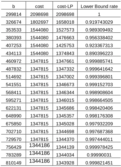
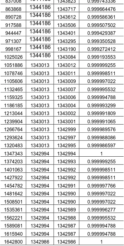
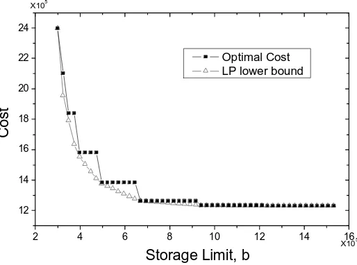
In Table 9 and 10, we get the lower bound given by the LP relaxation for the same range of b in section 4.2. As we can see in the following tables, the LP lower bound is very close to the optimal value of the IP problem most of the time. We also compare the LP lower bound with the optimum in Table 7 and 8 when we do the sensitivity analysis for the variations on the queries. Linear programming relaxation provides good lower bound in all the instances and the ratio of the lower bound to the optimum is ninety-nine percent for most of the cases. The distance between the LP lower bound and the optimal value varies as the value of b changes. Because in the LP problem, X can take any value between 0 and 1, and then the knapsack constraint, which is the first constraint of the storage limit in the model, is always binding. While in the IP problem, X is binary variables and the knapsack constraint is not active sometime and there is some space left that is not big enough to hold one more useful materialized view. Thus the optimal value of the LP problem is continuous while the optimal value of the IP problem is step piece wise as b changes within the range.
Table 9. Sensitivity Analysis and LP Lower Bound for view_7 instances
b cost cost-LP Lower Bound rate
299814 2098698 2098698 1
326674 1802697 1658018 0.919743029
353533 1544080 1527573 0.989309492
380393 1544080 1476663 0.956338402
407253 1544080 1425753 0.923367313
434113 1544080 1374843 0.890396223
460972 1347815 1347661 0.999885741
487832 1347815 1347332 0.999641642
514692 1347815 1347002 0.999396801
541551 1347815 1346673 0.999152703
568411 1347815 1346344 0.998908604
595271 1347815 1346015 0.998664505
622131 1347815 1345686 0.998420406
648990 1347815 1345357 0.998176308
675850 1347815 1345028 0.997932209
702710 1347815 1344698 0.997687368
729570 1347815 1344370 0.997444011
756429 1344186 1344139 0.999978425
783289 1344186 1344034 0.99990031
837008 1344186 1343823 0.999743336
863868 1344186 1343717 0.999664476
890728 1344186 1343612 0.999586361
917588 1344186 1343506 0.999507502
944447 1344186 1343401 0.999429387
971307 1344186 1343295 0.999350528
998167 1344186 1343190 0.999272412
1025026 1344186 1343084 0.999193553
1051886 1343013 1343012 0.999999255
1078746 1343013 1343011 0.999998511
1105606 1343013 1343009 0.999997022
1132465 1343013 1343007 0.999995532
1159325 1343013 1343006 0.999994788
1186185 1343013 1343004 0.999993299
1213044 1343013 1343002 0.999991809
1239904 1343013 1343001 0.999991065
1266764 1343013 1342999 0.999989576
1293624 1343013 1342997 0.999988086
1320483 1343013 1342995 0.999986597
1347343 1342994 1342994 1
1374203 1342994 1342993 0.999999255
1401063 1342994 1342992 0.999998511
1427922 1342994 1342992 0.999998511
1454782 1342994 1342991 0.999997766
1481642 1342994 1342990 0.999997022
1508501 1342994 1342990 0.999997022
1535361 1342994 1342989 0.999996277
1562221 1342994 1342988 0.999995532
1589081 1342994 1342987 0.999994788
1615940 1342994 1342987 0.999994788
1642800 1342986 1342986 1
Table 10. Sensitivity Analysis and LP Lower Bound for view_13 instances
b cost cost-LP Lower Bound rate
299814 2398512 2398512 1
324439 2102511 1957642 0.93109715
349065 1840358 1791537 0.973472009
373690 1840358 1636952 0.889474765
398315 1581741 1551597 0.980942518
422941 1581741 1504704 0.951296072
447566 1581741 1457813 0.92165089
472192 1581741 1410919 0.892003811
496817 1385161 1377655 0.994581135
521442 1385161 1360999 0.98255654
546068 1385161 1344329 0.970521838
570693 1385161 1327686 0.958506628
595318 1385161 1311030 0.946482033
644569 1385161 1277718 0.922432844
669194 1264193 1263699 0.999609237
693820 1264193 1261073 0.997532022
718445 1264193 1258447 0.995454808
743070 1264193 1255821 0.993377593
767696 1264193 1253195 0.991300379
792321 1264193 1250568 0.989222373
816947 1264193 1247942 0.987145159
841572 1264193 1245316 0.985067945
866197 1264193 1242690 0.98299073
890823 1264193 1240064 0.980913516
915448 1264193 1237438 0.978836301
940073 1235301 1235245 0.999954667
964699 1235301 1234943 0.999710192
989324 1235301 1234641 0.999465717
1013949 1235301 1234340 0.999222052
1038575 1235301 1234038 0.998977577
1063200 1235301 1233736 0.998733102
1087826 1235301 1233434 0.998488627
1112451 1235301 1233133 0.998244962
1137076 1235301 1232831 0.998000487
1161702 1235301 1232529 0.997756013
1186327 1235301 1232228 0.997512347
1210952 1235301 1231926 0.997267872
1235578 1231672 1231667 0.99999594
1260203 1231672 1231633 0.999968336
1284828 1231672 1231600 0.999941543
1309454 1231672 1231567 0.99991475
1334079 1231672 1231534 0.999887957
1358704 1231672 1231501 0.999861164
1383330 1231672 1231467 0.99983356
1407955 1231672 1231434 0.999806767
1432581 1231672 1231401 0.999779974
1457206 1231672 1231368 0.999753181
1481831 1231672 1231334 0.999725576
1506457 1231672 1231301 0.999698783
2 4 6 8 10 12 14 16 13
14 15 16 17 18 19 20 21 22
Optimal Cost LP lower bound
X105
X105
C
o
s
t
Storage Limit, b
Figure 4. Sensitivity analysis and LP lower bound for view-7 instance
2 4 6 8 10 12 14 16
12 14 16 18 20 22 24
Optimal Cost LP lower bound
X105
X105
C
o
s
t
Storage Limit, b
Figure 5. Sensitivity analysis and LP lower bound for view-13 instance
6. The Greedy Algorithm
6.1 Algorithm outline
Let A(v) be the cost of view i. Let Q be the objective queries to be answered. Given a set of materialized views S, let S denote the complementary view selection space.
Let C(S) be the cost to answer Q by utilizing the materialized views in S. Suppose also that there is a limit b on the storage space, including the raw data, let b(S) be the space left after set S is stored. Let B(v, S) the benefit of view v relative to S after selecting some set S of views including the top view. B(v, S) is computed as the difference between C({v, S}) and C(S). At each step of the iteration, the view v* that can maximize the positive benefit in the current step is selected if A(v*) is no more than the remaining storage space. Let D be the search space of all qualified views. Observe that for a given set of objective queries, the number of materialized views is no more than the number of objective queries since each query is to be answered by any one view in the lattice.
The iteration stops where there is no enough available space to hold any one more view or the number of selected materialized view reaches the number of queries. Now, we can define the Greedy Algorithm for the view-selection problem as follows. Step 0: Initialization.
S = {raw data}; Step 1: Stopping.
If
{
( )
}
( )
v S
Min A v b S
∈ ≤ and S < Q , go to step 2. Otherwise, stop.
Step 2: Local Optimization. Choose view v such that
( )
( )
( )
, 0 ( ), arg
v S A v b S
B v S
v Max
A v
∈ < <
=
where B v S
( )
, >0. Then update{ }
v S, →S and go to step 1.6.2 Solve the three instances by greedy algorithm
Using the above greedy algorithm and code it into Matlab function , we can solve the three instances with the same parameter and variable definition in section 4.1.
Setb=min
{
R+β θW, R}
, where0≤ ≤β 1,θ >1.We solve the three instances forβ =.3,θ =3 in Table 11 by greedy algorithm
View workload b Optimal Cost X Y View_7 702709 1347820 x[i] [*] :=
17 1 88 1 112 1 127 1
y[i,j] := 17 17 1 88 88 1 112 112 1
127 5 1 127 7 1 127 69 1 127 81 1 View_13 669194 1264190 x[i] [*] :=
88 1 112 1 912 1 2050 1 6656 1 8191 1
y[i,j] := 88 88 1 112 112 1 912 912 1 2050 2050 1 6656 6656 1 8191 593 1 8191 2368 1 8191 7936 1 View_15 737056 1522810 x[i] [*] :=
224 1 2848 1 8194 1 26624 1 32767 1
y[i,j] := 224 224 1 2848 2848 1 8194 8194 1 26624 26624 1
32767 152 1 32767 3201 1 32767 8832 1 32767 31232 1
Although the greedy algorithm gives the same results in the three instances as we get by exact method solved by AMPL/CPLEX in section 4.1, there is no guarantee that it is always the case. For a counterexample as shown in Table 12, We solve the view_7 instance for other value of b and find that the result given by the greedy algorithm is not optimal. The ratio may depend on several factors including the lattice structure, the query list and the value of b. We leave this direction of research for future work.
Table 12. Non-optimal results of view_7 instance by greedy algorithm (GA) View workload b Optimal Cost Cost given by GA X(optimal) X(GA)
View_7 971307 1344186 1346642 x[i] [*] := 17 1 81 1 88 1 112 1 127 1
x[i] [*] := 5 1 17 1 88 1 112 1 127 1
7. Comparison with UFL and k-Median problem
As we know, Uncapacited Facility Location problem (UFL) and k-Median problem have been well developed in IP research area and there are a lot of efficient
algorithms related to these two problems. We review some basic idea about these two problems as follows.
Given:
n Potential facility locations
m Clients
j
f Fixed cost of opening a facility at location j
ij
c Cost of serving client i from facility j
j
y Binary variable designating whether facility j is open
ij
x Binary variable designating whether client i is assigned to facility j The IP model for UFL problem is as follows.
Minimize
1 1 1
n m n
j j ij ij
j i j
z f y c x
= = =
= +
Subject to
1
1
,
, =0 or 1 ,
n ij j
ij j ij j
x i
x y i j x y i j
= = ∀
≤ ∀
∀
The objective is to select a set of facility locations and assign each client to a facility to minimize total cost. The first set of constraints defines that every client must be assigned to some facility to satisfy its demand. The second set of constraints limits that no clients can be assigned to this facility if it is not open. These two set of constraints are also in the IP model for the view-selection problem in section 2. The difference is that our model doesn’t count the fixed cost into the total cost of the objective value and there is one more knapsack constraint to limit the total storage space in our IP model. Moreover, the view-selection requires the existence of the raw data that force x1=1 as shown in section 2.
The view-selection problem is also similar to another famous IP problem: k-median problem.
Given:
I : The set of n objects
J: The set of eligible medians ( I and J are identical for most applications) k: The desired number of clusters
ij
d : Indicates the distance or dissimilarity between object I and object j
ij
x : Binary variable designating whether object i is assigned to cluster median j
1 jj
x = indicates the occurrence of a cluster median at j
Minimize ij ij I J
z= d x
Subject to
1
, =0 or 1 ,
ij J
jj J
ij jj ij
x i
x k
x x i j
x i j
= ∀
=
≤ ∀
∀
Table 13. Comparison with UFL and k-Median problem
View-selection problem UFL problem k-median problem Mininmize
,
ij ij i j
c y
∀ 1 1 1
n m n
j j ij ij
j i j
z f y c x
= = =
= +
ij ij
I J
z= d x
Subject to 1
n
i i i
a x b
= ≤ 1 1 n ij i y j = = ∀
, where
ij i ij
y ≤x ∀i j c ≠Inf
1 1 x =
= 0 or 1 0 ,
i
ij
x i
y i j
∀ ≥ ∀
1
1
, , =0 or 1 ,
n ij j ij j ij j x i
x y i j
x y i j
= = ∀ ≤ ∀ ∀ 1 ,
=0 or 1 ,
jj J ij J ij jj ij x k x i
x x i j
x i j
= = ∀ ≤ ∀ ∀
As shown in Table 13, Comparison our view-selection problem with the UFL and k-median problem is important because there have been develop a lot of efficient algorithms to solve these two popular IP problems such as Cut and Branch method and Lagrangian Relaxation. Considering the similarity between there two problems and our IP problems will help us to develop useful heuristics algorithm to solve large scale view-selection problem where exact methods may not be applied.
8. Conclusion
In this project, we analyze the view-selection problem that is a research direction in database. Given a lattice, the objective query list and the storage space limit, we develop an integer programming model to get the appropriate set of views to materialize. By storing the set of materialized views on disk, we can improve the query performance and decrease the total evaluation cost.
of the lower bound to the optimum is ninety-nine percent for most of the cases. Since LP can solve larger scale problem than IP, the LP relaxation of our problem presents close estimate if the problem is too big to be solved in IP by exact method.
This is the first time for the view-selection problem to be investigated in integer programming area. By formulating the problem in IP in the mathematical way, we can claim that our integer programming model for the view-selection problem can solve large instance up to some point. Based on the work so far, we can dig further in this direction as follows.
1) Analyze the greedy algorithm in empirical way by doing more experiments. 2) Measure the cost of evaluating a query by counting the storage space in bytes instead of in tuples or rows.
3) Develop new efficient heuristics based on the similarity between the view-selection problem and the UFL and k-median problems.
References
"!#$% &(' ) % *+*-,.%0/$1 32245
6
78 9.:;
78: ," =<5> #?,.*-,@#?,.+,. <> &#?,"AB78&C/$1 322DA E F'9&78:9,. "G ,#H <>
#?,"*-,@ #?,.0/I1 J24 45
K5
L
C;M
MN .O &9PAQ+R.S' RT
) UV:& =T
.R#I& ; 9&,W ;X >>
Y,.9#?,.Z?[(% %B,. 78" \ #?,. 0/$1)M]A%9&*S&9#A^ &," &1_
)6` 1bac KVd > 1 J2AD2&e 1 E692fHEKg `5
)@ . hO,C1QSAS'B,.
FW% &,i#$C*S[(#$C5Mj i#=,
f
78Xh & i,@&:(k)R,%9 *l# '9m.*n/$1)M] %9&*S&9#A^ &," &1_
)ED 1)aV oZd L 1 J22Ie 1 o2`f?DA?E oB p qGVqr .AR#H&," p C >sf MN&: ,"S'9bm.*t[ T .&#HX "AR, T * > #?,"O p b#uvR,.A%w#IC Mx,\#HMN:q >>
Cy/I1)M] A%&*l#z^9&,.& )&1_5 qE5 1)aV 5d L 1
J24 ` e
1 4K f{2|`5 D M]bC9i &} ,C&RPB' :& >+r &: ,. =<5>
#?,.*l9R^. #?,WZ?[(^ #
T
O&&,.%~'9#?,i#?,.,.% '9m.*SuvR,.%
G
QV&&,R#?,.) /$1)M] %&*S&# ^ &," )&1A_ )E9o 1)aZ oZd L J22g e 1 oD|Kf{o445 45
_& |QS&,. 1q; :;7XJ&* 1
L i[$[ & GV usiW*l "! * > .&*+& #?,.% G 9#I T m |[=[,.R,.&#?y/ 2B } #Is[ #?,"17X: T
C ," O 1^9CA9.Vh
>
#H1| :
T
CRB[z#?, "G
&,W% ,.%cA :uvR,.%+_y,.&UZ
p ! * > Ok'9&.[*?[08%% %9#H( (&&,";/ d ^ > # R2 1 69g5g Ke Jg QSU: r
&.?[$[ 1)Mx,i"& kM,.C9,i H< V#HC T * > .3\,Y#HF?[#HCX_y,.&U f ^.&#?,.w'9m&*n/ ) G O,.:F^ L C p CR#?,.&,.(hnh9,.:X#H#HCA0y\ >
&&,.*l&#$ q; 9&,W=[0%&,i#HC*S/
6 '9781&^ ^C:R,.1&^ ^:bC 1&^,.::CC;Cm |[=[,.R,.&#:;\#HR,im. % R,i#HC*S[|M] "#?, (&
<>
#?,"*-,@ #?,.0/
E ;*-,i#A^C.1z'9)&:8M qG C > :&1 L i[H[b& }
acA%C9#I M]#H&R,. i,@|&:S_y,.U^9&R#?,. [ M]9i#?,.:9,.*l&AR,. 9
G
#HR#I/
Appendix
1. AMPL file for the small example
prod1.mod
set N; set M;
param b;
param c{i in N,j in M};
var x{i in N} binary; var y{i in N, j in M} >=0;
minimize cost: sum{i in N} sum{j in M} c[i,j]*y[i,j];
subject to constraint1{i in N, j in M}: y[i,j] <= x[i]; subject to constraint2{j in M}: sum{i in N} y[i,j]=1; subject to constraint3: sum{i in N} x[i]=b; subject to constraint4: x[1]=1;
prod1.dat
set N := 1,2,3,4,5,6,7,8; set M := 1,2,3,4,5,6,7,8;
param b = 4;
param c: 1 2 3 4 5 6 7 8:= 1 100 100 100 100 100 100 100 100 2 500 50 500 50 50 500 50 50 3 500 500 75 500 75 75 75 75 4 500 500 500 20 500 500 20 500 5 500 500 500 500 30 500 30 30 6 500 500 500 500 500 40 500 40 7 500 500 500 500 500 500 1 500 8 500 500 500 500 500 500 500 10;
prod1_sol.out
cost = 420
x [*] := 1 1 2 1 3 0 4 1 5 0 6 1 7 0 8 0 ;
y [*,*]
8 0 0 0 0 0 0 0 0 ;
2. AMPL model file
view_7.run (omit view_13.run and view_15.run)
reset;
model prod3.mod; data prod3_7.dat; solve;
display cost, sum{i in N} a[i]*x[i], b, {i in N: x[i]>0} x[i], {i in N, j in M: y[i,j]>0} y[i,j] > sol_7.out;
prod3.mod (for IP problem)
set N;
# number of views in the search space given the lattice set M;
# number of queries to be answered
param b;
# storage space limit param end_row integer; # index of the raw data param end_column integer;
# index of the first one in the query list; param a{i in N};
# number of rows in each view param c{i in N,j in M};
# cost to answer query j by using view i
var x{i in N} binary;
# equals to one if we materialize view i var y{i in N, j in M} >=0;
# nonzero if we answer query j by using view i
minimize cost: sum{i in N} sum{j in M} c[i,j]*y[i,j]; # cost to answer all the objective queries
subject to constraint1{i in N, j in M}: if c[i,j] <= c[end_row,end_column] then y[i,j] <= x[i]; # no queries can be answered by view i if it is not materialized
subject to constraint2{j in M}: sum{i in N} y[i,j]=1; # each query must be answer by any one view subject to constraint3: sum{i in N} a[i]*x[i]<=b; # storage space constraint
subject to constraint4: x[end_row]=1; # existance of the raw data
prod2.mod (for LP problem)
set N;
# number of views in the search space given the lattice set M;
# number of queries to be answered
param b;
# storage space limit param end_row integer; # index of the raw data param end_column integer;
# number of rows in each view param c{i in N,j in M};
# cost to answer query j by using view i
var x{i in N} >=0 <=1; # LP relaxation; var y{i in N, j in M} >=0;
# nonzero if we answer query j by using view i
minimize cost: sum{i in N} sum{j in M} c[i,j]*y[i,j]; # cost to answer all the objective queries
subject to constraint1{i in N, j in M}: if c[i,j] <= c[end_row,end_column] then y[i,j] <= x[i]; # no queries can be answered by view i if it is not materialized
subject to constraint2{j in M}: sum{i in N} y[i,j]=1; # each query must be answer by any one view subject to constraint3: sum{i in N} a[i]*x[i]<=b; # storage space constraint
subject to constraint4: x[end_row]=1; # existance of the raw data
3. Matlab file to generate AMPL data file
getBin.m
function viewBin = getBin(attrNum)
% get the binary matrix given the number of attributes % attrNum: number of attributes
% return: M*N binary matrix where M is view number
len = 2^attrNum-1; viewNum = 0:len; viewNum = viewNum'; viewBin = zeros(len,attrNum); for i = 1:len+1
tmp = dec2bin(viewNum(i,1)); tmp = sprintf('%0*s',attrNum,tmp); str = strrep(tmp,'1','A');
tmpBin = isletter(str); viewBin(i,:)=tmpBin; end
getMatrix.m
function C = getMatrix(T,A,J) % get the cost matrix C
width = size(T,2); len = length(T); tmpA = A(A~=0); tmpRow = length(tmpA); tmpColumn = length(J); C = zeros(tmpRow,tmpColumn);
Idx = 0:len-1; paramA = [Idx' A]; paramA(A==0,:)=[]; tmpIdx = paramA(:,1);
for i = 1:tmpRow for k=1:width
if T(tmpIdx(i)+1,k) < T(J(j)+1,k) C(i,j) = Inf;
break; end end end end
C(C==Inf)=C(end,end)*5;% exchange the infinity with 10 times the cost of the root
getData_7.m (omit getData_13.m and getData_15.m)
% write the data file for the input of AMPL clear;
attrNum = 7;% number of attributes in the database tables
storeRatio = .3; % ratio of maximum b to the total number of rows in the queries storeTimes = 3; % maximal b no larger than how many times the raw data;
len = 2^attrNum; Idx = 0:len-1;
% construct the cost vector A = zeros(len,1);
infile = fopen('vw_sizes_fact.txt','r'); i = 1;
tmp = fscanf(infile,'%d'); for i = 1:len
A(i,1) = tmp(2*i-1); end
fclose(infile);
J = [5 7 17 69 81 88 112]; % the objective query queryNum = length(J);
T = getBin(attrNum);% construct the data table C = getMatrix(T,A,J); % get the cost matrix
paramA = [Idx' A]; paramA(A==0,:)=[]; Idx = paramA(:,1);
tmp_b = min(A(end)+sum(A(J+1))*storeRatio,A(end)*storeTimes); b = floor(tmp_b); % the storage space limit
fid = fopen('prod3_7.dat','w'); tmpString = sprintf('set N := '); for i = 1:len
if A(i,1)~=0
tmpString = sprintf('%s %i',tmpString,i-1); end
end
fprintf(fid,'%s ;\n',tmpString);
tmpString = sprintf('set M :='); for i = 1:queryNum
tmpString = sprintf('%s %i',tmpString,J(i)); end
fprintf(fid,'%s ;\n',tmpString);
fprintf(fid,'\nparam b := %i;\n', b);
fprintf(fid,'\nparam end_column := %i;\n',J(end));
fprintf(fid,'\nparam a := \n'); fprintf(fid,'%i %i\n', paramA'); fprintf(fid,';\n');
tmpString = sprintf('\nparam c: '); for i = 1:length(J)
tmpString = sprintf('%s %i',tmpString,J(i)); end
fprintf(fid,'%s := \n',tmpString); for i = 1:length(C)
for j = 0:length(J) if j == 0
fprintf(fid,'%i ',Idx(i)); else
fprintf(fid,'%i ',C(i,j)); end
if j == length(J) fprintf(fid,'\n'); end
end end
fprintf(fid,';\n');
fclose(fid);
4. Matlab file for greedy algorithm
greedyAlg.m
function [cost, X, Y] = greedyAlg(A,J,C,b)
% solve the view-selection problem by greedy algorithm
len = length(A); Idx = find(A~=0)-1; tmpA = A(A~=0); tmpRow = length(tmpA); tmpColumn = length(J);
X = zeros(tmpRow,1); X(end) = 1;
Y = zeros(tmpRow,tmpColumn); Y(end,:) = 1;
M = C(end,end); % the number of rows in raw data bBar = b - sum(tmpA.*X);
t = 0;
while bBar >= 0 t = t+1;
if t > tmpColumn; break; end
curCost = sum(sum(C.*Y)); % cost to answer the query list J if only with the raw data curBen = zeros(tmpRow,1);
for i = 1:tmpRow if (min(C(i,:)) >= M) continue;
end tmpY = Y;
tmpY_Row = (C(i,:) <= M); for k = 1:tmpColumn if tmpY_Row(k) == 1 tmpY(:,k) = 0; end
end
tmpY_Row = (C(i,:) <= M); tmpY(i,:) = tmpY_Row;
tmpBen = curCost - sum(sum(C.*tmpY)); curBen(i) = tmpBen;
end
[stBen stIdx] = sort(-curBen./tmpA); % sort in descending order for j = 1:tmpRow
if tmpA(stIdx(j)) <= bBar curIdx = stIdx(j); X(curIdx) = 1; break; end end tmpY = Y;
tmpY_Row = (C(curIdx,:) <= M); for k = 1:tmpColumn
if tmpY_Row(k) == 1 tmpY(:,k) = 0; end
end
tmpY_Row = (C(curIdx,:) <= M); tmpY(curIdx,:) = tmpY_Row; Y = tmpY;
bBar = b - sum(tmpA.*X); end
cost = sum(sum(C.*Y)); X = [Idx X];