Analysis of Voltage Problems for PV Integrated Distribution Feeder.

(1)

ABSTRACT

WANG, JIYU. Analysis of Voltage Problems for PV Integrated Distribution Feeder. (Under the direction of Dr. Ning Lu).

This research focuses on developing methodologies to simulate and analyze the voltage

profile after PV is added in a distribution feeder. A simplified utility distribution feeder

model, is used in the study. A set of one-year, 15-min load data, collected from 50 houses

from Olympia Peninsula, WA, USA is used to disaggregate load at each node in the feeder.

The total load at each node is resolved into load profiles at each house. Air conditioning load

is also added to the load profiles. Then these load data are interpolated into one-second data.

A set of eight-day, one-second PV output data is used to be solar profile the in this study.

Several cases are simulated and voltage profiles for each condition is obtained. The

simulation show how daily voltage fluctuation and voltage flicker condition perform in

different cases. The contributions of this thesis are four-fold. First, it develops a methodology

to disaggregate total residential load from each node to each house at that node. Second, a PV

output time delay is set among different zones to fit the condition in realistic. Third, it

simulates the different feeder performance when PV is added in different seasons, different

weather, different locations, different PV penetration percentage and different types of load.

Fourth, two factors, current variation and feeder resistance, are proved to have significant

(2)

(3)

Analysis of Voltage Problems for PV Integrated Distribution Feeder by Jiyu Wang

A thesis submitted to the Graduate Faculty of North Carolina State University

in partial fulfillment of the requirements for the degree of

Master of Science

Electrical Engineering

Raleigh, North Carolina

2016 APPROVED BY: _______________________________ _______________________________ Dr. Ning Lu Dr. David Lubkeman

Committee Chair

(4)

ii

DEDICATION

To my parents and my future family.

To teachers who nourished me with knowledge.

(5)

iii

BIOGRAPHY

Jiyu Wang was born in Harbin, Heilongjiang, China. He received his Bachelor of

Engineering degree in Electrical Engineering and Automation from China Agricultural

University in June 2014. He started to pursue a Master of Science degree in North Carolina

State University in August, 2014. His research interests include PV integration study and

(6)

iv

ACKNOWLEDGEMENTS

This research was supervised by Dr. Ning Lu at North Carolina State University. I am very

grateful for her guidance in defining the research topics, developing the methodologies, and

analyzing the results. Thank her for the extra hours spent correcting my report and taking the

time to teach me what do I need to consider in a project.

I am grateful to my committee members, Dr. David Lubkeman and Dr. Aranya Chakrabortty

for their time, valuable suggestions and help. And appreciate the assistance from the staff

members of FREEDM Systems Center.

I am immensely grateful to Xiangqi Zhu, who was my mentor and taught me a lot. With her

help, I learnt how to set up simulation cases for the PV study. My gratitude also goes to our

(7)

v

LIST OF TABLES

Table 1-1 General information of the distribution feeder ... 5

Table 1-2 Branch information of the distribution feeder ... 5

Table 1-3 Node information of the distribution feeder ... 6

Table 1-4 Load information of the distribution feeder ... 7

Table 1-5 Solar profile summary ... 10

Table 2-1 Zonal Information ... 15

Table 2-2 Load disaggregation in zone 1 ... 17

Table 3-1 Maximum voltage rise for season case study ... 31

Table 3-2 Maximum voltage rise for weather case study ... 38

Table 3-3 Maximum

P

st value for flicker study (current variation) ... 44

Table 3-4 Maximum voltage ramp value for flicker study (current variation) ... 45

Table 3-5 Maximum

P

_st value for flicker study (feeder resistance) ... 47

Table 3-6 Maximum voltage ramp value for flicker study (feeder resistance) ... 48

Table 3-7 Maximum voltage rise in sunny day for zonal study ... 51

Table 3-8 Maximum voltage rise in cloudy day for zonal study ... 52

Table 3-9 Maximum

P

_st value for residential load and commercial load ... 56

Table 3-10 Maximum voltage ramp (10-second) for residential load and commercial load.. 57

(10)

viii

LIST OF FIGURES

Figure 1-1 Photovoltaic solar resource of the United States [10] ... 2

Figure 1-2 Topology of the distribution feeder ... 4

Figure 1-3 Typical weekly load profiles in Summer/Winter ... 9

Figure 1-4 PV power outputs in Sunny/Partial-cloudy/Cloudy Day ... 10

Figure 1-5 PV Output power profile in Sunny/Partial-cloudy/Cloudy/Rainy day ... 11

Figure 1-6 Daily load profiles of House 18 (with/without air-conditioning load at Bus 18) . 12 Figure 1-7 Daily Commercial Load Profile ... 13

Figure 1-8 Probability Density Function of the commercial load variations (Note that the load ramps between -0.1 to 0.1 are excluded from the plot) ... 13

Figure 2-1 Zonal sketch map of the distribution feeder ... 15

Figure 2-2 One-year load profile of house 18 ... 16

Figure 2-3 Daily load profiles of houses at Bus24 Phase A in winter ... 18

Figure 2-4 Daily load profile for substation in summer ... 19

Figure 2-5 Daily load profile for substation in winter ... 19

Figure 2-6 A second-by-second daily load profile for Bus 20 Phase C in summer ... 21

Figure 2-7 PV curve in cloudy day with considering time delay ... 22

Figure 3-1 Daily voltage fluctuation of Bus24Aph in winter for base case ... 24

Figure 3-2 Voltage profile along the feeder at 12:00 pm in winter for base case... 24

Figure 3-3 Voltage profile along the feeder at 6:00 pm in winter for base case ... 25

Figure 3-4 Daily

P

_st value of Bus24Aph in summer for base case ... 26

Figure 3-5 Daily

P

_st value of Bus24Aph in winter for base case ... 27

Figure 3-6 Voltage ramp (30-second) distribution of Bus24Aph in summer for base case ... 28

Figure 3-7 Voltage ramp (30-second) distribution of Bus24Aph in winter for base case ... 28

Figure 3-8 Daily voltage profile for nodes in sunny day in summer ... 30

Figure 3-9 Daily voltage profile for nodes in sunny day in winter ... 30

Figure 3-10 Voltage profile along the feeder at 12:00 pm in summer for season case ... 32

Figure 3-11 Voltage profile along the feeder at 12:00 pm in winter for season case ... 32

Figure 3-12 Daily

P

_st value of Bus24Aph in summer for season case ... 33

Figure 3-13 Daily

P

_st value of Bus24Aph in winter for season case ... 34

Figure 3-14 Voltage ramp (30-second) distribution of nodes in summer for season case ... 35

Figure 3-15 Voltage ramp (30-second) distribution of nodes in winter for season case ... 35

Figure 3-16 Solar output power ramp comparison between sunny day and cloudy day ... 36

Figure 3-17 Daily voltage profile for nodes in sunny day in winter for weather case ... 37

Figure 3-18 Daily voltage profile for nodes in cloudy day in winter for weather case ... 37

Figure 3-19 Voltage profile along the feeder at 12:00 pm in sunny day for weather case ... 38

Figure 3-20 Voltage profile along the feeder at 12:00 pm in cloudy day for weather case.... 39

Figure 3-21 Daily P_st value of Bus24Aph in winter for weather case ... 40

(11)

ix

Figure 3-23 Equivalent circuit for distribution feeder ... 42

Figure 3-24 Example for load variation possibility ... 43

Figure 3-25 Daily P_st value of Bus24Aph in winter for flicker study (current variation) ... 44

Figure 3-26 Voltage ramp (10-second) distribution of Bus24Aph for flicker study (current variation) ... 45

Figure 3-27 Daily P_st value of Bus24Aph in winter for flicker study (feeder resistance) ... 47

Figure 3-28 Voltage ramp (10-second) distribution of Bus24Aph for flicker study (feeder resistance) ... 48

Figure 3-29 Daily voltage profile for nodes in sunny day in summer for zonal case ... 50

Figure 3-30 Daily voltage profile for nodes in sunny day in winter for zonal case ... 50

Figure 3-31 Daily voltage profile for nodes in cloudy day in winter for zonal case ... 51

Figure 3-32 Daily voltage profile for nodes in cloudy day in winter for zonal case ... 52

Figure 3-33 Feeder map for commercial load case ... 53

Figure 3-34 Load profile of Bus24Aph in winter for commercial case ... 54

Figure 3-35 Voltage profile in sunny winter for commercial load case ... 55

Figure 3-36 Voltage profile in cloudy winter for commercial load case ... 55

Figure 3-37 Daily P_st value comparison between residential load and commercial load ... 56

Figure 3-38 Voltage ramp (10-second) distribution comparison between residential load and commercial load ... 57

(12)

1

Chapter 1

Introduction

1.1 Background

In recent years, electricity consumption increases steadily because of the growth of population and the introduction of new electronic devices, as well as the electrification of transportation systems [1]. Traditional power energy generation sources such as coal, oil, and gas are fossil fuel that cannot be relinquished in centuries. In addition, generating power using these resources emits large amounts of CO2 and other greenhouse gas, which is a main cause for global warming. Therefore, it is essentially to replace fossil fuel generation by renewable generation resources such as wind and solar [2]. In this thesis, I focused my study on assessing the impact of integration of solar power on power distribution systems.

In 2014, the global PV capacity had increased 40 GW, which is the largest growth in history. It makes the total global PV capacity comes to 177 GW, and more than 60% of this total capacity are added in the past three years. China generated about 25 billion kWh electricity in 2014, about twice as much compared with the previous year. In Australia, there are about 14% residential households have rooftop PV systems installed, contributed to the 4.1 GW solar power generation. In Germany, the total installed capacity of PV has reached 38.2 GW. In America, the total capacity is 18.3 GW [3].

Many states in the U.S. had passed Renewable Portfolio Standards (RPS) programs for setting their targets [4]. For example, California plans to reach 33% of total generation by 2020. In North Carolina Area, solar power resources are abundant, as shown in Figure 1-1. Recently, Duke Energy, the largest US electric utility as measured by market value and number of customers, has raised its 2020 renewable energy goal 33% to 8GW from the previous target set in 2013 [5]. To meet this goal, Duke Energy is actively engaging its customers regarding new solar installations at both MW and kW levels. Since Jan 2015, North Carolina State University has been working with Clemson University on developing a new planning method for grid planners to evaluate the impact of integrating kW- and MW- PV into the Duke Energy distribution power grids. This thesis is written based on the results obtained in the residential PV integration study, which is a key part of that project.

(13)

2 a portion of the power system feeder in detail and quantify the impacts when the roof-top PV systems of different installed capacity are installed at different feeder locations [9].The second goal is to study mitigation methods such as using VR device to adjust the voltage profiles or using load and energy storage to reduce the power fluctuations.

(14)

3

1.2 PV Integration Issues

Although integrating PV into distribution system has many benefits, some issues exist as well. If the PV generation to the local demand at one node reaches a large percentage during a period of time, voltage rise issue will occur [11]. This issue is created by the power generated by PV will decrease the voltage drop on the feeder resistance [12]. When high penetration level of PV is connected to a light load node, there is a possibility that voltage exceed the upper limitation [13].

Secondly, when the PV output power is greater than local demand, the extra power generated by PV will lead to reverse active power flow at feeder and distribution transformer level. This situation will negatively affect the operation of line voltage regulators, especially to the Line Drop Compensation (LDC), [14].

Thirdly, as PV is an intermittent resource, the output power will varies a lot in a short period of time when clouds passing by. Feeder voltage will be significant impacted by this phenomena [14]. Voltage flickers have a higher chance to appear under this condition. This voltage violation problem will lead complaints from customers.

Finally, single phase PV may cause voltage and current unbalance [15]. In a distribution system, mostly the load for three phase is already balanced. However, when the three phase PV capacity is not the same, PV generation for each phase will be different during the time solar irradiation is strong. Then the three phase net load will become unbalance, leads to the voltage and current unbalance for the whole feeder.

1.3 Data Preparation

This subsection discusses the feeder, load, and PV data preparation.

1.3.1 Feeder model

(15)

(16)

5 Table 1-1 General information of the distribution feeder

Format OpenDSS

System Voltage 22.87 kV

Feeder Length (Backbone) (mile) 13.35

Number of Regulators 1

Connected Bus Bus 16

Number of Capacitors 1

Connected kVA 1200

Connected Bus Bus 11

Substation Voltage 1.033 pu

Substation Power Factor 0.995

Number of buses 24

Number of Loads (Total) 29

Phase A 10

Phase B 9

Phase C 10

Winter Peak Load (kW) 15300

Table 1-2 Branch information of the distribution feeder

Branch # From To Phase Length (mile) Impedance ( ohm/mile) Line Type

1 Substation Bus 1 ABC 1.72 0.214+0.612j Overhead

2 Bus 1 Bus 2 ABC 1.19 1.017+0.836j Overhead

4 Bus 3 Bus 4 C 0.04 1.209+1.456j Overhead

7 Bus 6 Bus 7 C 0.03 1.745+1.469j Overhead

8 Bus 6 Bus 8 AB 0.41 1.717+1.322j Overhead

9 Bus 8 Bus 9 A 0.55 1.782+1.421j Overhead

10 Bus 8 Bus 10 B 1.22 1.209+1.456j Cable

12 Bus 11 Bus 12 A 0.88 1.209+1.456j Cable

14 Bus 13 Bus 14 C 0.24 1.209+1.456j Cable

15 Bus 13 Bus 15 B 0.44 1.745+1.469j Overhead

20 Bus 19 Bus 20 AC 0.31 1.717+1.322j Overhead

21 Bus 20 Bus 21 A 0.08 1.782+1.421j Overhead

22 Bus 19 Bus 22 B 0.88 1.209+1.456j Cable

23 Bus 22 Bus 23 B 0.37 1.209+1.456j Cable

(17)

6 Table 1-3 Node information of the distribution feeder

Node # Phase Node Type Power Factor Other Information

Bus 1 ABC With load 0.995 N/A

Bus 3 ABC Without load 0.995 N/A

Bus 4 C With load 0.995 N/A

Bus 8 AB Without load 0.995 N/A

Bus 9 A With load 0.995 N/A

Bus 10 B With load 0.995 N/A

Bus 11 ABC Without load 0.995 1200 kVAR capacitor connected

Bus 16 ABC Without load 0.995 Voltage regulator connected

Bus 20 AC With load 0.995 N/A

Bus 22 B Without load 0.995 N/A

(18)

7 Table 1-4 Load information of the distribution feeder

Load Location Winter Peak Load (kW) Winter Reactive Power (kVAR)

Bus1_Aph 32.393 3.142

Bus1_Bph 16.767 1.626

Bus1_Cph 21.827 2.117

Bus2_Aph 734.29 71.226

Bus2_Bph 832.16 80.719

Bus2_Cph 315.97 30.649

Bus4_Cph 601.17 58.313

Bus5_Aph 505.02 48.986

Bus5_Bph 1543.9 149.75

Bus5_Cph 1954.4 189.57

Bus7_Cph 325.02 31.526

Bus9_Aph 630.35 61.143

Bus10_Bph 655.9 63.622

Bus12_Aph 1043.5 101.219

Bus13_Aph 1478.9 143.453

Bus13_Bph 949.57 92.108

Bus13_Cph 313.37 30.396

Bus14_Cph 673.59 65.338

Bus15_Bph 515.42 49.995

Bus18_Aph 89.613 8.692

Bus18_Bph 193.76 18.794

Bus18_Cph 228.21 22.136

Bus19_Aph 477.71 46.337

Bus19_Bph 103.69 10.057

Bus19_Cph 513.34 49.793

Bus20_Cph 130.55 12.663

Bus21_Aph 606.28 58.809

Bus23_Bph 550 53.350

Bus24_Aph 139.65 13.546

1.3.2 Residential Load Data

(19)

8 excluded from the data set because of too many missing data points and the inconsistency in the recorded data. The load profiles of the remaining 48 houses are used for the study. A few examples of the daily load profiles of the houses are shown in Figure 1-3.

(a)

(20)

9

(c)

Figure 1-3 Typical weekly load profiles in Summer/Winter

As shown in Figure 1-3, energy consumptions for different houses vary significantly. Among the 48 houses, house 10 is a house with relatively low electricity consumptions, house 31 is a house with medium electricity consumptions, and house 18 is a house with high electricity consumptions. House 10 has two peaks, a morning peak and an evening peak. This is usually a residential customer who works during the day. House 31 has three peaks. This is usually a house with occupants in all day long. House 18 has a higher load consumption. This is usually a larger house or a house with more occupants.

Because the 48 houses include a broad variety of different daily load patterns, we were able to construct a group of realistic load profiles for a distribution feeder. Because residential solar panels are connected to the grid from each home, it is important to model the point of common coupling down to distribution transformers. The load variations are therefore important to study how the solar variations will influence the grid operation.

(21)

10

1.3.3 Solar data

A set of eight-day, second-by-second PV power output data collected by EPRI (see Table 1-5) is used to create the solar power outputs in this study. Typical solar irradiation patterns, such as sunny, partial cloudy, and cloudy, are included in this set of data, as shown in Figure 1-4. In a sunny day, the output of a PV panel is at maximum and is more predictable. Reverse power flow are more likely to happen in a sunny day with light loading conditions. In a partially cloudy day, the power output of a PV panel can vary drastically, causing voltage sags or flickers.

Table 1-5 Solar profile summary

Day Type # of solar profiles

Sunny 2

Partial Cloudy 3

Cloudy 3

Rainy 0

Figure 1-4 PV power outputs in Sunny/Partial-cloudy/Cloudy Day

(22)

11 Figure 1-5 PV Output power profile in Sunny/Partial-cloudy/Cloudy/Rainy day

1.3.4 Modeling Air Conditioning Loads

(23)

12 Figure 1-6 Daily load profiles of House 18 (with/without air-conditioning load at Bus 18)

1.3.5 Commercial Load Data

(24)

13 Figure 1-7 Daily Commercial Load Profile

(25)

14

Chapter 2

Simulation Setup

This chapter presents the setup of the feeder network model, PV generation and penetration scenarios, and the distribution system load models. To study the impacts of the PV locations on residential feeders, we divide the feeder into supply zones based on the distance to the substation. To study the impact of PV penetration levels, we model up to 100% penetration assuming each household can have up to10 kW PV panels installed. To study the impact of the solar radiation conditions, we use four kinds of PV profiles: sunny, cloudy, partially cloudy, and rainy days. Because the solar PV is installed at each house, to address the combined impact of load and solar power variations, load profiles are randomly selected from the load profile database to populate each load node. Because the load profile database contains the yearly load profiles form 48 residential homes in Washington State, we adjust the load profile by adding air conditioning load to the original load profiles to reflect the heavier cooling needs in summer at the feeder area. Because the original feeder data set contains only hourly load profiles at the feeder head, a load desegregation method is applied to distribute the load profiles to each load node so that the total number of houses at each node can be determined.

2.1 Feeder Network Model Setup

There are two main considerations to prepare the feeder network model for the solar penetration study. First, the feeders are divided into supply zones based on the distance to the distribution substation so that the influence of the location of the PV installation can be addressed. Second, the voltage regulation devices (a 1200 kVar capacitor at Bus 11 and the voltage regulator at Bus 16) are removed for the base case study to model the net impact of PV penetration. The voltage regulation devices are in operation for the non-base case studies.

2.1.1 Supply Zones

This distribution feeder is divided into four zones based on the distance from the substation, as shown in Figure 2-1. The network parameters of each zone are listed in

(26)

15

Figure 2-1 Zonal sketch map of the distribution feeder

Table 2-1 Zonal Information

Zone 1 Zone 2 Zone 3 Zone 4

Minimum Distance to

Substation (mile) 1.72 2.6 3.73 10.03

Maximum Distance to

Substation (mile) 2.39 5.27 4.96 13.35

# of single phase load 1 3 3 4

# of two phase load 0 0 0 0

# of three phase load 2 1 1 2

# of load nodes 7 6 6 10

Summer peak load (kW)

606.5 1775.7 1424.7 889.9

Winter peak load (kW)

(27)

16

2.1.2 Feeder Load Disaggregation

The peak load in winter at each bus in this feeder is given respectively as Table 1-4 shows. However, showing only peak load at each bus is not enough because the simulation needs to find out what will happen in a whole day. Therefore, it is necessary to build the load profiles at every nodes. The following steps are conducted to construct the load curve at each node:

Step 1: The first step is to decide the number of houses at each bus. A general load level of each house is set, then the house load level and bus load level are used to decide the number of houses at each node. In this study, according to the real 50 houses load data we got, one house’s load level is set to be 10kW in winter. By using this number, an estimated house number at each node is calculated.

Step 2: The next step is to construct a load pool for the preparation to disaggregate loads. A number of winter load profiles from each home are selected to be a winter load pool. While selecting the load pool, a few days which are not typical need to be excluded. The seasonal load variations and some other facts can be observed when we look at the yearly data profile for each house (Figure 2-2). Energy consumption in winter is larger than summer generally. A low-load period at the beginning of November can be noticed, it is probably because that the residential customer living there took a vacation or going somewhere else and is not at home in those days. These exceptional cases are deleted when the load pool is constructed because these load profiles cannot represent the typical residential load patterns.

(28)

17

Step 3: After the load pool is constructed, load profiles are grabbed randomly from the winter load pool and the number of houses of each bus is adjusted according to the load diversity factor. Keep doing this until the total peak load at that bus fit to the original winter peak load which is given by the feeder’s data. The detail about the house number at each bus in each zone in winter is given inTable 2-2, Table 2-3, Table 2-4 and Table 2-5. The daily load profile for node is shown inFigure 2-3.

Table 2-2 Load disaggregation in zone 1

Bus# Winter peak load (kW) House# Consumption/House (kW)

Bus1_A 32.4 1 32.4

Bus1_B 16.8 1 16.8

Bus1_C 21.8 1 21.8

Bus2_A 734.3 60 12.2

Bus2_B 832.2 70 11.9

Bus2_C 315.9 24 13.2

Bus4_C 601.2 42 14.3

Total 2554.6 199 12.8

Bus# Winter peak load (kW) House# Consumption/House (kW)

Bus5_A 505 48 10.5

Bus5_B 1543.9 160 9.6

Bus5_C 1954.4 195 10.0

Bus7_C 325 33 9.8

Bus9_A 630.4 66 9.6

Bus10_B 655.9 75 8.7

Total 5614.6 577 9.7

Bus# Winter peak load (kW) House# Consumption/House (kW)

Bus12_A 1043.5 105 9.9

Bus13_A 1478.9 115 12.9

Bus13_B 949.6 90 10.6

Bus13_C 313.4 30 10.4

Bus14_C 673.6 75 9.0

Bus15_B 515.4 45 11.5

(29)

18 Table 2-5 Load disaggregation in zone 4

Bus# Winter peak load (kW) House# Consumption/House (kW)

Bus18_A 89.6 6 14.9

Bus18_B 193.8 14 13.8

Bus18_C 228.2 18 12.7

Bus19_A 477.7 60 8.0

Bus19_B 103.7 12 8.6

Bus19_C 513.3 55 9.3

Bus20_C 130.6 8 16.3

Bus21_A 606.3 60 10.1

Bus23_B 550 48 11.5

Bus24_A 139.7 15 9.3

Total 3032.8 296 10.2

Figure 2-3 Daily load profiles of houses at Bus24 Phase A in winter

The curve for each bus is not the same, but they all have the same trend because many activities for residential customers are in common.

(30)

19

Step 5: Since we have already had the load profiles at every bus, the load profile of the substation can be drawn by adding up the bus’s profiles together. (See Figure 2-4 and Figure 2-5)

Figure 2-4 Daily load profile for substation in summer

(31)

20 From the above figures, it can be obviously observed that the load profiles between summer and winter are different. The summer curve does not have an apparent peak, rather the load fluctuates during a peak load period. The winter curve has dual-peak, one at beginning of day (morning peak) and the other at end of day (evening peak). The reason for the difference is that in summer, the temperature remains high from noon to evening, so air-conditioning loads are high all over the afternoon. As a result, the load consumption in afternoon does not vary with morning and evening. In winter, temperature in the afternoon hours at the feeder areas are much higher than in the morning or evening so the daytime heating load is significantly lower than nighttime or early morning. In addition, the other loads such as cooking, entertainment, or lighting are significantly higher in the morning and evening hours because of occupants are at home during those hours. Therefore, there are two apparently peaks for the winter’s load profile.

2.2 Load Data Interpolation

The original 50 houses’ load data we have were measured every 15 minutes, so there are only 96 data points for each house every day. The 15-minute time interval is too long to observe the voltage ramp for voltage flicker studies [19] [20].The voltage flickers result in the flash of the lights, which will seriously impact the customers’ comfort. Thus it is significant to get the one second load data to do the simulation in this study.

The interpolation function in MATLAB is used to process the data. The ‘pchip’ setting is applied in this function to supplement 14 data points between every two 15-minute data points. For representing second-by-second load changes at each bus, 86400 data points are needed. However, because the 15-minute data is the average power consumption in 15 minutes, simply connecting every points together for interpolation will significantly underestimate the actual load variations on second-by-second basis. Therefore, we add a 15-minute 1% load variation time series to each 15-minute load point. The code for implementing the process is:

1sec 15min 15min

for =1,1440

for =1,60

( ( 1) 60) ( ) 0.01 ( ) ()

end

i

j

P j  i P i  P i rand

(32)

21 Figure 2-6 A second-by-second daily load profile for Bus 20 Phase C in summer

2.3 PV installation

In this study, the PV is integrated into the feeder in two different ways. The first way is to add the PV by percentage of penetration. The PV penetration is defined as the ratio of the PV installed capacity in percentage of the peak load of the feeder [21].

P_S_max P_L_maxr (2-1)

Where P_S_max is the peak PV output power, PLmax is the peak load, and r is the PV penetration

level.

The one-second solar data we have is scaled to different percentage penetrations, and is added to each bus. This is a traditional way to add PV into the feeder in the study of integrating high penetrations of PV into a distribution grid.

The second way is to add PV according to the number of houses at each bus. A fixed maximum PV is given for each house and the total peak power PV generated at every bus can be calculated:

P_S__max N_iP_Ci (2-2)

Where N_i is number of houses at each node and PCiis the PV output capacity for each house.

(33)

22 To model the cloud impact more flexibly, a time delay representing the moving clouds is added to the PV power output across different locations. In addition, the absolute angels of sun for each zone may vary and need to be taken into account. So a scaling factor between 0.9-1.0 is used to represent the relative variations. For example, a 5-minute time delay is added so that zone 2 is covered by the cloud five minutes later than zone 1, zone 3 is 5 minutes later than zone 2, and zone 4 is five minutes later than zone 3.

In this way the movement of sun during a day is considered into the simulation to make the result more realistic. An example of the PV output curve for four load zones in a 1-hour period is shown inFigure 2-7.

(34)

23

Chapter 3

Simulation Results

Based on these guidelines, we developed some case studies for investigating the PV impact on distribution feeder. This chapter presents the simulations we had done. The objective is to discover the feeder performance in different types of days, when PV is installed at diverse zones, in different seasons and various PV penetration applied. The comparison and analysis of simulation results will also be shown in this chapter.

3.1 Base Case

For the base case simulation, no PV is added at any nodes. As this feeder does not contain any capacitor or voltage regulators either, we can say that it is a clean circuit. It is consisted of a source which represents the substation, transmission lines, cables and loads. In this case, the main goal is to investigate the voltage-related information when no actions are done on this feeder. By knowing the simulation results of base case, we can assign how the circuit is influenced after different actions are done on it.

As we mentioned above, the voltage at the substation is set to be 1.033 pu constantly. Hence, the voltage for loads which are near to substation will not decrease much. On the other hand, from Table 2-2 it can be observed that the total load at zone 1 is not very large, which means comparing to other zones, the voltage variation of zone 1 will not be influenced that much after actions are implemented to the feeder. Under this situation, what we care more about are the nodes far away from the substation, especially for the nodes at feeder end. This conclusion will be demonstrated in the following part of this thesis. And for this part, we will focus on the voltage of bus at feeder end, which represents the worst condition in the whole feeder.

3.1.1 Voltage Fluctuation

(35)

24 Figure 3-1 Daily voltage fluctuation of Bus24Aph in winter for base case

From the waveform we see that during peak load time the voltage at this node achieves its minimum value. It is because of when the load at a node is heavy, the substation needs to provide a large current to supply that much of load. Since the current is large, the voltage drop on the transmission lines and cables is very big, so the minimum voltage value happens at the peak load time.

(36)

25 Figure 3-3 Voltage profile along the feeder at 6:00 pm in winter for base case

Figure 3-2 shows the voltage profile along the entire feeder at noon, when substation load is at minimum value during daytime in winter. Figure 3-3 shows the voltage profile along the feeder at 6:00 pm, which is the time substation has one peak load in winter. By comparing these two load profiles, we can find the result demonstrates the conclusion that voltage during peak load time at each bus is smaller than that during light load time.

These figures also show us that the voltage drop from bus 5 to bus 19 is pretty large. And the voltage drop from bus 19 to bus 21, which is an end of feeder, becomes small. There are two reasons to explain this phenomenon. The first reason is as we mentioned in the zonal study part, the total load at zone 4 is smaller than zone 2 and zone3 (see Table 2-3 and Table 2-5), therefore, the current on the transmission line after bus 15 will be much smaller and the voltage drop in zone 4 is smaller than other zones. The second reason is that the length of transmission lines after bus 19 are short. Although the transmission lines before bus 19 are around two miles, however, all the lines and cables after bus 19 are less than 1 mile. This results in the resistance on these lines and cables are small and helps to reduce the voltage drop value. With the combined action of these two reasons, we can observe an obvious voltage drop between bus 5 and bus 19, and a slight voltage drop between bus 19 and bus 21.

3.1.2 Voltage Flicker

(37)

26 In this study, voltage flickers are monitored in two ways. The first way is to use the flicker meter, which is defined by IEEE recommended practice: International Electrotechnical

Commission (IEC) 61000-4-15. In this file, short-term flicker severity,

P

st, is defined to evaluate the voltage flicker condition [20] [23]. Voltage profile is the input of this meter. After

a series of process, it is converted into instantaneous flicker sensation.

P

_st is calculated by performing a statistical classification of instantaneous flicker sensation over a short period of

time [24]. The common used

P

st evaluation time is 10 min, and its values are recorded by the

flicker monitor. The

P

st value will be larger when voltage flickers happen more frequently. In

OpenDSS, there is a voltage flicker monitor function. So we can use this monitor to get the

P

st values at each bus and compare them among different cases.

The second way to see the voltage flicker condition is to calculate the 30-second voltage ramp for a whole day. Then we can use the histogram to count the distribution of voltage ramp values. If the voltage flicker situation is serious, there will be more points distribute in larger voltage ramp value area. We can compare the different distribution shapes to know which case has more chance to suffer voltage flicker condition.

(38)

27 Figure 3-5 Daily

P

_st value of Bus24Aph in winter for base case

Figure 3-4 shows the daily

P

_st value for bus 24 phase A in summer, and Figure 3-5 shows the

st

P

value for this node in winter. From these figures we can see both of them are really small.

The reason is in base case there is no tremendous load change. When we look at the shape of

this daily

P

st value fluctuation, it is observed that peak load may lead to a comparatively higher

st

P

value. It can be explained by the fact that higher load level means there is a higher chance

for people to change electrical devices’ status. The

P

_st values in winter are also larger than that

(39)

28 Figure 3-6 Voltage ramp (30-second) distribution of Bus24Aph in summer for base case

Figure 3-7 Voltage ramp (30-second) distribution of Bus24Aph in winter for base case

Figure 3-6 and Figure 3-7 respectively show the distribution of 30-second voltage ramp.

(40)

29

3.2 Season Study Case

In this part, we will focus on finding the impact after PV is added at residential houses in different seasons. A summer case and a winter case are simulated. The daily load fluctuation at the substation for these two seasons are shown in Figure 2-4 and Figure 2-5. The winter case has a much higher load than summer. A sunny day PV power output is used in this simulation when PV is installed at all the nodes in the feeder. Note that the PV capacity is set as a certain percentage of the maximum total load. We define the percentage as the PV penetration level. We will compare daily voltage profile and voltage ramp changes at different PV penetration levels for these two seasons.

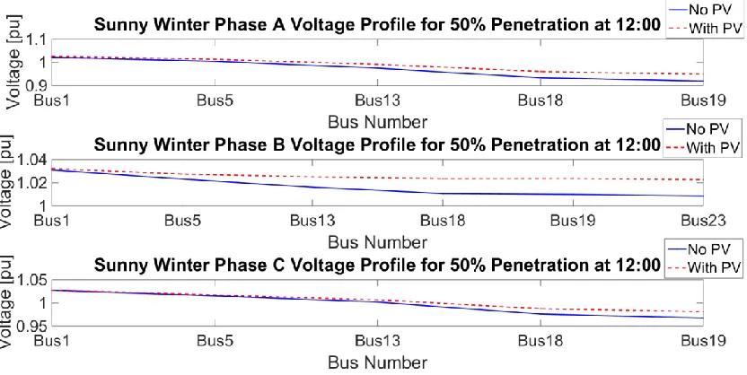
Figure 3-8 shows the daily voltage fluctuation in summer and Figure 3-9 shows the daily voltage fluctuation in winter. The following observations are made:

 After PV is added, the voltage of a load node will increase. This is because when the load is supplied by solar power, the current on the feeder from the substation to the load will be reduced, which leads to a smaller line voltage drop.

 The further the load node is away from the substation, the larger the voltage rise is. This is because the voltage increase at the end node equals to the sum of the voltage increase at each upstream load node. Table 3-1 shows the maximum voltage rise at each node in different conditions.

 The voltage rise after PV is installed are more significant in winter. On a hot summer day, the load peaks at noon which coincide the PV generation peak so the installation of PV at load nodes will not be very significant. But in winter, the peak load happened in morning and early evening, therefore the load is low when PV output is high. As a result, the voltage rise significantly.

 By comparing the voltage waveform among no PV case, 50% penetration PV case and 100% penetration PV case, we can see that when 50% PV is added, the voltage profile looks the best. When there is no PV in the feeder, there is a low voltage problem during daytime. And when the penetration level comes to 100%, there is a high voltage problem.

(41)

30 Figure 3-8 Daily voltage profile for nodes in sunny day in summer

(42)

31 Table 3-1 Maximum voltage rise for season case study

Distance (mile)

Summer max voltage rise (pu) Winter max voltage rise (pu) 50%

Penetration

100% Penetration

Bus2 Aph 2.91 0.0042 0.0081 0.0056 0.0108

Bus9 Aph 4.6 0.0099 0.0192 0.0126 0.0244

Bus12 Aph 4.61 0.0130 0.0253 0.0169 0.0328

Bus24 Aph 12.9 0.0292 0.0566 0.0388 0.0756

3.2.2 Unbalances among 3-phase Loads

(43)

32 Figure 3-10 Voltage profile along the feeder at 12:00 pm in summer for season case

(44)

33

3.2.3 Voltage Flicker

Figure 3-12 and Figure 3-13 show the flicker severity factor,

P

_st, for bus 24 phase A in summer and winter. The following observations are made:



P

st will increase when PV penetration increases. The value of

P

st is larger in winter than in summer.

 In a sunny day, PV power does not vary much. Thus, most of these values of

P

st are smaller than 0.1, which means that voltage flicker is not likely to occur regardless it is in winter or summer.

(45)

34 Figure 3-13 Daily

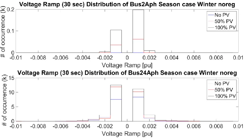
P

_st value of Bus24Aph in winter for season case

Figure 3-14 and Figure 3-15 show the distribution of 30-second interval voltage ramp. In order to look at is more clearly, all the points centralized around zero are excluded. Nevertheless, as it is a sunny day, all the voltage ramps still concentrate on very small values. Two nodes are picked up for each season, bus 2 locates at the beginning of feeder and bus 24 locates at the end of feeder. We can see that the voltage ramp for bus 24 distributes more widely than bus 2. So it shows us when PV is added, voltage variation of the feeder end will be influenced more seriously than feeder head. When we observe the same bus for different seasons, it is shown that winter voltage ramp is larger than that in summer. It means that comparing to summer,

(46)

35 Figure 3-14 Voltage ramp (30-second) distribution of nodes in summer for season case

Figure 3-15 Voltage ramp (30-second) distribution of nodes in winter for season case

3.3 Weather day study case

(47)

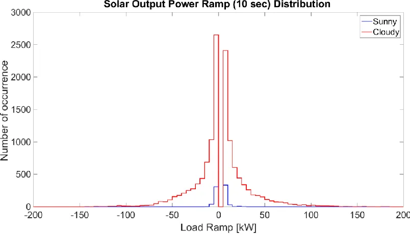
36 the peak PV power output is 4930 kW. The winter peak load for the feeder is 15300 kW (Table 1-1). Hence, this case represents 32% PV penetration. In cloudy day, if a cloud sweeps over this distribution feeder within a short period of time, the PV output variation is much larger than that in sunny day (Figure 3-16). On the other hand, these four zones are miles away from each other, the same solar irradiation cannot be gotten by all the zones at the same time. In order to make the simulation more realistic, we set a time delay among these zones as we mentioned in 2.1. The voltage profile and voltage flicker condition are compared between these two types of days.

Figure 3-16 Solar output power ramp comparison between sunny day and cloudy day

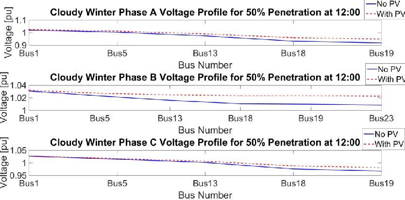
Figure 3-17 and Figure 3-18 show the voltage profile in sunny day and cloudy day. The following observations are made:

 In a sunny day, the voltage profile during day time is still very smooth. In a cloudy day the voltage varies a lot at the time cloud passing by. However, the day is sunny or cloudy will not influence the maximum voltage rise when the penetration percentage is the same, as shown in Table 3-2.

(48)

37 Figure 3-17 Daily voltage profile for nodes in sunny day in winter for weather case

(49)

38 Table 3-2 Maximum voltage rise for weather case study

Distance (mile)

Sunny day max voltage rise (pu) Cloudy day max voltage rise (pu) 50%

Penetration

Bus2 Aph 2.91 0.0063 0.0123 0.0062 0.0120

Bus9 Aph 4.6 0.0139 0.0270 0.0137 0.0265

Bus12 Aph 4.61 0.0177 0.0344 0.0174 0.0335

Bus24 Aph 12.9 0.0399 0.0776 0.0394 0.0752

Figure 3-19 and Figure 3-20 show the voltage profile along the whole feeder at 12:00 pm in sunny day and cloudy day. Since cloud passing by is a dynamic process, it will not influence the voltage drop trend for one snap shot. So there is no much differences between these two figures.

(50)

39 Figure 3-20 Voltage profile along the feeder at 12:00 pm in cloudy day for weather case

3.3.2 Voltage flicker

P

st value fluctuation for Bus 24 phase A. In this case, the

P

st values in sunny day and cloudy day are almost the same when there is no many clouds passing

by. Nevertheless, when clouds start to pass by more frequently from 8:00 am to 1:00 pm,

P

_st values in cloudy day will increase dramatically, which is almost the twice of that in sunny day.

A higher PV penetration percentage will also cause larger

P

st values. Thus, from the view of

st

P

value, voltage flickers are more likely to appear in cloudy days at nodes with high

(51)

P

_st value of Bus24Aph in winter for weather case

(52)

41 Figure 3-22 Voltage ramp (30-second) distribution of nodes in winter for weather case

3.4 Voltage flicker study

From the above simulation cases, it has shown that node at feeder end has the highest chance to suffer voltage flicker problem. This part will talk about for the feeder end nodes, what factors will influence the chance of occurring voltage flickers and how the voltage profile performs when these factors change.

As we mentioned above, the voltage flicker is caused by a big voltage variation in a short period of time. So it is essential to know what parameters in the feeder leads to voltage variation. If we look into the feeder from the end node, the equivalent circuit can be expressed by Figure 3-23 shows. The voltage variation 𝛥𝑉 for node at feeder end can be calculated by

𝛥𝑉 = 𝑅 ∗ 𝛥𝐼 (3-1)

(53)

42 Figure 3-23 Equivalent circuit for distribution feeder

In general, the current variation is determined by the net load change during that period time, and the equivalent resistance is determined by the length and impedance of each transmission line. Two simulation cases are set respectively to find how these two parameters impact the

voltage variation, or voltage flickers. The

P

st value and 10-second voltage variation are be used to judge the condition of voltage flickers in this part.

3.4.1 Current variation

(54)

43 a net load variation at all these nodes, along with a current variation along the feeder and voltage variation of the node at feeder end. Under this condition, this case will focus on comparing the voltage variation with different percentage PV penetrations in a cloudy day, which the current variation could be larger than sunny day.

Figure 3-24 Example for load variation possibility

In this simulation, the parameter of transmission lines are set to be constant value. Summer load profiles are considered as light load case, and winter load profiles represent heavy load case. The same PV profiles are added into these two cases. 5 kW PV capacity is installed at each house. As Table 2-5 shows, there are 1532 houses in the whole feeder, which means that 7660kW PV is added. In order to have more comparison, the situation for 2.5 kW PV per house (3830 kW in total) and 7.5 kW PV per house (11490 KW in total) are also simulated.

P

_st value for bus 24 phase A with different PV penetration percentage in a sunny summer, a sunny winter, a cloudy summer and a cloudy winter. From

this figure it is shown that in sunny day,

P

st values are more stable during daytime. And in

cloudy day,

P

st values will become extremely higher when clouds passing by. The values keep very small when no PV is added, which proves that the change of customer load will not impact it much.

Table 3-3 shows the maximum

P

st value during a day of different conditions. The maximum values are nearly zero when there is no PV. When the feeder shares the same solar irradiation

(55)

44 almost the same no matter it is light load or heavy load case. With the penetration percentage

increases, the maximum value of

P

_st will increase with the same multiple growth.

Figure 3-25 Daily

P

_st value of Bus24Aph in winter for flicker study (current variation)

Table 3-3 Maximum

P

_st value for flicker study (current variation)

Daily Maximum

P

_st value

No PV 2.5kW/house 5kW/house 7.5kW/house

Sunny Summer 0.00032 0.022 0.040 0.068

Winter 0.00054 0.026 0.058 0.069

Cloudy Summer 0.00032 0.039 0.072 0.121

Winter 0.00054 0.047 0.085 0.116

Figure 3-26 shows the 10-second voltage ramp distribution of bus 24 phase A for different cases. In order to make the figure more intuitive, all the voltage ramp values distributed around zero are eliminated as they will not cause problems. From the distribution histogram it is shown that in sunny day the voltage ramp is pretty small, and in cloudy day the values distribute more

widely. Similar to the

P

st value, light load or heavy load does not impact the voltage ramp distribution. It further proves that customer load change will not have a big impact on leading to voltage flickers.

(56)

45 the same penetration level and the same solar irradiation pattern, the difference is very small, almost can be ignored. And the maximum voltage ramp value increases with the same multiple growth of the increase of PV penetration percentage.

Figure 3-26 Voltage ramp (10-second) distribution of Bus24Aph for flicker study (current variation)

Table 3-4 Maximum voltage ramp value for flicker study (current variation)

Daily Maximum Voltage Ramp (10 second, absolute value)

No PV 2.5kW/house 5kW/house 7.5kW/house

Sunny Summer 0.0003 0.0023 0.0042 0.0069

Winter 0.0010 0.0027 0.0049 0.0067

Cloudy Summer 0.0003 0.0200 0.0372 0.0559

Winter 0.0010 0.0252 0.0439 0.0603

From the observations above, customer load change will not impact voltage flicker appearance. Even after PV is added, it still does not impact a lot in sunny day. Only when there are many clouds passing by the voltage flickers will have a higher chance to appear. The higher PV

(57)

46

3.4.2 Feeder resistance

The impedance of the whole feeder is consist of two parts, the first is the impedance of transmission lines and the second is the impedance from the load. Nevertheless, in our simulation the load profile for each node is already fixed, and all the nodes with load are set to be PQ bus. Therefore, the only impedance we can change is the transmission lines’ impedance. The way we control it is to increase the length of every line without changing any other line parameters. Three types of feeder are constructed in this part. The first one is the feeder with original line length, the line length in the second feeder is 1.5 times as much as the original one and the line length in the third feeder is 2 times as much as the original one. All these three feeders are simulated with summer and winter load profile, no PV case and 5kW cloudy PV per house case are considered for each season.

P

_st value fluctuation for each case. When there is no PV, the

P

_st values are around zero in both summer and winter, and the values do not vary a lot for different

line length. In cloudy day the

P

st values become larger. The longer the transmission lines are,

the higher

P

st values are. Comparing to other two

P

st patterns in winter, an extremely increase

for daily

P

st value is observed when the line has two times as much as original length.

Table 3-5 shows the maximum

P

st value for different cases. It is shown that when the feeder

with cloudy day PV has original length and 1.5 times length, their maximum

P

st value are still almost the same. However, when the length of each transmission line extends to two times, the

(58)

P

_st value of Bus24Aph in winter for flicker study (feeder resistance)

Table 3-5 Maximum

P

_st value for flicker study (feeder resistance)

Daily Maximum

P

_st value

Original Length Length*1.5 Length*2

No PV Summer 0.0003 0.0006 0.0008

Winter 0.0005 0.0009 0.0010

5kW/house Cloudy

Summer 0.0719 0.1155 0.1713

Winter 0.0845 0.1314 0.2874

Figure 3-28 shows the 10-second voltage ramp distribution of bus 24 phase A in different cases, all the occurrence distributed around zero are eliminated. It is shown that when there is no PV, all the voltage ramps are concentrate around zero no matter how long the transmission lines are. And when cloudy PV is added, the feeder length will begin to impact the voltage ramp distribution. The longer the feeder is, the more extensive the voltage ramp distribution is.

Table 3-6 shows the daily maximum voltage ramp value. All the maximum 10-second voltage ramp are nearly zero when no PV is installed. In cloudy day, the maximum value will increase with the extension of feeder length. With the same feeder length, the largest voltage ramp in winter is always larger than that in summer. The difference between summer and winter will increase with the increase of feeder length.

(59)

48 Figure 3-28 Voltage ramp (10-second) distribution of Bus24Aph for flicker study (feeder

resistance)

Table 3-6 Maximum voltage ramp value for flicker study (feeder resistance)

Daily Maximum Voltage Ramp (10 second, absolute value)

Original Length Length*1.5 Length*2

No PV Summer 0.0003 0.0005 0.0007

Winter 0.0010 0.0023 0.0025

5kW/house Cloudy

Summer 0.0372 0.0553 0.0776

Winter 0.0439 0.0898 0.1436

From the

P

_st value comparison and 10-second voltage ramp comparison in all the above cases, it can be concluded that feeder impedance will not impact voltage flicker situation when there is no PV in the distribution system. Nonetheless, in cloudy day the voltage flickers are more likely to appear when the line impedance is large. On the other hand, with the same PV penetration percentage, peak load condition is affected more severely by feeder length than light load condition.

3.5 Zonal case

(60)

49 condition. 5kW PV capacity is added at each house. We will focus on observing the voltage profiles of these cases. In this way we can find the different effect on the voltage profile at each node with the installation of PV in different areas.

Figure 3-29, Figure 3-30, Figure 3-31 and Figure 3-32 show the daily voltage profiles of bus 2 phase A (locates at zone 1), bus 9 phase A (locates at zone 2), bus12 phase A (locates at zone 3) and bus 24 phase A (locates at zone 4) in different cases. Table 3-7 and Table 3-8 show the maximum voltage rise for each case. Following observations are made:

 It is shown that for bus 2 phase A which locates in zone 1, its voltage affect order from strong to weak is PV at zone 3, zone 1, zone 4 and zone 2. Zone 3 has the strongest impact because it has the largest number of houses locate at phase A. Therefore, the solar power generated for phase A will be large and leads the maximum voltage rise to node at zone 1 even they are not nearby. Zone 1 has the second strongest impact because the PV panels are directly installed at Bus2Aph. The reason for zone 4 has a stronger impact than zone 2 is house locates at phase A in zone 4 is more than that in zone 2.

 For bus 9 phase A which is located in zone 2, zone 2 and zone 3 almost have the same impact because of the larger PV power output in zone 3 and the nearer distance in zone 2. The impact for zone 1 is very small as zone 1 is located before zone 2.

 For bus 12 phase A which is located in zone 3, zone 3 has a definitely largest impact since it has most houses at phase A and PV is directly installed there. Zone 4 has the second largest influence because it locates after zone 3. The impact from zone 1 and zone 2 can be almost ignored by comparing with the impact from other two zones.

(61)

50 Figure 3-29 Daily voltage profile for nodes in sunny day in summer for zonal case

(62)

51 Table 3-7 Maximum voltage rise in sunny day for zonal study

Maximum voltage rise after 5kW PV/house added in sunny day

Zone 1 Zone 2 Zone 3 Zone 4

Summer Bus2Aph (Zone 1) 0.0031 0.0009 0.0043 0.0023

Bus9Aph (Zone 2) 0.0008 0.0111 0.0111 0.0062

Bus12Aph (Zone 3) 0.0008 0.0038 0.0220 0.0113

Bus24Aph (Zone 4) 0.0008 0.0039 0.0247 0.0647

Winter Bus2Aph (Zone 1) 0.0032 0.0011 0.0063 0.0047

Bus9Aph (Zone 2) 0.0009 0.0117 0.0145 0.0109

Bus12Aph (Zone 3) 0.0010 0.0043 0.0270 0.0183

Bus24Aph (Zone 4) 0.0011 0.0048 0.0337 0.0879

(63)

52 Figure 3-32 Daily voltage profile for nodes in cloudy day in winter for zonal case

Table 3-8 Maximum voltage rise in cloudy day for zonal study

Maximum voltage rise after 5kW PV/house added in cloudy day

Zone 1 Zone 2 Zone 3 Zone 4

Summer Bus2Aph (Zone 1) 0.0031 0.0008 0.0044 0.0023

Bus9Aph (Zone 2) 0.0008 0.0110 0.0111 0.0063

Bus12Aph (Zone 3) 0.0008 0.0038 0.0221 0.0114

Bus24Aph (Zone 4) 0.0008 0.0038 0.0249 0.0660

Winter Bus2Aph (Zone 1) 0.0032 0.0011 0.0064 0.0053

Bus9Aph (Zone 2) 0.0010 0.0120 0.0149 0.0119

Bus12Aph (Zone 3) 0.0010 0.0044 0.0276 0.0197

Bus24Aph (Zone 4) 0.0012 0.0049 0.0344 0.0903

In conclusion, from the observations above, we can find that the PV output capacity and the distance between PV site and nodes are the two most significant factor to quantify the impact to voltage profile. Also, PV will not impact much to nodes after the installation location. In this feeder, if we want to choose one zone to install PV in order to improve voltage profiles for the whole feeder, zone 3 is the best choice.

3.6 Commercial load case

(64)

53 compare the results with the residential load, PV capacity keeps the same. The feeder map for this case is shown in Figure 3-33.

Figure 3-33 Feeder map for commercial load case

(65)

54 Figure 3-34 Load profile of Bus24Aph in winter for commercial case

3.6.1 Commercial load and residential load

(66)

55 Figure 3-35 Voltage profile in sunny winter for commercial load case

Figure 3-36 Voltage profile in cloudy winter for commercial load case

P

st value comparison between residential load and commercial

load. For all of these cases, commercial load condition has a larger daily

P

st values. Table 3-9

(67)

P

_st value comparison between residential load and commercial load

Table 3-9 Maximum

P

_st value for residential load and commercial load

Daily maximum

P

st value

Residential Commercial

No PV 0.0005 0.0800

Sunny 0.0576 0.0721

Cloudy 0.0845 0.1026

(68)

57 Figure 3-38 Voltage ramp (10-second) distribution comparison between residential load and

commercial load

Table 3-10 Maximum voltage ramp (10-second) for residential load and commercial load

Daily maximum voltage ramp (10 second) Residential Commercial

No PV 0.0010 0.0064

Sunny 0.0049 0.0062

Cloudy 0.0439 0.0509

Therefore, from the point of view for both

P

st value and voltage ramp, it can be concluded that commercial load is more likely to suffer voltage flickers than residential load in the same environment condition. The reason is the larger load variance for commercial load during daytime.

3.6.2 Distribution transformer

(69)

58 Table 3-11 Distribution transformer parameter

Distribution transformer

KVA 50

HZ 60

HV 22860

LV 240

(70)

59 Figure 3-39 Feeder map after distribution transformer added

(71)

60 supplies much of the load, so the current from grid will decrease, which leads to a smaller voltage drop.

Figure 3-40 Voltage profile comparison between without transformer and with transformer

Table 3-12 shows the maximum and minimum voltage difference between with transformer case and without transformer case. When there is no PV, the voltage drop on the transformer is between 1.95% and 5.73%. The maximum voltage drop happens at peak load time and the minimum voltage drop happens at light load time. After PV is added, the voltage drop range decreased, which is from 1.36% to 5.7%. The maximum drop occurs in the evening, which is the time the sun goes down and the PV output becomes zero. The load at that time is still heavy, so the voltage drop is large. The minimum voltage drop occurs in the morning, the time with light load but large PV output. Hence, integrating PV helps reduce the voltage drop on transformer.

Table 3-12 Voltage difference between with transformer case and without transformer case

Voltage difference Time

Without PV Maximum 0.0573 11:30 am

Minimum 0.0195 2:15 am

With PV Maximum 0.0570 6:16 pm

(72)

61

Chapter 4

Conclusion and Future Work

In this thesis, a utility distribution feeder is simplified to a feeder with a source, transmission lines and loads. Then, the load data and PV data are processed to fit our simulation requirement. After that, several cases are simulated in OpenDSS and MATLAB. Finally, by using the voltage profiles we get from simulation, daily voltage pattern and voltage flicker condition in different cases are analyzed and evaluated.

The contributions of the thesis are summarized as follows:

 Developed a methodology to disaggregate residential load. By using this method the total load at each node can be resolved to a set of customer houses’ load profiles. The sum of these load profiles will still meet the feeder parameter. PV can also be

installed according to the number of houses at each node.

 A PV output time delay is set among different zones to simulate the situation that each node will not see the same solar irradiation at the same time because of the long distance.

 Revealed the daily voltage fluctuation and voltage flicker condition in different seasons, different weather conditions, different PV penetration percentages, different PV installation locations and different load types.

 Analyzed two factors which will influence the voltage flicker condition in a distribution feeder, current variation and feeder resistance. Simulations are done to prove the inference.

Our future work will focus on the following directions:

 Develop a reasonable way to interpolate 15-minute load data to 1-second load data.

 Develop a way to create more diversified PV output for each house.

 Do the simulation in another actual feeder without simplified to see if the results are still correct in a large distribution system.

(73)

62

References

[1] Shapiro, Gary. "America's Comeback Starts with American Innovators [Soapbox]." IEEE Consumer Electronics Magazine 1.1 (2012): 19-24.

[2] Lazzeroni, Paolo, et al. "Impact of PV penetration in a distribution grid: A Middle-East study case." Research and Technologies for Society and Industry Leveraging a better tomorrow (RTSI), 2015 IEEE 1st International Forum on. IEEE, 2015.

[3] Ren, P. S. "Renewables 2015 global status report." REN21 Secretariat: Paris, France (2015).

[4] Solangi, K. H., et al. "A review on global solar energy policy." Renewable and sustainable energy reviews 15.4 (2011): 2149-2163.

[5] http://www.rechargenews.com/wind/1431228/duke-energy-raises-2020-renewable-energy-target-to-8gw

[6] Thomson, M., and D. G. Infield. "Impact of widespread photovoltaics generation on distribution systems." IET Renewable Power Generation 1.1 (2007): 33-40.

[7] Key, T. "Distributed photovoltaics: Utility integration issues and opportunities." Electric Power Research Institute, Tech. Rep (2010).

[8] Turitsyn, Konstantin, et al. "Options for control of reactive power by distributed photovoltaic generators." Proceedings of the IEEE 99.6 (2011): 1063-1073.

[9] Ballanti, Andrea, and Luis F. Ochoa. "On the integrated PV hosting capacity of MV and LV distribution networks." Innovative Smart Grid Technologies Latin America (ISGT LATAM), 2015 IEEE PES. IEEE, 2015.

[10] http://www.nrel.gov/gis/solar.html

[11] Thomson, Murray, and David G. Infield. "Network power-flow analysis for a high penetrat

Analysis of Voltage Problems for PV Integrated Distribution Feeder.

ABSTRACT

DEDICATION

ACKNOWLEDGEMENTS

TABLE OF CONTENTS

LIST OF TABLES

LIST OF FIGURES

Chapter 1

1.1 Background

1.2 PV Integration Issues

1.3 Data Preparation

Branch # From To Phase Length (mile) Impedance ( ohm/mile) Line Type

Node # Phase Node Type Power Factor Other Information

Load Location Winter Peak Load (kW) Winter Reactive Power (kVAR)

1.3.2 Residential Load Data

1.3.3 Solar data

1.3.4 Modeling Air Conditioning Loads

Chapter 2

2.1 Feeder Network Model Setup

Zone 1 Zone 2 Zone 3 Zone 4

Bus# Winter peak load (kW) House# Consumption/House (kW)

Bus# Winter peak load (kW) House# Consumption/House (kW)

2.2 Load Data Interpolation

2.3 PV installation

Chapter 3

3.1 Base Case

3.1.2 Voltage Flicker

3.2 Season Study Case

Distance (mile)

3.3 Weather day study case

Distance (mile)

3.3.2 Voltage flicker

3.4.1 Current variation

Daily Maximum

Daily Maximum Voltage Ramp (10 second, absolute value)

3.4.2 Feeder resistance

Daily Maximum

Daily Maximum Voltage Ramp (10 second, absolute value)

Maximum voltage rise after 5kW PV/house added in sunny day

Maximum voltage rise after 5kW PV/house added in cloudy day

3.6 Commercial load case

Daily maximum

3.6.2 Distribution transformer

Voltage difference Time

Chapter 4

References