Advancing Connected Vehicle Technologies by Improving Vehicular Channel Model Accuracy and Safety Performance Measures.

(1)

ABSTRACT

CARPENTER, SCOTT. Advancing Connected Vehicle Technologies by Improving Vehicular Channel Model Accuracy and Safety Performance Measures. (Under the direction of Dr. Mihail L. Sichitiu).

Wireless communications technologies allow vehicles to exchange information and thus create connected vehicle networks that enable safety applications, such as accident avoidance, thereby reducing damage and injuries caused by moving vehicle collisions. The most promising technologies in the U.S. that will enable such a vehicular ad hoc network (VANET) are collectively referred to as Dedicated Short-Range Communications (DSRC). While standards evaluation units exist, deployment has been limited to prototype testing, forcing VANET researchers to rely on simulation tools and supporting models, with mixed results. Results from inaccurate models can threaten the evaluation of safety applications, with existing performance metrics often only evaluating communications Quality of Service (QoS) measures while ignoring vehicular mobility.

(2)

(3)

(4)

Advancing Connected Vehicle Technologies by Improving Vehicular Channel Model Accuracy and Safety Performance Measures

by Scott Carpenter

A dissertation submitted to the Graduate Faculty of North Carolina State University

in partial fulfillment of the requirements for the degree of

Doctor of Philosophy

Computer Science

Raleigh, North Carolina 2018

APPROVED BY:

_______________________________ _______________________________

Dr. Mihail L. Sichitiu Dr. David Thuente

Committee Chair

_______________________________ _______________________________

(5)

DEDICATION

(6)

BIOGRAPHY

(7)

ACKNOWLEDGMENTS

This dissertation is the culmination of roughly 6 years of my mostly part-time education at the North Carolina State University (NCSU). My experiences at NCSU during this wonderful time have played an important part in my growth, intellectually, and as a person. I would like to use this opportunity to thank those who have affected me during this time and assisted me in this growth.

First and foremost, I would like to thank my advisor, Dr. Mihail L. Sichitiu, for his exceptional guidance and support over the course of my time pursuing this degree. At our first meeting, Dr. Sichitiu asked me “Why do you want a Ph.D.?”. I don’t recall my assuredly pitiful answer. But, I will forever remember Dr. Sichitiu’s response, “No, that’s not a good reason for a Ph.D.”. I quickly realized this was someone who was actually going to make me learn something, not only in an educational sense, but through a journey to learn about myself. I always looked forward to our multitude of meetings, as I came to realize Dr. Sichitiu practices an amazing balance of technical explanation, challenging questions, constructively thorough and helpful comments, humor, and just at the right times, enough silence to allow me to learn. I am forever grateful that he allowed me to be one of his graduate students, and I owe the successful completion of my Ph.D. entirely to Dr. Sichitiu’s mentoring. I also believe I owe him several boxes of red pens to replace his supply, but that is another matter altogether.

Over the course of my years in graduate school at NCSU, I have had the benefit of interacting with faculty and staff who have substantially influenced my research with their broad insights and interesting perspectives. I would like to thank the members of my doctoral committee, Dr. David Thuente, Dr. Rudra Dutta, and Dr. Raju Vatsavai for their valuable feedback during the course of my degree. Additionally, I would like to thank the faculty that clarified for me the complexities of many topics and continually challenged me to understand them in ways I would never have otherwise imagined, specifically, Dr. Do Young Eun, Dr. Munidar Singh, Dr. Edgar Lobaton, Dr. Aldo Dagnino, Dr. Douglas Reeves, Dr. George Rouskas, Dr. Laurie Williams, Dr. Wenye Wang, Dr. Khaled Harfoush, Dr. Purush Iyer, and Dr. Javad Taheri. Go Pack!

(8)

Michael Young, Dr. Camille Barot, Dr. Sarah Heckman, Dr. David Sturgill, Carol Allen, Linda Honeycutt, and Terri Martin-Moss. I would also like to thank those Computer Science students that braved the hot, summer months in Raleigh and allowed me the pleasure of teaching them about data structures and operating systems. These classroom interactions were indeed some of my fondest and most rewarding experiences while at NCSU.

I would like to thank the collaborative members of the ns-3 simulator framework, who guided me in developing much of the code that was eventually contributed, especially Dr. Tom Henderson, Dr. Peter Barnes, Dr. Tomasso Pecorella, Dr. George Riley, and Dr. Konstantinos Katsaros. Additionally, I would like to thank the members of the SAE DSRC Technical Committee, who helped me tremendously in understanding the DSRC operational standards and their intent, especially Dr. Jim Misener and Dr. Sue Bai.

While this body of work was created through many hours spent at home and at libraries, it also resulted in the consumption of what I am sure has been hundreds of gallons of caffeinated beverages, mostly coffee. And much of that consumption was done in the soft, Wi-Fi glow of various coffee shops and fast food establishments. I extend my warmest thanks to all those in the service industry who unknowingly contributed to helping me maintain my focus through copious consumption of caffeinated concoctions while I spent many hours enjoying the fine atmosphere of their establishments.

(9)

(10)

LIST OF TABLES

Table 2.1 DSRC device classes and operating parameters……… 13 Table 2.2 Safety-related vehicle communications applications (adapted from [1]).. 33 Table 2.3 V2V safety communications applications with greatest potential safety

benefit……… 35 Table 2.4 Communications requirements for three CAMP/VSCC safety

Applications………... 36

Table 3.1 Scenario topology parameters………49

Table 3.2 Network simulation parameters………. 53

Table 3.3 PDR average and standard deviation for three fading models…………... 59 Table 4.1 Trip data summary for Safety Pilot Model Deployment Data

Environment. Over 22,000 vehicular trips covering 167,000 km in 4,700 hours resulted in more than 48M BSMs that were successfully received……….……… 65 Table 5.1 Five vehicular channel models for which estimated PRR is compared

to the actual large-scale SPMD measurement data……….. 80 Table 5.2 Parametric values for the VCMs. The MLE of each parameter is

shown with statistical bias in parentheses and appropriate units in

brackets………...…81 Table 5.3 Numerical results for the RSME of three metrics (PRR, IPG, and

CRRL) for five VCMs as compared to the Ann Arbor SPMD test data set. As expected, the unit disk model performs poorly in predicting PRR. While all other models better predict PRR, they fail to accurately predict consecutive packet losses (i.e., IPG) and reception (i.e., CRRL). Use of geodata to deterministically estimate path loss through obstacles (i.e., Model E) improves CRRL, as compared to a purely stochastic model (i.e., Model B) that does

not make use of such geodata……….…….. 87 Table 5.4 Summary of five stochastic and/or deterministic VCMs evaluated

against the Ann Arbor SPMD data set………. 88

Table 6.1 Expected run lengths and gap lengths for five distance bins. Expected run length increases when distance between transmitting and receiving vehicles decrease. Contrastingly, expected gap

(14)

Table 6.2 Expected PRR for five distance bins. PRR decreases as distance

between transmitting and receiving vehicles increases………..99 Table 6.3 Numerical results of the RSME for three metrics – PRR, IPG, and

CRRL – of the combined dual-slope distance-breakpoint model with the BUR-GEN burst distribution function (i.e, Model F,

compared to five common (i.i.d. only) VCMs (i.e., Models A-E)…….. 118 Table 7.1 Three message dissemination strategies that are evaluated………. 131 Table 7.2 Four configuration that vary forwarding zone parameters based

on different application requirements……….. 134 Table 8.3 Application range and message tolerance for four VSC safety

Applications………. 147 Table 8.4 Minimum and maximum safety performance requirements used for

(15)

LIST OF FIGURES

Figure 2.1 Total U.S. motor vehicle fatalities per 100,000 population,

1950 – 2012………10

Figure 2.2 DSRC reference model………...12

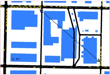
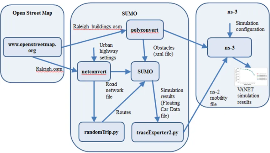
Figure 2.3 Representative VANET simulation tools. Adapted from: [1]…………...31 Figure 3.1 Obstacles in a downtown Raleigh, NC scenario as simulated in

SUMO……… 42 Figure 3.2 Obstacle shadowing model enhancements to the ns-3 reference model… 43 Figure 3.3 A subset of buildings data for the downtown Raleigh, NC USA area…... 44 Figure 3.4 Pseudo-code for the algorithm that determines the number of

obstacle wall intersections and obstructed distance between two points... 45

Figure 3.5 Obstacle intersection range……… 46

Figure 3.6 Process flow for experimental setup……….. 48 Figure 3.7 View in GoogleEarth™ (above) and visualization in SUMO of

Open Street Map (OSM) buildings data (below) for an open

highway scenario near Raleigh, NC USA………. 50 Figure 3.8 View in GoogleEarth™ (above) and visualization in SUMO of

Open Street Map (OSM) buildings data (below) for a residential

neighborhood scenario near Raleigh, NC USA………. 51 Figure 3.9 View in GoogleEarth™ (above) and visualization in SUMO of

Open Street Map (OSM) buildings data (below) for an urban

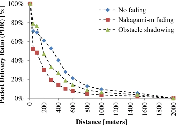
downtown scenario near Raleigh, NC USA………...52 Figure 3.10 Example propagation loss effects near an intersection……….. 54 Figure 3.11 PDR over time for three fading models………. 55 Figure 3.12 PDR for the open highway scenario with 250 vehicles, for three

different fading models as a function of the distance from the

transmitter………...56 Figure 3.14 PDR for the downtown scenario with 250 vehicles, for three

transmitter……….. 57 Figure 3.13 PDR for the neighborhood scenario with 250 vehicles, for three

(16)

Figure 3.15 PDR for residential neighborhood scenario with no fading, for 50 – 250 vehicles as a function of the distance from the

source of the transmission………. 58 Figure 3.16 CPU-time (minutes) of the sum of times to simulate 2000s of

150 vehicles in the highway, residential, and downtown scenarios

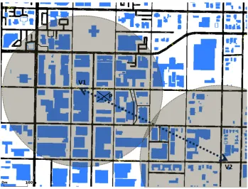
for different fading models……… 60 Figure 4.1 Representative coverage area for the Safety Pilot Model

Deployment in Ann Arbor, Michigan. Highlights represent the line of sight of over 3 million successful BSM receipts for selected encounters between a receiving vehicle (Rx) and a

transmitting vehicle (Tx), as derived from the SPMD DE……….64 Figure 4.2 Packet reception for four example encounters from the SPMD

DE. Encounter time can vary significantly. When vehicles are in close proximity to one another, packet reception is more

likely, but the correlation to distance is otherwise inconsistent………… 67 Figure 4.3 Packets received (red, below) relative to packets not received

(green, above) as a function of the distance between sender and receiver for the SPMD DE. Reception success (i.e., PRR) decreases as distance increases. PRR is greater than 65% only at distances less than 10m and decreases rapidly with distance, with

few packets successfully received beyond 400m………...68 Figure 4.4 Average IPG as a function of relative transmitter distance from

the receiver as centered at (x=0, y=0). IPG is generally low regardless of senders being directly ahead of or behind the receiver, but increases as distance increases, especially when lateral distances increase and the transmitter is behind the receiver. Numbers indicate the count of IPG values that are

averaged for each cell……… 69 Figure 4.5 Log-log plot of the probability distribution of frequency of

inter-packet gaps in seconds, out to one minute, within the

SPMD DE. A majority (93%) of IPG lengths are less than 200ms (i.e., losses of 0 or 1 packet), while longer IPG lengths plausibly

follows a power law distribution model, p(x)=0.342x-2.374……… 70 Figure 4.6 Overlapping Allan deviation, ( ), of packet loss gaps throughout

Ann Arbor, as a function of , the averaging factor in seconds. The SPMD DE dataset is split into four quartiles (i.e., Q1..Q4) by the

average gap length for 1950 encounters……….73 Figure 5.1 The receiving vehicle, RX (green trajectory), moves from the top

right to the left, while the transmitting vehicle, TX (blue trajectory), moves from the top middle to the bottom middle and enters a

(17)

in this encounter. Here, the packet losses do not seem to correspond to building or parking deck obstacles between vehicles. It is possible that the losses are caused by trees, elevation changes, and/or trucks or other vehicles coming between sender and receiver, but there is insufficient data from which to definitively and deterministically

derive path loss in this encounter………... 78 Figure 5.2 Geodata from Open Street Map (OSM) (a) for a section of the

Ann Arbor area, and the equivalent view from Google Earth (b). Maroon areas represent geodata from OSM for various types of buildings, and blue areas represent parking decks, lots, and parks, all of which OSM treats homogenously as 2D outlines. Geodata is missing for many structures present in Ann Arbor and does not account for all obstacles that may occur between vehicles traveling

the streets………79 Figure 5.3 PRR for log-scale distance from 5-500m for five VCMs. PRR

predictions vary greatly among the models. Stochastic

lognormal-based models B and C favorably predict PRR as does

model E that deterministically accounts for obstacle shadowing………...83 Figure 5.4 Log-log scale of the pdf of inter packet gap (IPG) as a function

of gap length out to 60s. The results for the i.i.d.-assuming model differ greatly from the power-law fitting test data, indicating that such models do not predict well the packet gap distributions found

in the field test data of the SPMD……….. 84 Figure 5.5 Log-log scale of the pdf of consecutive reception run-length

(CRRL) as a function of time out to 60s……… 85 Figure 5.6 The average number of obstacle walls penetrated (left axis) and

the average total distances traveled within them (right axis) as a function of total distance between vehicles, based on the SPMD test data set and geodata available from OSM. As expected, there are few obstacles between vehicles when they are close together, while the average obstacle interior distances traveled is approximately 10% of the total distance between vehicles,

up to about 800m………... 86 Figure 6.1 Relative velocity between two vehicles is a function of the

individual vector velocities of the vehicles and the angle

(18)

Figure 6.2 The pdf of relative velocity of vehicles during V2V communications encounters throughout the Ann Arbor-based Safety Pilot Model Deployment. Over half of the time vehicles move relative to one another less than 5 m/s, indicating that vehicles during encounters are stopped or following one another at similar speeds. The

encounter data shows that there are few times when relative velocity is greater than 20 m/s, and there were no incidences of relative

velocity of more than 60 m/s.………..95 Figure 6.3 The communications pattern of an illustrative V2V encounter within

the SPMD test data set of the inter-vehicle distance versus

time. Packet receptions within 200m are bursty, and interspersed with inter-packet gaps. Communications is highly asymmetric with respect to distance, as there are no receptions after =32 , when the vehicles begin to separate away from one another. Prior to the receipt of the first packet, and after the reception of the last packet, there are long gaps of no receptions, even though the vehicles are

quite close to one another………...96 Figure 6.4 The log-log scale pdf of IPG and CRRL, respectively, within the

SPMD test data set. Both IPG and CRRL follow power-law

distributions………97 Figure 6.5 The cdf of IPG and CRRL, respectively, within the SPMD test data

set. In both plots, the x-axis is log-scale. A majority of packet gaps are very short, with 95% of all gaps less than 11 packets (i.e., 1.1s). Although the analysis was limited to a maximum gap length of 600 packets (i.e., 60s), approximately 1.5% of all gaps are ≥ 600 packets. Consecutive runs of packet receptions are also typically short, with 95% of all runs being less than 11 packets in length (e.g., 1.1s). Long bursts of consecutively received packets are very rare, with no runs of more than 200 consecutive packets……….98 Figure 6.6 The CPDF of gap and run lengths for the SPMD test data set

and a 5PLR estimation model. The probability of a gap ending or a run length continuing are not independent of the previous gap / run length history, indicating that bursty reception and loss behaviors within the environment are not the result of an

i.i.d. packet generation phenomenon………... 101 Figure 6.7 5PLR models of the CPDF of gaps < 1.2s and runs < 7.5s,

for four distance bins. Conditional probabilities for short gaps and runs (e.g., lengths of 1-2) differ as a function of distance, but are nearly identical for other gap and run lengths,

(19)

Figure 6.8 5PLR models of the CPDF of gaps < 1.2s and runs < 7.5s, for five different temporal subsets of the SPMD test data set. Conditional probabilities for short gaps and runs (e.g., lengths of 1-2) differ among the temporal data sets, but are nearly identical for other gap and run lengths, independent of the

temporal subsets………... 103 Figure 6.9 The 2-state Markov chain Gilbert-Elliott Packet Loss Model…………. 105 Figure 7.10 Two binary streams, S1 and S2, that illustrate packet

generation results with equivalent PRR but different packet gap

and consecutive runs……….106 Figure 6.11 Architecture and data flow diagram for a packet generation

and evaluation model. A Flow Stream Analyzer is used to evaluate the PRR, IPG, and CRRL of the SPMD test data. The resulting distributions are used as inputs into a Burst Generator model that the Packet Generator combines with a path loss model to produce a modeled Flow Stream of alternating gaps and runs of packets. The model results are also analyzed by a Flow Stream Analyzer and the results of the test data and model

are compared……… 108 Figure 6.12 The inverse transformation method………. 109 Figure 6.13 Comparison of average PRR and expected PRR. Average PRR

(i.e., using the dual-slope distance-breakpoint path loss model derived from the SPMD test data) decreases smoothly as distance increases, while expected PRR drops in a stepwise

manner consistent with the distance bins used for their evaluation. Expected PRR is calculated using the subset of data points

that occur only during active communications, while the average PRR includes all data points throughout an entire encounter. As expected PRR excludes long periods of leading and trailing packet gaps, the value of expected PRR often exceeds that of

the path-loss-modeled average PRR……… 110 Figure 6.14 Sensitivity of 1− as compared to expected gap length. Expected

gap length increases as distance increases. However, since leading and trailing long packet gaps are excluded from the calculation of expected gap, the resulting expected PRR is higher than desired average PRR. By injecting long packet gaps into a packet stream with frequency 1− , expected PRR can be related to average PRR. The need for such injections is infrequent as short

distances, and increases as distance increases………. 113 Figure 6.15 The BUR-GEN (burst generator) packet stream generator

(20)

that consists of alternating gaps and runs that are drawn from gap and run burst distribution functions (i.e., line 15 and 19, respectively). With probability 1− ,, a long burst of length of

lost packets is injected into the stream………. 114 Figure 6.16 Simulation parameters. Vehicle mobility is modeled as

randomly generated V2V encounters. Path loss is modeled using the dual-slope distance-breakpoint model and using the “best fit” parameters identified in Chapter 5. The i.i.d. packet burst

generation Model C is evaluated against a model that includes

the BUR-GEN algorithm (i.e., Model F)………. 115 Figure 6.17 PRR comparison of the dual-slope distance-breakpoint model

(only) and the combined dual-slope distance-breakpoint model

with the BUR-GEN burst generation model……… 117 Figure 7.1 Conceptual view of the safety system in which vehicle A desires to

target safety messages towards the geocast region (GR) centered at v with radius RGR, requiring messages to be relayed through

the entire forwarding zone (FZ) that covers the entire area………. 124 Figure 7.2 An example timing diagram for the beaconcasting VANET…………... 126 Figure 7.3 Pseudocode (based on [12] for broadcast flooding. Line 1 receives

a message, m; line 2 decides if m should be forwarded; line 3 generates a new message, m’, by potentially amending the original message, m; line 4 determines the time at which the message should be resent; and line 5 schedules the rebroadcast of the

amended message m’ at some future time, t……… 127 Figure 7.4 Pictorial illustration of geocast regions for four configurations

(i.e., A, B, C, and D) that represent different application

requirements. The vehicle transmitting a BSM is located at the point labeled v and is assumed to be moving left to right at

approximately 20 m/s………... 133 Figure 7.5 Vehicular density (a) for a subset of the configuration space,

where darker-colored regions indicate areas through which more vehicles have traveled, and average BRR (b-e) for two different subsets of the scenario space and two different configurations (B and C), where darker-colored regions indicate higher BRR. Average BRR between scenarios is localized and may improve

(e.g., (c) vs. (b)), or degrade (e.g., (e) vs. (d))………. 136 Figure 7.6 A comparison for four different scenarios of the total number of

distinct tagged BSMs that are received, as a function of distance between the vehicle that originates the tagged BSM and

(21)

Figure 7.7 A comparison for four different scenarios of the averages of BRR as a function of distance between the vehicle that originally

transmits a BSM and vehicles that receive it………... 139 Figure 7.8 A comparison for four different scenarios of the averages

of awareness probability as a function of distance between

transmitting and receiving vehicles………. 140 Figure 7.9 A comparison for four different scenarios of the averages of

safety awareness probabilities as a function of distance between transmitting and receiving vehicles. Application requirements that increase forwarding zone coverage area help receiving vehicles that are likely to come in contact with one another improve

their safety awareness of the sending vehicle……….. 140 Figure 8.1 Packet reception for a subset of a V2V encounter derived from

the SPMD test data set for inter-vehicle separational distances less than 100m. Successful packet receptions are marked with a red “+”, and their absence indicates periods of packet loss.

Packet receptions and losses are bursty, and highly asymmetrical…….. 145 Figure 8.2 Awareness probability as a function of distance between

transmitter vehicle and receiving vehicle for maximum

safety tolerance requirements………...149 Figure 8.3 Awareness probability as a function of distance between

transmitter vehicle and receiving vehicle for minimum

safety tolerance requirements………...150 Figure 8.4 Numerical results of the RMSE of awareness probability

between the model and the SPMD Test Data, for maximum and

(22)

CHAPTER

1

INTRODUCTION

1

Chapter 1 Introduction

Collisions among moving vehicles lead all causes of traffic fatalities, injuries, and property damage [2]. By exchanging information using wireless communications, vehicles may employ both safety applications (e.g., accident avoidance), and non-safety applications (e.g., traffic congestion alerts) [3]. The US Intelligent Transportation Systems (ITS) Joint Program Office (JPO) suggests that vehicle safety applications and supporting technologies will prevent tens of thousands of automobile crashes every year [4]. The most promising technologies in the U.S. that will enable such a vehicular ad hoc network (VANET) are collectively referred to as Dedicated Short-Range Communications (DSRC).

While prototype testing thus far has been constrained to limited testbed environments, various vehicular and networking simulation tools assist VANET researchers by providing supporting functions from which to model a variety of environmental conditions. Despite the availability of such models, results are inconsistent and often do not accurately predict behaviors observed in real-world situations.

(23)

of VCMs and the resulting observations of packet loss behaviors. Furthermore, while many VCMs can predict somewhat accurately the packet loss rates observed in real-world deployments, they over-estimate inter-packet gap lengths greater than 0.2s and under-estimate the likelihood of runs of three or more consecutively and successfully received packets, potentially threatening the accuracy of packet-level performance when multiple safety messages much be received in short time windows.

Aside from the packet loss categorization that VCMs attempt, the notion of safety itself is endangered by the inconsistent data delivery requirements of safety applications. To be effective, different safety applications may each require distinct numbers of safety packets to be successfully received with varying latencies, presenting challenges in determining how to distribute the safety information to other vehicles and making it difficult to quantify the current value of safety. Evaluations that commonly consider information dissemination approaches that use geo-casting and flooding techniques often decline to include mobility considerations and do not focus on assessing safety efficiency in terms of safety application requirements.

This dissertation investigates VCMs and their impact to safety packet delivery and safety performance evaluations within especially challenging, realistic DSRC testbed environments.

1.1

Thesis Statement

By cooperatively communicating using DSRC technologies, a system of connected vehicles can improve situational awareness among drivers with the intent on improving driving safety and reducing automobile-related accidents.

The DSRC collection of standards includes IEEE Std. 802.11-2012 [5], IEEE Std. 1609/WAVE [6] [7] [8] [9] [10], and SAE J2735 Message Set Dictionary [11]. Modifications to the IEEE Std. 802.11-2012 [5] MAC and PHY layers (formerly known as IEEE 802.11p) allow every vehicle to rapidly broadcast information about itself (e.g., location, speed and heading) as a safety beacon (i.e., beaconcasting) to make other nearby vehicles aware of it so they can alert drivers of unsafe situations such as pre-crash scenarios.

(24)

scenarios, successful packet reception remains particularly challenging when numerous vehicles need to concurrently deliver safety messages in time-limited intervals under extreme environmental conditions. Packet losses in a VANET commonly result from separation distance, obstacles, and multi-path fading effects. Our analysis using an extensive experimental dataset collected from a deployment of approximately 3000 DSRC-capable vehicles operating around Ann Arbor, Michigan reveals that several common assumptions for DSRC (e.g., high packet reception rate for distances smaller than 100m) simply do not hold in real deployments.

Furthermore, accurate modeling of the vehicular channel endures as a challenging task. Vehicle-to-vehicle (V2V) channel attributes vary decidedly from those of traditional cellular channels, especially in terms of complicated propagation by-products from varying link variety, vehicle types, and environmental conditions, such as obstacles, that impact fading outcomes. Our results show that the DSRC deployment near Ann Arbor exhibits considerable shadowing and fading (i.e., sub-Rayleigh) events that challenge traditional VCM accuracy. In fact, while the packet error rates observed near Ann Arbor can be predicted reasonably well by several existing VCMs, the same models fail to accurately predict consecutive runs of successfully received packets and the gaps between them.

Beyond the challenges of packet loss and vehicular channel modeling, safety application requirement inconsistencies challenge data dissemination protocols and threaten the effectiveness of measuring safety. While many data delivery techniques have been proposed for VANETs, such as flooding and geo-casting, evaluations often disregard mobility considerations and fail to measure performance based on safety application requirements. To improve safety in a VANET, we propose SafeRelay, a flooding-based safety message distribution technique that disseminates geographically addressed safety messages to nearby neighbors. Simulations show that SafeRelay can significantly improve safety awareness using moderately-sized forwarding zones.

(25)

In this dissertation, we study the challenges and opportunities for improved VCMs that more accurately represent the safety packet delivery repercussions observed within the authentic DSRC testbed environment around Ann Arbor, Michigan, and the connections with safety information dissemination and thus safety effectiveness.

From our analysis, we observe that common VCMs may predict well the overall average packet losses but fail to address consecutive runs of received or lost packets and do not handle well the specific environmental conditions such as obstacle shadowing. This observation leads us to the thesis statement of this work, as follows:

Improvements to vehicular channel models for connected vehicle technologies not only advances modeling accuracy in ways that better match real-world observations, but also enhance how vehicular safety measures themselves are assessed.

(26)

generation algorithm (i.e., BUR-GEN) improves awareness probability by factors of 31 and 128, respectively, for maximum and minimum safety tolerances, when compared to the actual awareness probabilities of the SPMD measurement campaign.

Our results motivation future directions in vehicular channel modeling accuracy through the consideration of further DSRC field operation test data analysis, model advancements in micro-level scenarios, and additional simulation studies.

1.2

Contributions

In this dissertation, we make the following contributions:

• We implement in ns-3 a vehicular channel model that uses geodata to model

obstacle and provide simulation results that compare the performance of the model to other common models [13]. Since obstacles interfere with signal propagation of radio waves by contributing fading and shadowing effects, models must address the presence of obstacles to yield results that reflect truthful topologies and accurately state network performance. An obstacle shadowing model was implemented for the ns-3 network simulator and tested using obstacle data from Open Street Map (OSM). Results show that deterministic obstacle shadowing improves performance assessment and compares differently than stochastic fading models, such as Nakagami-m.

• We describe the packet-level performance of safety message exchanges among

(27)

vehicle safety awareness, IPG is scrutinized further, finding that short-length IPGs are often uncorrelated while longer gaps are more temporally correlated.

• We evaluate several existing, common VCMs and show that the UMTRI large-scale

DSRC testbed measurement data reveals significant fading (i.e., sub-Rayleigh) and/or shadowing effects that challenge the accuracy of traditional VCMs. Modeling the vehicular channel accurately remains arduous, since channel characteristics differ decidedly from those of traditional cellular channels, primarily due to environmental variety that impacts fading measurement, resulting in complex propagation outcomes. Existing, common VCMs are evaluated and compared to authentic measurement data from the UMTRI large-scale DSRC testbed. While many existing VCMs estimate appropriately the average packet error rates observed near Ann Arbor, they over-estimate IPG and under-estimate successfully received packet run-lengths. Furthermore, a deterministic obstacle shadowing model that uses OSM geodata does not explain all shadowing by-products. Evaluating VCMs in terms of realistic, large-scale experiments improves the understanding of actual behaviors and supports the development of new and/or improved models that more accurately reflect reality.

• We present a new bursty packet generator algorithm, BUR-GEN, to address

problems with vehicular channel models that fail to address the bursty packet patterns that are observed in large-scale DSRC measurement campaigns. We show that BUR-GEN improves the accuracy of packet loss and reception probabilities by factors of 6 and 4, respectively, as opposed to common, i.i.d.-base packet generation models, when compared to the SPMD results.

• We propose SafeRelay, a flooding-based message distribution technique that

(28)

contact (TTC). We evaluate SafeRelay using different forwarding policies in terms of several metrics, including safety awareness probability, which combines both communications and mobility performance. Simulation results show that SafeRelay can considerably improve safety awareness using targeted, nearby forwarding zones.

• We present evidence of the improvements to safety measures, such as awareness

probability, that an improved VCM that includes a bursty packet generation algorithm (i.e., BUR-GEN) has when evaluating VCMs. As compared to common, i.i.d.-based packet generation models that often mis-predict safety, we show that BUR-GEN improves awareness probability by factors of 31 and 128, respectively, for maximum and minimum safety tolerances, when results generated using BUR-GEN are compared against those from commonly available VCMs, and compared to the actual awareness probabilities of the SPMD measurement campaign.

1.3

Dissertation Outline

The goal of this dissertation is to investigate VCMs in light of safety performance evaluations and safety packet delivery within especially challenging, faithful DSRC deployments. We now provide a brief outline of the rest of this dissertation.

First, it is noted that Appendix A provides a list of abbreviations used throughout this work. In Chapter 2, we describe background and related work. Specifically, Chapter 2 provides insights into the related work in seven primary domains: vehicular safety, DSRC standards and operations, vehicular channel models, dissemination of safety information, vehicular mobility simulation, vehicular network simulation, and safety assessment metrics.

Chapter 3 elaborates our work [13] that describes an implementation in ns-3 of a VCM that uses geodata to evaluate obstacle shadowing and provides simulation results that contrast the effectiveness of other common VCMs to the obstacle shadowing model.

(29)

Chapter 5 presents our work [15] that evaluates several commonly used VCMs and indicates that significant shadowing and fading repercussions that challenge VCM accuracy occur throughout the DSRC test environment around Ann Arbor, MI. Although several VCMs estimate accurately the average packet error rates as observed in the test scenario, they tend to over-estimate IPG and under-estimate consecutive packet run-length probabilities.

Chapter 6 presents a new bursty packet generation algorithm, BUR-GEN, that improves upon vehicular channel models that fail to address the bursty packet patterns that are observed in large-scale DSRC measurement campaigns. BUR-GEN improves the accuracy of packet loss and reception probabilities by 83% and 78%, respectively, as opposed to common, i.i.d.-base packet generation models, when compared to the SPMD results.

Chapter 7 covers our work [16] that describes SafeRelay, a geographically addressing safety-message forwarding approach, and assesses packet delivery using a new metric, probability of safety awareness, that combines packet delivery effectiveness with mobility measures.

Chapter 8 presents evidence of the improvements to safety measures, such as awareness probability, that an improved VCM that includes a bursty packet generation algorithm (i.e., BUR-GEN) has when evaluating VCMs. As compared to common, i.i.d.-based packet generation models that often mis-predict safety, we show that BUR-GEN improves awareness probability by factors of 31 and 128, respectively, for maximum and minimum safety tolerances, when results generated using BUR-GEN are compared against those from commonly available VCMs, and compared to the actual awareness probabilities of the SPMD measurement campaign.

(30)

CHAPTER

2

RELATED WORK

2

Chapter 2 Related Work

2.1

Vehicular Safety

Vehicular collisions cause the majority of traffic injuries, fatalities, and property damage. According to data from the National Highway Transportation Safety Administration (NHTSA), although approximately 5.3 million vehicle crashes in the US resulted in about 32,000 fatalities in 2011, motor-vehicle fatalities continue to decrease as safety measures, such as seal belts and airbags, have been mandated (see Figure 2.1) [17].

(31)

Intending to further improve driving safety and reduce traffic-related fatalities, the United States Department of Transportation (USDOT) expects to push for regulations requiring vehicles to communicate cooperatively using DSRC technologies [20].

Using DSRC to interchange information, cars and trucks enable both safety applications, such as accident avoidance, and non-safety applications, such as pre-crash warnings and traffic congestion alerts [3]. Vehicular safety applications are expected to reduce or eliminate annually vast numbers of vehicular accidents [21].

2.2

Dedicated Short-Range Communications (DSRC) Standards and

Operations

To make driving safer in a VANET, each vehicle regularly generates pertinent “here I am” information packets about itself (e.g., position, direction, and velocity) that are encapsulated within a Basic Safety Message (BSM) [11] and rapidly broadcast as a safety beacon that alerts other nearby drivers of unsafe conditions (e.g., imminent crash situations). Safety effectiveness requires highly successful packet delivery probabilities of the 200-300 byte messages that are especially challenged by vehicular mobility and environmental issues (e.g., obstacles) that impede radio-wave transmissions, thus potentially jeopardizing safety. While standards [12] intend to address the low latency and high throughput needs in highly mobile conditions, safety message delivery in time-limited intervals under harsh environmental

Figure 2.1 Total U.S. motor vehicle fatalities per 100,000 population, 1950 – 2012

10

20

30

1950

1970

1990

2010

1968 National seat

belt law passed.

1989

Airbags

requried

(32)

conditions remains challenging, especially in scenarios with high node densities that result in channel congestion that defeat delivery attempts.

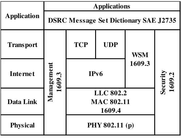
In the U.S., DSRC technologies support wireless communications within a VANET. DSRC-related standards include IEEE Std. 802.11-2012 [5], IEEE Std. 1609/WAVE [6] [7] [8] [9] [10], and SAE J2735 Message Set Dictionary [11]. Figure 2.2 shows the DSRC reference model.

(33)

While the 802.11 family is well-understood, 802.11 unicasting is not well-suited to the VANET environment [23]. The IEEE Std. 802.11 supports safety beacons via broadcast transmissions. Because such broadcasts are unacknowledged, receipt by other nearby vehicles is not guaranteed. Channel availability is performed using Carrier-Sense Multiple Access with Collision Avoidance (CSMA/CA). While sensing of the carrier delays a transmission which would otherwise cause a collision, CSMA/CA does not prevent all such collisions, especially in the hidden node scenario [24] in which one vehicle cannot sense that a transmission would collide with another transmission from a nearby vehicle. When transmitters sense the carrier is busy, they employ a back-off scheme to re-attempt a transmission at a randomly selected future time controlled using the Congestion Window (CW) parameter.

The IEEE 1609/WAVE stack is built on top of the 802.11 MAC and PHY layers and provides further capabilities, such as: channel allocation and multi-channel access, priority queueing and channel routing, congestion control, security and privacy mechanisms, and an application programming interface (API) for messaging. WAVE supports both IPv6-based data transfers and non-IP-based traffic through the WAVE Short Message Protocol (WSMP). IEEE 1609.3 specifies the WAVE Management Entity (WME) and corresponding network services, as well as WSMP. Channel coordination is a collection of enhancements to the IEEE 802.11 MAC, and interacts with the IEEE 802.2 LLC and IEEE 802.11 PHY; IEEE 1609.4

Figure 2.2 DSRC reference model

Transport TCP UDP

Data Link

Physical Application

Applications

DSRC Message Set Dictionary SAE J2735

M a n a g e m e n t 1 6 0 9 .3 WSM 1609.3 S e c u r it y 1 6 0 9 .2 Internet IPv6 LLC 802.2 MAC 802.11 1609.4

(34)

describes multi-channel operations. WAVE security services are specified in IEEE 1609.2. The design of IEEE 1609/WAVE supports a single control channel (CCH) and six service channels (SCH), and it is generally assumed that the CCH will be primarily dedicated to safety applications [12]. Channels are defined in the 5.9 GHz range and typically occupy 10 MHz each, although the potential exists for 5 MHz and/or 20 MHz channels. While the WAVE standard does not preclude multiple channel-dedicated radios for continuous channel access, it also supports three additional options for periodic channel switching, commonly known as alternating, immediate, and extended channel access modes. Sync intervals split the channel at a rate of 10 Hz, which CCH and SCH intervals then typically split equally to support channel switching. A 4ms guard interval separates channel switches, resulting in a CCH interval of (½ x 1/10s) – 4ms = 46ms. Continuous channel access is also supported. Vehicles operate autonomously to synchronize clocks using an external GPS or a WAVE-advertised timing service.

The WAVE standard addresses message priority using four different Access Classes (AC) per (CCH or SCH) channel, AC0 (lowest priority) to AC3 (highest priority), with the MAC layer maintaining separate queues and channel access for each AC [12]. The WAVE contention mechanism is similar to the one used in conventional Wireless Local Area Network (WLAN) and the IEEE 802.11e Enhanced Distributed Channel Access (EDCA) Quality of Service (QoS) enhancements [25]. During packet transmission selection, the four ACs first contend internally with the winning packet then contending for the channel externally using its contention parameters. Each AC specifies a number of Arbitration Inter-Frame Spacing (AIFS) and CW slots and each AC waits at least its AIFS slots, plus additional slots determined by the selected CW value.

Built upon the SAE J2735 DSRC Message Set Dictionary [11], the VANET applications are over the 1609/WAVE stack. Data elements that enable many safety applications are

Table 2.1 DSRC device classes and operating parameters

RSU Class Maximum output power (dBm) Communications zone (meters)

A 0 15

B 10 100

C 20 400

(35)

described in the most important message in the J2935 standard [12], the BSM, which every vehicle broadcasts at a nominal rate of 10 Hz. The BSM is divided into i) Part I mandatory elements such as position, motion, braking status, and vehicle size and ii) Part II optional elements such as vehicle events, path history and path prediction. Additionally, SAE J2735 defines non-safety messages, such as for toll collection, and provides guidelines on message prioritization among different message types. Applications may involve strictly V2V messaging using an On-Board Unit (OBU), or may also involve the use of Roadside Units (RSUs) to support vehicle-to-infrastructure (V2I) communications. The Federal Communications Commission (FCC) defines four classes for DSRC device operations with desired communications zones ranging from 15 to 1000 meters, as shown in Table 2.1 [26] [12]. The most commonly-expected operations category is Class C with a transmitter power of 20 dBm and an expected range of approximately 400m. While vehicles and infrastructure expect to communicate reliably over these ranges, radio-blocking obstacles and other interference that prevent message delivery challenge the safety effectiveness of all applications.

To successfully reduce injuries and fatalities, vehicle safety applications require high penetration rates of DSRC-enabled vehicles that successfully deliver safety information to nearby vehicles with low loss rates. To quickly alert users, safety applications often define performance requirements in terms of metrics such as: BSM transmission rate, Packet Error Rate (PER), IPG, latency (i.e., age of the data in the outgoing BSM [27]), and time to alert (i.e., time from BSM generation until the user is notified).

Devices within 1-300m of a transmission should receive them with a maximum PER of 10%, assuming measurements of the radio transmission pattern are done in an open field with “no man-made or natural structures that would reflect 5.9 GHz radiation within 2.5 kilometers (km) of the test vehicle(s)” [27].

(36)

vehicular density scenarios remains a potential issue that may impact the effectiveness of DSRC and supported safety applications [28].

2.3

Radio Propagation Model (RPM) Literature Review

A radio propagation model (RPM) describes the expected coverage area of a node (e.g., a transmitting vehicle) by characterizing the propagation of radio waves through space, typically as a function of frequency, distance, and/or other parameters. Models typically predict the amount of path loss, or reduction in power density (i.e., attenuation) along the links from the transmitter to each potential receiver. A RPM also often accounts for signal power changes due to the consequences of fading and/or shadowing. Vehicular channel characteristics differ from traditional mobile models in that they are highly dependent upon the existence of LOS paths. Measurement campaigns show that the variety of the types of objects impacts LOS conditions differently, thus making non-line of sight (NLOS) (i.e., LOS blockage from objects) a key factor in modeling V2V propagation channels [29].

Vehicular channel path loss models are based on RPMs and often account for power reductions, or fading, resulting from independent effects often classified as i) large-scale fading, ii) and small-scale fading. Large-scale fading, also called shadow fading, models power losses as varying from one transmitter-receiver link to another, changing slowly as distances between vehicles vary (e.g., over distances that are large compared to a wavelength), depending on the physical environment (e.g., urban, rural, suburban). Large-scale fading models often depict variations as random processes, although some models [30] [31] [13] treat signal fading deterministically based on obstructing obstacles between vehicles. Contrastingly, small-scale fading varies over space in a seemingly random way [32] and changes rapidly, i.e., over travel distances of a wavelength or less, accounting for the results of multi-path fading, power delay profiles, and the Doppler spectrum. Large- and small-scale fading are also sometimes referred to as slow and fast fading, respectively.

(37)

obstacles. The authors of [29] survey VCMs, comparing geodata availability and the usability of models at link or system levels, providing guidelines for the selection of suitable channel models. Models are classified based on their implementation approach (i.e., deterministic (D) or stochastic (S)) and geodata availability (i.e., geometry-based (GB), or non-geometry-based (NG)).

Vehicular scenario differences are sometimes classified and studied in terms of environmental commonality, such as: highway, rural street, suburban neighborhood, urban street, and urban intersection [29] [33]. However, measurements studies are quite rare for specific environments such as: multilevel highways, tunnels, parking garages, bridges, and roundabouts [29]. Additionally, vehicular differences extend beyond the myriad of passenger car shapes, including scooters and public and commercial transportation vehicles, making the propagation characteristics for one vehicle type not readily applicable to other types [29].

The simplest model, often used in VANET simulation, is the unit-disk model, in which vehicles can communicate with each other if they are within a threshold distance and cannot communicate otherwise [34]. The authors of [35] conclude that “a complex shadow fading environment is well approximated by a simpler and more tractable unit-disk model.”

The free space model, also known as the Friis model after its author, models a single, unobstructed communication path [36]. When all V2V links are symmetrical with identical communications limits, then the free space model essentially behaves as the unit disk model.

Another commonly simulated RPM in VANET is the two-ray ground model, which takes into account signal reflection from the road surface and captures additional path loss as in IVC [37]. Because signals between road-based vehicles are assumed present in at least direct LOS and ground reflection, the two-ray ground model seems more appropriate for VANET than the free-space model.

(38)

was characterized by the Weibull distribution. A special case of the general gamma distribution, the Nakagami-m fading model determines signal power reception probabilistically dependent on model parameters that simulate fading levels and may be described as:

; , = _! " $# , 2-1

where is the Nakagami parameter (i.e., shape parameter), Γ is the gamma function, and is the average power of multipath scatter field, which controls the distribution spread.

Stochastic models determine the physical parameters of the vehicular channel in a completely probabilistically way without recognizing fundamental geometry [34]. Stochastic communications modeling could therefore differ dangerously from real behavior, negatively impacting simulations of transmission-critical safety applications [31].

To reduce the randomness of stochastic models, geometry-based deterministic (GBD) models [29] estimate additional path loss using geodata that describes environmental conditions such as the locations of potentially radio wave inhibiting buildings. Examples include CORNER [30] and [31] [13] that deterministically model signal fading in the presence of obstacles that obstruct V2V line of sight (LOS).

To avoid environmental generalities, experiments that capture signal behavior from actual devices operated by typical drivers in realistic environments best serve the need to realistically characterize wireless vehicular channels [29]. However, numerous measurement studies report highly variable and often contradicting results for the same environments in path loss exponents [29] [33] delay spread, and Doppler spread [33], further supporting the thesis that environmental differences significantly prevent an easy characterization of the vehicular channel. For example, crowded highways were found to exhibit large path loss variations [33]. Additionally, the authors of [39] found that the shorter critical distance may be caused by more densely distributed objects like vehicles and pedestrians on the road, creating reflections from points higher than the ground. If measurements for a specific environment are not available, then NG models provide inconsistent results [29].

(39)

lognormally by [34] and using a multiple knife-edge model by [43]. The authors of [44] assert that obstruction by a large building does not involve a pure shadowing but heavily reduces the received power.

A progressive series of models combining distance-based attenuation with building modeling has been proposed by the authors in [42] [45] [46]

The authors of [47] propose a hybrid solution that differentiates between LOS conditions using one set of settings for LOS conditions, and another for Around the Corner (ATC) settings, based on experimental measurements. The authors of [48] propose a similar approach, with different settings for LOS vs. NLOS, using a multi-ray propagation model and including the “foliage” effect in both NLOS and LOS models. Similarly, the authors of [30] classify vehicle communications potential into one of three cases: LOS, NLOS1 (NLOS with one corner along the path) and NLOS2 (NLOS with two corners along the path). The authors of [44] also use two classifications of NLOS, but simulate only in a Manhattan grid scenario.

Because radio waves can physically penetrate one or more buildings, models based on direct LOS alone are insufficient, leading the authors of [31] to collect empirical results showing the outcomes of building shadowing in urban environments. Gathering measurements using IEEE 802.11p devices, the authors of [31] present a realistic, yet computationally inexpensive path loss simulation model that uses the number of obstacle walls and distances intersected between them to estimate the effect that buildings and other obstacles have on the radio communications. However, in later work, the authors of [49] point out that “simulating path loss in (sub)urban environments to capture predictable shadowing effects seems to require more complex models than attenuation per wall or attenuation per meter of penetration approaches” while noting that the computational complexity of the resulting required ray-tracing approaches makes this prohibitive. Similarly, the authors of [30] propose CORNER, “a low computational cost yet accurate urban propagation model for mobile networks” that uses information from urban digital maps to estimate building and obstacle presence along the signal path between two vehicles, classifying the propagation environment between them.

(40)

propagation but remains impractical for evaluating typically large-scale VANETs [47] since it requires site-specific propagation details [34] and does not account for mobile obstacles.

2.4

Vehicular Channel Models

A vehicular channel model (VCM) is an RPM that describes a transmitting vehicle’s expected coverage area. VCM measurement campaigns indicate that variation in signal attenuation arising from the static and dynamic physical world features is strongly correlated over both time and space (i.e., temporally and spatially, respectively) [29]. Thus, the non-stationarity of the channel makes Wide Sense Stationary Uncorrelated Scattering (WSSUS) assumptions non-applicable and most importantly distinguishes the characteristics of V2V channels from the behaviors of conventional cellular networks [33].

2.4.1 Path Loss

Path loss represents the attenuation that results from the propagation of signals originating from a transmitter, ', and is measured as the net change between the transmitter power and the Receiver Signal Strength (RSS) (in dBm), adjusted for antenna gains:

( ) *)+, = (-*)+ , − (/ ) *)+ , + -*)+, + /*)+,, (2-2)

where ( ) is the total path loss in decibels (dB) along ), the distance between the receiver and the transmitter, (_- is the transmitter power (e.g., 20 dBm), (_/ ) is the received power, and _- and _/ are the antenna gain levels in dB of the transmitter and receiver, respectively. 2.4.2 Probability of Packet Reception

We model successful packet reception by considering a receiver sensitivity threshold, (_-1: if the received power, (_/ ) , is larger than (_-1, we assume that the packet is successfully received. PRR is assumed equal to the probability of successfully receiving a signal at the receiver. Ideally, the PRR of short links should be 100% and the PRR of long links should be close to 0%. PRR can be estimated using the link’s projected path loss ((2-2) as:

(22 ) = Pr*(-1 ≤ (/ ) , = Pr*( ) < ( -1,, (2-3) where the path loss threshold, ( _-1 = (_-− (_-1 + _-+ _/.

As Pr*7 ≤ 8, = 9_: 8 , where 9_: 8 is the cumulative distribution function (cdf) of 7, the probabilities in (2-3 may be re written in terms of their cdfs:

(41)

In effect, the probability of packet reception can be derived from the distribution functions that describe path loss:

(22 ) = 9C;A ( ) , (2-5)

where 9C_;A ( ) is the complementary cumulative distribution function (ccdf) of the path loss function.

2.5

Path Loss Models

In this section, we present several widely used path loss models that we will evaluate in Section 5.5 against field operational test data.

2.5.1 Deterministic Path Loss Models 2.5.1.1 Unit Disk Path Loss

Perhaps the simplest conceptual model of path loss is the unit disk path loss model that ignores fading effects altogether and assumes only that those receivers within a limited communications range (i.e., unit) of senders successfully receive signals stronger than the receiver sensitivity threshold (and thus successfully receive packets), while those outside of the range do not. Path loss is given as:

( DE ) = F0, ) ≤ )_{∞ ≥ (} _-1_{, ) > )}H_H , (2-6)

where )_H is the distance that limits reception. Thus, PRR for unit disk path loss is: (22DE ) = Pr*( DE ) ≤ ( -1,

= F1, ) ≤ )_{0, ) > )}H

H .

(2-7)

While failing to accurately reflect waveform propagation effects that are observed in nature, the model is often useful conceptually to address simple node behaviors.

2.5.1.2 Free Space Model

The free space model (i.e., the Friis model), models a single, unblocked communication link where the receiver power, (_/ ) , in ((2-2) deterministically depends only on the transmitted power, antenna gains, and distance between nodes, and is [36]:

(/ ) *L, =(-*L,_4O)- /M , (2-8)

where _- and _/ are the gains of the transmitter and receiver, respectively, and M =P

Q is the

(42)

Assuming for the DSRC environment symmetrically matched antennas (i.e., setting _S, and to 1), converting between Watts and dBm by (*L, = 10 T*UV ,W /1000, and substituting ((2-8) into ((2-2), we can rewrite free space path loss (FSPL) in dB as:

( YZ;A ) *)+, = 20\]^_`a4O)_{M b.} (2-9)

When the communications parameters in the vehicular environment in ((2-8) are homogenous with symmetrically limited communications distances, (i.e., some value of )_H in ((2-6) applies to ) in ((2-9)), then the free space model essentially becomes the unit disk model.

2.5.2 Probabilistic Path Loss Models 2.5.2.1 Lognormal Path Loss

A large-scale fading model commonly used to model the vehicular channel [39] [29] is the lognormal path loss model that relies on two key parameters to model path loss:

i) c, the path loss exponent that accounts for average large-scale variations as a function of distance and

ii) ii) d, the standard deviation of the scatter of received power about the average that reflects minor variations that follow a zero mean normal distribution (i.e., 7e~g 0, d ).

Thus, received signal strengths at locations equally distant from the transmitter are considered i.i.d. random variables, with lognormal path loss as:

( A ) *)+, = ( )` + 10c\]^_`a₎)

`b + 7e, (2-10)

where ( )_` is the path loss at the reference distance )_` (e.g., typically < 10m), ) is the distance between sender and receiver, c is the path loss exponent, and 7_emodels the path loss variation across all locations at distance ).

(43)

(22A ) = Pr*( A ) ≤ ( -1,

= Pr h( )` + 10c\]^_`a₎)

`b + 7e ≤ ( -1i

= Pr h10c\]^_`a₎)

`b + 7e ≤ ( Ei,

(2-11)

where ( _E = ( _-1 − ( )_` is a simplifying constant.

Considering the distribution of 7_e, ((2-11) can be expressed as [39]: (22A ) =_√2Od1 k exp o− 2d p)

q r,s

t

= 1_{2 +}1_{2 erf o}v ), c √2d p,

(2-12)

where the error function is erf 8 =

√wx " S y

z ) ,v ), c = 10c\]^_`{r|}r ~, and )H is the

limiting distance at which (_/ ) ≥ (_-1 (i.e., equivalently, ( ) ≤ ( _-1) in the absence of small-scale fading (d = 0), i.e., )_H = 10T•€W•_.

2.5.2.2 Dual-slope Distance-breakpoint Path Loss Model

(44)

( ƒ; ) = ( )` +

„ …

†10c_\]^_`a₎)

`b + 7e , )` ≤ ) ≤ )‚

10c_\]^_`a)₎‚

`b + 10c \]^_`a

)

)‚b + 7e , ) > )‚

, (2-13)

In conventional direct LOS models, )_‚ is the Fresnel distance to the point where the first Fresnel zone touches the ground, which can be calculated as )_‚= ‡ˆ<ˆ‰

Š , where ℎ- and ℎ/ are

antenna heights of the transmitter and receiver, respectively, and M is the wavelength [39]. For example, when the height of the transceiver antennas on the vehicles are ℎ_- = ℎ_/Œ = 1.5m and the wavelength M ≈ 0.0508m, then )_‚ ≈ 177m in the vehicular environment. However, for our model analysis, we allow )_‚ to be adjustable.

PRR can be estimated for the dual-slope distance breakpoint model by considering each case in ((2-13) separately. Turning first to the case that )_` ≤ ) ≤ )_‚, the packet receipt likelihood is [50]:

(22ƒ; ) = *( ƒ; ) ≤ ( -1,, )` ≤ ) ≤ )‚

= Pr h10c_\]^_`a₎)

`b + 7e ≤ ( Ei

=1_{2 +}1_{2 erf o}v_ ), c_ √2d_ p.

(2-14)

where v_{_} ), c_{_} = 10c_{_}\]^_{_`}{r

r~, )_ = 10 T•€

W• _.

Similarly, when ) > )_‚, then PRR in this case is [50]: (22ƒ; ) = Pr*( ) ≤ ( -1,, ) > )‚

= Pr h _+ 10c \]^_`a₎)

‚b + 7e ≤ ( Ei

= 1_{2 +}1_{2 erf o}v ), c √2d p.

(2-15)

where v ), c = 10c \]^_{_`}{r’_rr ~, ) = 10

T•€ “

W• _{, and} _{_} = 10c_{_}\]^_{_`} )_‚ _.

2.5.2.3 Nakagami-m Small-scale Fading

(45)

varies with distance, providing insight into environmental changes in the fading channel. For example, in [52], indicates a change from Rician fading ( > 1) at shorter distances with stronger LOS possibilities to Rayleigh fading ( = 1) as distance increases and d