Spatial Profiles in the Singular Solutions of the 3D Euler Equations and Simplified Models

(1)

Equations and Simplified Models

Thesis by

Pengfei Liu

In Partial Fulfillment of the Requirements for the degree of

Doctor of Philosophy

CALIFORNIA INSTITUTE OF TECHNOLOGY Pasadena, California

2017

(2)

(3)

ACKNOWLEDGEMENTS

I would like to extend my deepest gratitude to my thesis adviser, Prof. Thomas Yizhao Hou, for his continuous support, guidance and encouragement. Prof. Hou introduced me to the field of mathematical fluid mechanics, and I have truly enjoyed my research in this fascinating area. Prof. Hou dedicates to work on hard and impactful research problems, which deeply influenced me and shaped my view of scientific research. I benefited tremendously from his deep mathematical insight and broad vision of science. Moreover, Prof. Hou also gives me a lot of help in my personal life, and I could not have imagined having a better mentor.

I also want to thank Profs. Oscar Bruno, Dan Meiron and Houman Owhadi for kindly serving in my thesis committee. I took Prof. Bruno’s courses on PDE, and what I learned in that class prepared me for my research on fluid equations. I got several opportunities to talk with Prof. Owhadi on multi-scale analysis and uncertainty quantification, and benefited a lot from his expertise.

I feel honored to have had some stimulating discussions with many brilliant math-ematicians, especially Prof. Tianling Jin from HKUST, Prof. Zhiwen Zhang from HKU, Prof. Yao Yao from GaTech, Prof. Kiselev from Rice University, Prof. Qin Li and Dr. Xiaoqian Xu from University of Wisconsin, Mr. Pengchuan Zhang and Dr. Maolin Ci from Caltech, and more. Their knowledge truly inspired me.

The Computing+Mathematical Sciences department at Caltech provides an extremely cozy environment for studying and research. I want to thank the CMS staff mem-bers, especially Carmen Sirois and Sydney Garstang, for their help.

I have been fortunate enough to make some very good friends, and without their help I would have never reached this point. I would like to thank their accompany and support, especially Ting Jiang, Chengdi Lai, Yong Huang, Yilin Mo, Niangjun Chen, Lingwen Gan, Qiong Zhang, Duo Han, Xiaoqi Ren, and more.

(4)

ABSTRACT

The partial differential equations (PDE) governing the motions of incompressible ideal fluid in three dimensional (3D) space are among the most fundamental non-linear PDEs in nature and have found a lot of important applications. Due to the presence of super-critical non-linearity, the fundamental question of global well-posedness still remains open and is generally viewed as one of the most outstanding open questions in mathematics. In this thesis, we investigate the potential finite-time singularity formation of the 3D Euler equations and simplified models by studying the self-similar spatial profiles in the potentially singular solutions. In the first part, we study the self-similar singularity of two 1D models, the CKY model and the HL model, which approximate the dynamics of the 3D axisymmtric Euler equations on the solid boundary of a cylindrical domain. The two models are both numerically observed to develop self-similar singularity. We prove the exis-tence of a discrete family of self-similar profiles for the CKY model, using a com-bination of analysis and computer-aided verification. Then we employ a dynamic rescaling formulation to numerically study the evolution of the spatial profiles for the two 1D models, and demonstrate the stability of the self-similar singularity. We also study a singularity scenario for the HL model with multi-scale feature.

(5)

(6)

LIST OF ILLUSTRATIONS

Number Page

2.1 Vorticity and velocity fields in the numerical computation [58]. . . . 13

2.2 Dependence ofG(cl) oncl fors =2. . . 39

2.3 Self-similar profiles ofW fors =2,3,4,5. . . 40

2.4 The self-similar profiles obtained from (2.4.14) and (2.2.4). . . 47

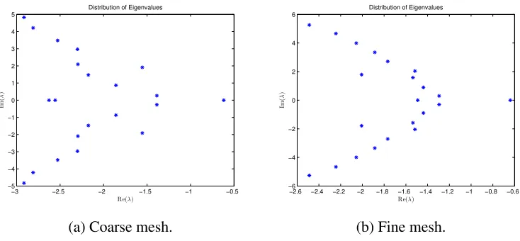
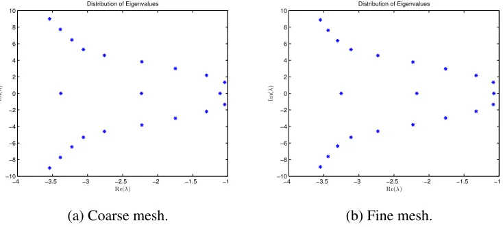
2.5 Leading eigenvalues of the Jacobian matrix (2.4.29). . . 48

2.6 The rescaled solutionsW at different time steps close to singularity. . 52

2.7 The line fitting to determinecw and the singularity timeT. . . 53

2.8 The line fitting to determinecl. . . 53

2.9 The configuration of wwith respect tosatt = 0.0374. . . 54

2.10 The self-similar profiles obtained from (2.4.14) and [40]. . . 56

2.11 Leading eigenvalues of the Jacobian matrix. . . 57

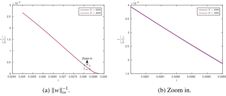
2.12 Blowup rate of kwk∞for the HL model with s= 4. . . 59

2.13 Decay rate ofCl(t) for the HL model withs= 4. . . 60

2.14 Profiles of W and Θ obtained by normalizing their leading order derivatives at the origin. . . 60

2.15 Profiles of W and Θ obtained by normalizing the position where kWk∞ is attained, and the value ofΘ. . . 61

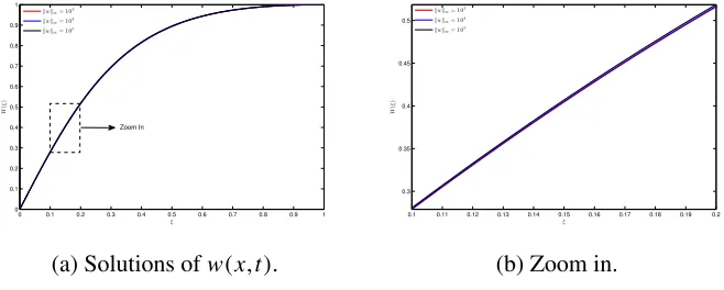
2.16 Evolution of solutions to the dynamic rescaling equations. . . 62

2.17 Evolution of solutions to the dynamic rescaling equations with the second normalization condition. . . 63

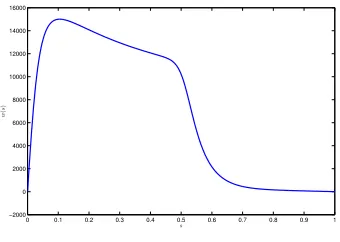
2.18 Growth of the dynamic rescaling solutions with time. . . 63

3.1 Configuration of the potentially singular solutions. . . 67

3.2 Contour plot ofwat the steady state. . . 89

3.3 Linearized stability of the self-similar profiles fors =2. . . 89

3.4 Blow up rate for the solutions of the Boussinesq system withs =4. . 91

3.5 Spatial profiles of the Boussinesq system fors =4. . . 92

3.6 Evolution of the solutions to the dynamic rescaling equations. . . 94

3.7 Evolution of the solutions to the dynamic rescaling equations. . . 94

3.8 Steady state of the discretized dynamic rescaling equations. . . 95

3.9 Finite-time singularity with multi-scale feature. . . 96

(8)

(9)

LIST OF TABLES

Number Page

(10)

C h a p t e r 1

INTRODUCTION

1.1 The Regularity Problem for the 3D Euler and Navier-Stokes Equations

The grand open question

The study of fluid has a long history, and dates back to the works of Leonardo Da Vinci, who made an attempt at studying turbulence, Isaac Newton, who derived the formula for drag force, and Jean le Rond d‘Alembert, who is famous for his paradox that drag force is zero in ideal fluid. The classical equations of fluid dynamics are among the most fundamental partial differential equations, which have found a lot of important applications but are still far from being fully understood.

The 3D incompressible Euler (inviscid) and Navier-Stokes (viscous) equations are the governing equations for the motions of incompressible ideal fluid in 3D space, and take the following simple form,

ut+u· ∇u= −∇p+ν∆u, (1.1.1a)

∇ ·u= 0, (1.1.1b)

where

u(x,t) : R3×[0,T) → R3 describes the velocity field of the fluid, and

p(x,t) : R3×[0,T) → R is the pressure field in the fluid. The diffusion term

ν∆u

models the viscosity, and is derived from the Stokes’ stress constitutive equation

∇ ·τ, τ = 2νε,

where

ε= 1

2(∇u+∇u T_).

(11)

Equation (1.1.1a) is Newton’s second law of motion applied to fluid. The diver-gence free condition (1.1.1b) guarantees the incompressibility of the fluid.

Note that we do not have an evolution equation for the pressure field p(x,t) in (1.1.1). The pressure p(x,t) can indeed be viewed as a Lagrange multiplier, and recovered based on the divergence free constraint (1.1.1b). Taking the divergence of equation (1.1.1a), one can get the following representation for the pressurep(x,t),

p(x,t)= (−∆)−1∂i∂juiuj. (1.1.2)

Equations (1.1.1) can also be written as

ut = B(u,u)+ν∆u, (1.1.3)

where the nonlinear termB(u,u) is defined as

B(u,u) =−u· ∇u− ∇p= P(−u· ∇u). (1.1.4) HerePis the Leray projection operator onto divergence-free vector field,

Pui =ui−∆−1∂i∂juj.

The Euler equations enjoy the following scaling invariant property u(x,t) → λ

And for the Navier-Stokes equations, we have the following scaling-invariance, u(x,t) → τ−1/2u

Note that the scaling transformations determine the two-parameter symmetry group in (1.1.5) for the Euler equations, and the introduction of viscosity ν > 0 restricts this symmetry group to the one-parameter group given in (1.1.6) for Navier-Stokes. Smooth solutions to (1.1.1) conserve the kinetic energy kuk_L2₍_R3₎, and we have

The local posedness of the Euler and Navier-Stokes equations (1.1.1) is well-known. To be specific, given smooth initial data

(12)

with rapid decay at infinity, for example,

|∂_xαu(x,0)| ≤CαK(1+ |x|)−K onR3, for anyα,K,

one has a time interval [0,T), on which unique solutionsu(x,t) exist and satisfy, u(x,t) ∈C∞(R3×[0,T)), ku(x,t)k_L2₍_R3₎ ≤ ku(x,0)k_L2₍_R3₎. (1.1.8)

The classical results regarding the local-wellposedness for the 3D Euler and Navier-Stokes equations are covered very well in the book [59].

However, the question of global well-posedness of the 3D Euler and Navier-Stokes equations (1.1.1) remains open. Namely, it is not known whether the existence time-interval [0,T) in (1.1.8), on which the solutions are unique and remain smooth, can be extended to [0,+∞) or not. The global well-posedness of the 3D Navier-Stokes equations (ν > 0) is generally viewed as one of the most important open problems in mathematics, and listed in the millennium problems by the Clay Institute1. The major difficulty for the global regularity of the 3D Navier-Stokes equations lies in the supercritical nature of the nonlinearity, see [74]. To be specific, thea priori estimate (1.1.7) of the solutions, namely, kuk_L2₍_R3₎, gets worse when we zoom in

the solutions according to the invariant scaling of the equations (1.1.6),

kτ−1/2u

x

τ1/2,

t τ

k_L2₍_R3₎ > ku

x, t τ

k_L2₍_R3₎, for τ > 1.

In another word, with only thea prioriestimate (1.1.7), one cannot use the diffusion termν∆uto control the nonlinear termB(u,u) based on scaling argument.

The potential finite-time singularity of the 3D Euler and Navier-Stokes equations (1.1.1) can be more clear when written in the vorticity form,

ωt+u· ∇ω= ω· ∇u+ν∆ω, (1.1.9a)

u= ∇ ×∆−1ω, (1.1.9b)

where the vorticityω is the curl of the velocity,ω(x,t) =∇ ×u(x,t).

The first term on the RHS of (1.1.9a) is called the vortex stretching term, which is absent in the 2D setting. Note that∇uis of the same order asω, and thus the vortex stretching term has a formal quadratic scaling with respect to the vorticityω, and can lead to potential formation of a finite-time singularity forω.

(13)

For the 3D Euler equations (1.1.1), namely the case that ν = 0, due to the lack of regularizing mechanism (viscosity), even the local well-posedness of equations can only be obtained with regular enough initial data [44].

See the surveys [31, 17] for more background about this outstanding open question.

Partial Results Concerning the Regularity of Euler and Navier-Stokes

A lot of effort has been devoted to the regularity problem of Euler and Navier-Stokes equations, and we list a few of these results below.

For smooth enough initial data, the Euler and Navier-Stokes equations in the 2D set-ting are globally well-posed. This is because in the 2D setset-ting, the vortex stretching term in (1.1.9) vanishes, and one can geta priori global estimate for the maximal vorticity kωk_L∞. Then the global regularity of the solutions follows.

For the 3D Euler equations, the celebrated Beale-Kato-Majda (BKM) criterion [6, 26] asserts that the solutions develop finite-time singularity at timeT if and only if

Z T

0

kω(·,t)k_L∞dt = +∞. (1.1.10)

The BKM criterion imposes certain constraint on the blow up rate of the maximal vorticity. For example, kωk∞cannot blow up as (T−t)β with some β >−1. The non-blowup criterion of Constantin, Fefferman and Majda [18] focuses on the geometric aspects of 3D Euler flows instead and asserts that there can be no blowup if the velocity fielduis uniformly bounded and the vorticity directionξ =ω/|ω|is sufficiently “well-behaved” near the point of maximum vorticity.

The theorem of Deng, Hou and Yu [19, 20] for the 3D Euler equations is similar in spirit to the Constantin-Fefferman-Majda criterion, but confines the analysis to localized vortex line segments. They assert that if the vorticity direction is “well-behave” on a local region near maximum vorticity, then the solutions remain regu-lar. To be specific, their theorems allow the area of the region converges to zero. For the 3D Navier-Stokes equations, if the initial data is small enough in certain critical norm, namely invariant under the scaling (1.1.6), say

kuk_L2k∇uk_L2,

(14)

The criterion of Prodi [67] and Serrin [71] claims that for 2

p+ 3

q =1, 3< q ≤ +∞, (1.1.11) if

ku(x,t)k_Lp₍_Lq₍_R3₎_,_[0_,_T₎₎ < +∞,

then the solutions can be extended smoothly beyond timeT, where

ku(x,t)k_Lp₍_Lq₍_R3₎_,_[0_,_T₎₎ = (

Z T

0

ku(x,t)kp

Lq₍_R3₎)

1/p_.

The condition with p = +∞, q = 3 in (1.1.11) also implies regularity but is essen-tially different from (1.1.11). It is proved in [24] by Escauriaza, Seregin and Sverak, which relies on a unique continuation property for backwards heat equations. Important progress has been made in understanding weak solutions of the Navier-Stokes equations, namely solutions satisfy (1.1.1) in distribution. Leray [55] showed the existence of weak solution with suitable growth properties, while the uniqueness of weak solutions for Navier-Stokes equations is still unknown.

Scheffer [69] proved a partial regularity theorem for suitable weak solutions of the Navier-Stokes equations. Caffarelli-Kohn-Nirenberg [9] improved Scheffer’s re-sults, and Lin [57] simplified the proofs of the results in Caffarelli-Kohn-Nirenberg. The partial regularity result asserts that for suitable weak solution of the Navier-Stokes equations, the one-dimensional Hausdorff measure of the singular set has to vanish. In the case of Navier-Stokes equations with axial symmetry, this result implies that singularity can only take place on the symmetric axis.

Due to the lack of analytical tools for super-critical nonlinearity, major break-through in analysis is needed to resolve this open problem. T. Tao [73] formalized this super-critical barrier by proposing a 3D model, where the nonlinearity term B(u,u) in (1.1.4) is replaced by an averaging term ˜B(u,u), and one gets

(15)

Numerical Search of Potential Finite-time Singularity

Besides the analytical results mentioned in the previous subsection, there also exists a sizable literature focusing on the numerical search of a finite-time singularity for the 3D Euler equations. These numerical computations have led to improved understanding about the vortex stretching or depletion of nonlinearity.

Representative work in this direction includes the result by Grauer and Sideris [33], and the result by Pumir and Siggia [68] on the 3D axisymmetric Euler equations. Finite-time singularity was reported in those numerical computations. However, by exploiting the analogy between 3D axisymmetric Euler equations and 2D Boussi-nesq system, E and Shu [22] studied the potential development of finite-time sin-gularity for the 2D Boussinesq system with higher resolution and initial data com-pletely similar to those in [33, 68]. No finite-time singularity was observed, indi-cating that the finite singularity reported in [33, 68] was likely numerical artifact. Kerr and his collaborators [47] studied Euler flows generated by a pair of perturbed anti-parallel vortex tubes, and a finite-time singularity was reported. Hou and Li [39] repeated the computation in [47] with higher resolutions to reproduce the sin-gularity scenario, and no finite-time sinsin-gularity was observed. By using newly de-veloped analytic tools based on rescaled vorticity moments, Kerr also confirmed in [46] that the solutions computed from initial data in [47] eventually converge to superexponential growth and are unlikely to lead to a finite-time singularity. Other interesting pieces of work are [10, 72], which studied axisymmetric Euler flows with complex initial data and reported singularities in the complex plane. In [8], the Navier-Stokes equations were numerically solved using Kida’s high-symmetry initial data, where rapid growth of the solution was observed, but no conclusion could be made regarding singularity formation in finite time.

(16)

1.2 The Role of Self-similarity in Nonlinear PDEs

Self-similar Singularities

Self-similarity plays an important role in the singularity formation of nonlinear PDEs. Consider the following nonlinear evolution PDE

ut = N(u), (1.2.1)

whereN(·) is a nonlinear term. Assume that the solution to (1.2.1) develops finite-time singularity at a single space finite-time point (x,t) = (x0,t0). We shift the singularity

point to the origin, and denote x0andt0as shifted variables x0= x−x0, t0=t−t0.

Then if the local solution of (1.2.1) develops asymptotic structure u(x,t)≈ (t0)cu_U₍ x

0

(t0₎cl), (1.2.2)

with somecu andcl, we say the solution develops self-similar singularity. Scaling invariant property of the equation is necessary for self-similar singularity.

Self-similar singularities arise in a lot of nonlinear PDEs governing natural phe-nomenon. A finite time singularity signals certain physical events such as the solu-tions change topology, or the emergence of a new structure. Self-similar singularity reveals the universal law and scaling in the corresponding process.

Examples of self-similar singularities arise in free surface flows [76, 75, 7], reaction diffusion equations [32, 35, 63, 29], nonlinear Schödinger equations [21, 65, 62, 61, 27, 60, 51, 54, 52, 64]. See [23] for a survey of self-similar singularity.

Plugging the self-similar ansatz (1.2.2) into equation (1.2.1), if the scaling of the nonlinear terms match each other, we can get the following self-similar equation governing the self-similar profileU(ξ) in the ansatz (1.2.2),

clξ· ∇U(ξ) = N(U(ξ))+cuU(ξ). (1.2.3)

(17)

for a continuous set of scaling exponentscu,cl. These local solutions are in general inconsistent with the boundary or initial conditions of the nonlinear PDE (1.2.1), and imposing these boundary conditions leads to a nonlinear eigenvalue problem, whose solution yields irrational scaling exponents in general.

Major Difficulties for Second Kind Self-similar Singularities

We study the self-similar singularity of the Euler equations and related models in this thesis. Plugging the ansatz (1.2.2) into the Euler equations (1.1.1) with ν = 0, and matching the scaling of nonlinear terms, one can get the following condition

cu= cl−1,

and the exponent cl cannot be determined by a simple dimensional analysis. Thus the singularity scenarios that we investigated are of the second kind.

Since the self-similar ansatz approximates the singular solutions locally on a region close to the singular point, the self-similar profiles do not necessarily have finite energy, even though the solutions to the Euler equations enjoy energy conservation. For the Euler singularity scenario that we consider in this thesis, the self-similar profilesU are actually increasing with a fractional power at infinity, which makes it hard to find an appropriate function space to study the self-similar profiles. For the 3D axisymmetric Euler equations that we consider in this thesis, the so-lutions do not enjoy a perfect scaling invariance centered at the singularity point on the solid boundary, and in deriving the self-similar equations (1.2.3), one needs to discard some lower order terms. In this case one needs certain stability of the self-similar profiles to justify the neglecting of low order terms.

Besides the nonlinear terms in the self-similar equations, the equations are also non-local in nature, since to recover the pressure field in (1.1.2), one needs the velocity field on the whole domain to invert the Laplace operator. The non-locality makes solving the self-similar equations even more challenging.

(18)

1.3 Summary of the Thesis

Self-similar Singularity of 1D Models of the 3D Axisymmetric Euler Equations

We first consider two 1D models approximating the dynamics of the 3D axisymmet-ric Euler equations on the solid boundary of a periodic cylinder, the CKY model, and the HL model. The HL model is motivated by the recent finite-time singular-ity scenario reported by Hou and Luo, and the CKY model is derived as a further approximation of the HL model by simplifying the Biot-Savart law.

For the CKY model, we proved that there exists a discrete family of analytic self-similar profiles corresponding to different leading orders of the profiles at the origin. In the proof, we first construct local self-similar profiles using the power series method, and then extend the local profiles to infinity by solving a nonlinear ODE system. We use computer-aided verification technique to prove the existence of cl that makes the profiles satisfy the required decay condition at infinity. Some asymptotic properties of the self-similar profiles at infinity are also proved.

Then we use the dynamic rescaling formulation to study the self-similar profiles of the two 1D models numerically. In the dynamic rescaling formulation, scaling terms are added to the equations based on the scaling-variant properties of the solu-tions, and the resecaling equations govern the evolution of the spatial profiles of the singular solutions. We use the dynamic rescaling formulation to demonstrate the stability of the self-similar singularity. To be specific, starting from initial data suf-ficiently close to the self-similar profiles, the solutions will also develop singularity with the same asymptotic structure as the self-similar ansatz.

For the HL model, we also show that the solutions can develop singularity at mul-tiple scales for certain initial data, which is different from the CKY model.

Two Types of Singular Behaviors for the 3D Axisymmetric Euler Equations

The 3D Euler axisymmetric equations away from the axis are qualitatively similar to the 2D Boussinesq system. In the finite-time singularity scenario reported by Luo and Hou [58], the leading order terms in the 3D axisymmetric Euler equations are exactly the same as the 2D Boussinesq system, and we use the dynamic rescal-ing formulation for the 2D Boussinesq system to study the self-similar srescal-ingularity reported in [58]. The dynamic rescaling equations of the 3D axisymmetric Euler equations can be viewed as a perturbation to that of the 2D Boussinesq system with the perturbation term converging to zero exponentially fast in time.

(19)

family of local self-similar profiles for the 2D Boussinesq system. The proof needs a modification of the Cauchy-Kowalevski majorization argument [50] due to the existence of a formal singularity of the self-similar equations at the origin.

We consider two types of initial data with different leading order properties. The first initial data correspond to the singular solutions reported by Luo and Hou, where self-similar singularity is observed. Our numerical study suggests that the 2D Boussinesq system develops stable self-similar singularity, and the stability of profiles confirms the singularity for 3D axisymmetric Euler reported in [58]. For our second choice of initial data for the dynamic rescaling equations, the so-lutions develop a singularity themselves. In another word, there is a smaller scale generated, and correspondingly the solutions of the original Euler equations develop finite-time singularity at multiple scales, which is very different from the behavior of the singular solutions reported by Luo and Hou in [58]. This result agrees with our direct numerical simulation of the 2D Boussinesq system.

The stability studies for the self-similar profiles may help to get better understand-ing about the sunderstand-ingularity formation mechanism for the 3D Euler equations.

A Family of 3D Models of the 3D Axisymmetric Euler Equations

For the axisymmetric Euler and Navier-Stokes equations written in cylindrical coor-dinates, Hou and Lei [37] removed the convection terms and obtained a 3D model of the Euler and Navier-Stokes equations. This model enjoys a similar energy identity and shares several non-blowup criteria with the 3D Euler and Navier-Stokes equa-tions [37]. The partial regularity result for the Navier-Stokes equaequa-tions also holds for this new viscous 3D model [36]. Moreover, the inviscid 3D model can develop finite-time singularity under certain Dirichlet-Robin boundary conditions [43]. The numerically observed finite-time singularity will be destroyed if the convection is added back, which reveals the stabilizing effect of convection.

(20)

(21)

C h a p t e r 2

SELF-SIMILAR SINGULARITY OF TWO 1D MODELS

In this chapter, we consider two 1D models of the 3D axisymmetric Euler equations, and investigate the stability of the spatial profiles in their singular solutions.

2.1 Derivation of the Two 1D Models

The two 1D models are motivated by the recent numerical computation of Luo and Hou in [58], and they approximate the dynamics of the axisymmetric Euler equations on the solid boundary of a cylindrical domain.

Leter,eθ andez be the standard vectors defining the cylindrical coordinate system, er = (x1

r , x2

r ,0) T_,

eθ = (x2 r ,−

x1

r ,0) T_,

ez = (0,0,1)T, wherer =

q

x2₁+x2₂. Then the velocity field is called axisymmetric if u= ur(r,x3,t)er +uθ(r,x3,t)eθ +uz(r,x3,t)ez,

namely,ur,uθ anduz do not depend on theθ coordinate. The axisymmatric Euler equations can be written in cylindrical coordinates withz = x3as

utθ+u r

uθr +u z

uθz = − 1 ru

r

uθ, (2.1.1a)

ω_tθ+urω_rθ+uzωθ_z = 2 ru

θ

uθ_z + 1 ru

r_ωθ_,

(2.1.1b)

−[∆− 1

r2]φ

θ ₌ _ωθ_, _(2.1.1c)

where the radial and angular velocity fieldsur anduθare recovered as ur =−∂zφθ, uz =r−1∂r(rφθ).

Note that equations (2.1.1) have a formal singularity at the axisr = 0 due to the 1_r terms, and it can be removed by introducing the transformed variables

u1=uθ/r, w1= wθ/r, φ1= φθ/r. (2.1.2)

One can get the equations foru1andω1as the following,

u1,t+uru1,r +uzu1,z =2u1φ1,z, (2.1.3a)

w1,t+urw1,r +uzw1,z = (u2₁)z, (2.1.3b)

(22)

with Boit-Savart law

ur =−rφ1,z, uz = 2φ1+rφ1,r. (2.1.3d) In the numerical computation [58], (2.1.3) were numerically solved in a periodic cylinder (r,z) ∈[0,1]×S1. It is reported that with initial data

w1(r,z,0) =0, u1(r,z,0) = 100e−30(1−r

2₎4

sin(2πz),

the numerical solutions to (2.1.3) develop finite-time singularity on the boundary (r,z) = (1,0). The vorticity and velocity fields of the potentially singular solutions roughly take the configuration illustrated in Figure 2.1.

The no-flow boundary condition and the symmetry of the data in the axial direction create a compressing flow along the solid boundary of the cylinder, which seems responsible for the numerically observed finite-time singularity.

z

symmetry plane (x,y,0) periodic in z

no flow boundary conditionu·n= 0

ω1>0

ω1<0

u

(a) In the 3D space.

r z

ω1>0

ω1<0

Potential finite-time singularity

u

(b) In the meridian plane.

Figure 2.1: Vorticity and velocity fields in the numerical computation [58].

Motivated by this new finite-time singularity formation scenario in Figure 2.1, Kise-leve and Sverak in [48] constructed an example of 2D Euler solutions in a similar setting, and proved that the maximal gradient of the vorticity field in that example exhibits double exponential growth in time, which is known as the fastest possible rate of growth for the 2D Euler equations. This example provides further evidence that this new finite-time singularity formation scenario reported in [58] is an inter-esting candidate to investigate the potential 3D Euler singularity.

Because of the no-flow boundary condition, we haveur =0,φ1,z =0 on the bound-aryr = 1. Restricting equations (2.1.3) onr = 1 gives the following 1D system,

(23)

whereu(x,t)w(x,t) andθ(x,t) correspond touz,w1andu2₁in (2.1.3).

The 1D model system (2.1.4) is exact in the sense that it is obtained as the restric-tion of the 3D axisymmetric Euler equarestric-tions on the solid boundary without any approximation. To close the above 1D system (2.1.4), one needs an appropriate Biot-Savart law connecting the velocity fieldu(x,t) with the vorticity fieldw(x,t). In [41], Hou and Luo proposed and investigated the following model,

ux = Hw, x ∈[−1,1], (2.1.5a) whereH is the periodic Hilbert transform. Namely,

ux(x)= P.V.1 For odd vorticity fieldw, we can derive by direct integration that

uHL(x) =

We refer to the above model (2.1.5) together with (2.1.4) as the HL-model. The HL-model preserves the odd and even properties of w1 anduz in the axisymmet-ric Euler equations (2.1.3), and can be derived by assuming that the vorticity w1

in (2.1.3) is constant in ther direction near the boundary, see [41, 15]. The finite-time singularity of the HL-model from smooth initial data is proved in [15].

In [14], Choi, Kiselev and Yao proposed the following model,

uCKY(x) =−x

to close the system (2.1.4). We refer to model (2.1.6) together with (2.1.4) as the CKY-model, whose finite time singularity is proved in [14]. The CKY-model is proposed as a further simplification of the HL-model. One can show that the CKY-model is a leading order approximation to the HL-CKY-model at the origin,

uHL(x)−

π

2uCKY(x) =O(x

2_),

x →0.

(24)

The mechanism of the finite-time singularity for the two 1D models is the follow-ing: the positive w(x,t) near the origin creates a compressing flow u(x,t) < 0 according to the Biot-Savart laws (2.1.5), (2.1.6); this compressing flow produces a largerθx(x,t) near the origin according to equation (2.1.4b), since θ(x,t) is con-vected by the velocity field u(x,t); according to equation (2.1.4a), θx(x,t) is the time derivative of w along characteristics, and thus w(x,t) will in turn get larger; this nonlinear amplification mechanism finally leads to finite-time singularity.

2.2 The Self-similar Equations Governing the Self-similar Profiles

One can easily verify that the 1D models (2.1.5) and (2.1.6) both enjoy the following scaling invariant property forλ >0, µ >0,

w(x,t)→ 1 The singular solutions to the two models both develop local self-similar structure around the origin, so we make the following ansatz to the local solutions,

θ(x,t)= (T −t)cθΘ x

Plugging the ansatz into equations (2.1.4), (2.1.5) and (2.1.6), and matching the exponents of (T−t), we get the following relation of the scaling exponents,

cw = −1, cu= cl−1, cθ =cl−2. (2.2.3)

The self-similar profilesU(ξ),W(ξ),Θ(ξ) satisfy the following equations, which are defined onξ ∈ R+ and will be referred to as the self-similar equations,

W(ξ)+clξW0(ξ)+U(ξ)W0(ξ)−Θ0(ξ) =0, (2.2.4a) (2−cl)Θ(ξ)+clξΘ0(ξ)+U(ξ)Θ0(ξ) =0. (2.2.4b) The Biot-Savart laws of the HL-model (2.1.5) and the CKY-model (2.1.6) become

(25)

Note that kθkL∞ is conserved for the two 1D models, and thus we require that

cθ = cl−2≥ 0.

The singularity of the two models are both point singularity, namely, w(x,t) and θ(x,t) remain bounded away from the origin up to the singularity time. This re-quires us to impose the following decay condition at infinity,

Θ(ξ)=O(ξ1−2/cl), _W(ξ₎=_O(ξ−1/cl), _U(ξ) =O(ξ1−1/cl), ξ _→+_∞. _(2.2.6)

The self-similar equations (2.2.4) enjoy the following scaling-invariant property, W(ξ)→W(ξ

λ), Θ(ξ) → λΘ( ξ

λ), U(ξ) → λU( ξ

λ). (2.2.7) The self-similar singularity for the two 1D models are of the second kind, since the scaling exponent cl cannot be determined from dimensional analysis. And to solve the self-similar equations (2.2.4), one needs to find cl such that (2.2.4) have non-trivial solutions, which is essentially a nonlinear eigenvalue problem.

2.3 Existence of Self-similar Profiles for the CKY Model

In this section, we prove the existence of a family of self-similar profiles for the CKY model. The Biot-Savart law of the CKY model

U(ξ)= −ξ Z +∞

ξ

W(η) η dη

can be rewritten as a local relation (2.3.1a) with a global constraint (2.3.1b), U(ξ)

ξ

!0

= W_ξ(ξ), (2.3.1a)

lim

ξ→+∞ U(ξ)

ξ =0. (2.3.1b)

(26)

system. Then we prove that the decay condition (2.3.1b) determines the scaling exponents, and there exists a discrete family ofcl, corresponding to different lead-ing orders ofΘ(ξ), such that the decay condition (2.3.1b) holds for the self-similar profiles that we construct. We prove this part with the assistance of numerical com-putation and rigorous error control. With the decay condition (2.3.1b), we further analyze the far-field properties of these self-similar profiles and prove that the pro-files satisfy condition (2.2.6) atξ = +∞. We have the following theorem.

Theorem 2.3.1. There exist a discrete family of scaling exponent cl and analytic

solutions to the self-similar equations (2.2.4), corresponding to different leading orders of the self-similar profileΘ(ξ)at the originξ =0,

s= min{k ∈ N+| d

k

dξkΘ(0), 0}. (2.3.2) And in the far-field, W(ξ), U(ξ)ξ−1, Θ(ξ)ξ−1 are analytic with respect to a trans-formed variableζ = ξ−1/cl _atζ =_0.

Remark2.3.1. The self-similar profiles that we construct are non-conventional since the velocityU(ξ) does not decay to zero at infinity but grows as

U(ξ) =O(ξ

cl−1

cl ), ξ _→ +_∞.

Correspondingly, the velocity field at the singularity time is Hölder continuous U(x,T−)= lim

t→T−(T −t)

cu_U₍ x

(T−t)cl) =C x cl−1

cl .

Such behavior is also observed in the numerical simulation of the 3D Euler equa-tions in [41]. The far field property of our constructed self-similar profiles is very different from the Leray type of self-similar solutions, whose existence has been ruled out under certain decay assumptions on the self-similar profiles [12, 11, 13].

Construction of the Near-field Solutions

(27)

Lemma 2.3.1. For fixed cl > 2, and the leading order ofΘ(ξ)at the origin, s ≥ 2, there exist unique (up to the scaling-invariance(2.2.7)) local analytic solutions to equations(2.2.4)and(2.3.1a), with boundary conditions,

W(0)=0, Θ(k)(0)=0, for k < s. (2.3.3)

Proof. According to the boundary conditions (2.3.3), we assume that Θ(ξ)=

∞

X

k=2

Θkξk, U(ξ) = ∞

X

k=1

Ukξk, W(ξ) = ∞

X

k=1

Wkξk. (2.3.4a)

Based on the local relation in the Biot-Savart law (2.3.1a), we have

Wk = kUk₊1. (2.3.4b)

Plugging (2.3.4) into (2.2.4) and matching thek-th (k ≥ 1) order termξk, we get

(2−cl)Θk +kclΘk+ k−1

X

m=1

(k −m+1)Θk−m₊1Um =0, (2.3.5a)

(k−1)Uk+cl(k −1)2Uk+ k−1

X

m=1

Um(k−m)2Uk−m₊1− kΘk =0. (2.3.5b)

Let s ≥ 2 (2.3.2) be the leading order of Θ(ξ) at the origin. Recall that we need θx > 0 locally to produce the finite-time singularity, so we require that

Θi= 0 fori < s, Θs > 0, s ≥ 2. (2.3.6) To make (2.3.5a) hold for 1 ≤ k ≤ s, we require

(2−cl +scl+sU1)Θs = 0. (2.3.7) SinceΘs _,0, we require

U1=

(1−s)cl−2

s . (2.3.8)

To make (2.3.5b) hold for 2 ≤ k < s, we require

[(k−1)+cl(k−1)2+U1(k−1)2]Uk =0. (2.3.9)

Sincecl > 2, and [(k−1)+cl(k−1)2+U1(k−1)2]> 0, we require

(28)

And to make (2.3.5b) hold for k = s, we require

Us = s

2_Θ

s

(scl−cl− s+2)(s−1) > 0. (2.3.11) Fork > s, to make (2.3.5) hold, the coefficientsΘk andUk should satisfy

Θk =

which means the power series (2.3.4) can be determined inductively.

To complete the proof, we need the constructed power series (2.3.4) converge for

|ξ|small enough. We chooseu0, θ0,r > 0 such that the following condition holds

hold, and then choosingr large enough to make the first two hold. For example, let A= min{ cl −2

will satisfy (2.3.13). And we will use induction to prove that for allk ≥ s,

|Uk| ≤ 1

Using the induction assumption and the fact thatP∞

m=2 m12 ≤ 1, we have

where we have used the factn ≥ s+1 in the second inequality and (2.3.13) in the third inequality. Thus (2.3.14) holds forΘn. Based on (2.3.12b), we have

|Un| ≤ |nΘn|+ Pn−1

m=s|Um(n−m)2||Un−m+1|

(29)

Using the induction assumption and the fact thatP∞

m=2 1

m2 ≤ 1, we get

|Un| ≤ θ

0_rn₊_(u0₎2_rn+1

(cl/s−2/s)(n−1)2 ≤

u0rn

n2 ×

θ0/u0+u0r

cl/s−2/s ×

n2 (n−1)2 ≤

u0rn

n2 ,

where we have used (2.3.13) and the fact thatn≥ 3,n2/(n−1)2≤ 9/4.

So we get that (2.3.14) holds by induction, which implies that the power series (2.3.4) converge in some interval [0,1/r). Note that we have one degree of freedom Θs (2.3.7) in constructing the power series solutions, which plays the same role as the rescaling parameter (2.2.1). With this we complete the proof of Theorem 2.3.1.

The power series (2.3.4) that we construct only converge in a short interval near ξ =0. However, these local self-similar profiles can be extended to+∞.

Lemma 2.3.2. For cl > 2, the analytic solutions(2.3.4)that we construct in

Theo-rem 2.3.1 can be extended to the wholeR+, resulting in global solutions to equations (2.2.4)and(2.3.1a). Moreover, we have that forξ >0,

W(ξ) > 0, Θ(ξ) > 0. (2.3.16) Proof. SinceU1= (1−s_s)cl−2 according to (2.3.8), we have

cl+U1= (cl−2)/s> 0.

Moreover, according to (2.3.11), we have

Θs >0, Ws = (s−1)Us >0.

Based on the leading orders of the power series (2.3.4), we can choose < 1_r small enough such that

cl +U() > 0, W() > 0, Θ() > 0.

Then we consider extending the self-similar profiles from ξ = to+∞by solving the ODE system with initial data given by the power series (2.3.4).

Let ˜U(ξ)= clξ+U(ξ), and then according to (2.2.4), ˜U(ξ),Θ(ξ) andW(ξ) satisfy Θ0(ξ) = (cl−2)Θ(ξ)

˜

U(ξ) , (2.3.17a)

W0(ξ) = (cl−2)Θ(ξ) ˜

U(ξ)2 −

W(ξ) ˜

U(ξ), (2.3.17b)

(U˜(ξ) ξ )0=

W(ξ)

(30)

The right hand side of (2.3.17) is locally Lipschitz continuous for ˜U(ξ), 0,ξ , 0,

so we can solve the ODE system from and get its solutions on interval [,T). We first prove thatW(ξ) is positive on [,T).

Otherwise denoteξ =t as the first timeW(ξ) reaches 0, i.e. t =inf{s∈[,T) :W(s) ≤ 0}.

Then we haveW(ξ) is positive on [,t), and

W0(t) ≤ 0. (2.3.18)

Based on (2.3.17c), U˜(_ξξ) is increasing on [,t), and thus ˜U(ξ) > U˜() > 0 for ξ ∈[,t]. Then based on (2.3.17a),Θ(ξ) is increasing on [,t], andΘ(t) > 0. Evaluating (2.3.17b) atξ =t, we get

W0(t) = (cl−2)Θ(t) ˜

U(t)2 > 0,

which contradicts with (2.3.18). SoW(ξ) >0 and consequentlyΘ(ξ) > 0. Using the fact thatW(ξ) > 0 in (2.3.17c), we have that forξ > ,

˜

U(ξ) ≥ C0ξ. (2.3.19)

Using this lower bound in (2.3.17a), we get Θ0(ξ) ≤ C1Θ(ξ)

ξ . This implies that forξ >

Θ(ξ) ≤C2ξC1. (2.3.20)

Using (2.3.20), (2.3.19) and the fact thatW(ξ) is positive in (2.3.17b), we have W0(ξ) ≤ C3ξC1−2.

Thus forξ > ,

W(ξ) ≤ C4ξC1. (2.3.21)

Finally using (2.3.21) in (2.3.17c), we get that forξ > , ˜

U(ξ) ≤C5ξC1+1. (2.3.22)

TheC0,C1,. . .C5in the above estimates are positive constants.

(31)

Determination of the Scaling Exponents

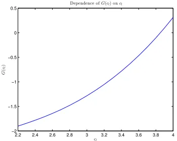
In constructing self-similar profiles in the previous section, we did not consider the decay condition (2.3.1b). In this subsection, we show that the decay condition determines the scaling exponentcl, i.e. only for certaincl do the constructed self-similar profiles satisfy the decay condition. Recall that for fixed leading order of Θ(ξ), s, and the value of the leading orderΘs = 1, the constructed profilesU(ξ), Θ(ξ) andW(ξ) depend oncl only. So we can define a functionG(cl) as

G(cl)= lim

ξ→+∞ U(ξ)

ξ .

We will prove that G(cl) < +∞ and it is a continuous function of cl. Then the existence ofcl to make the decay condition (2.3.1b) hold will follow from the In-termediate Value Theorem if we can show that there existcl_l andc_lr such that

G(cl_l) < 0, G(c_lr) > 0. (2.3.23)

Lemma 2.3.3. For fixed cl > 2and leading order ofΘ(ξ), s ≥ 2, construct power

series(2.3.4)withΘs =1, and extend the profiles toR+ using(2.3.17). Then G(cl) = lim

ξ→∞ U(ξ)

ξ <+∞, and G(cl)is a continuous function of cl.

For the convenience of analysis, we first make the following change of variables, η =ξ1/cl, _Wˆ (η) =_W(ξ), _Uˆ(η) =_U(ξ)ξ−1, Θ(ηˆ ₎= Θ(ξ)ξ−1+2/cl. _(2.3.24)

Then we have

G(cl) = lim

η→+∞ ˆ U(η), and the ODE system satisfied by ˆU(η),Θ(ηˆ ),Wˆ(η) is

ˆ

Θ0(η)= (2/cl−1) ˆΘ(η) ˆU(η)

η+1/cl_Uˆ_(η)η , (2.3.25a)

ˆ

W0(η)= −Wˆ (η) η+1/cl_Uˆ_(η_)η +

(1−2/cl) ˆΘ(η)

(1+1/clUˆ(η))2η3, (2.3.25b)

ˆ

U0(η)= clWˆ(η)

η . (2.3.25c)

According to (2.3.8), (2.3.16) and the fact that ˆU(η) is increasing, we have ˆ

U(η) >Uˆ(0)= (1−s)cl−2

s ,

ˆ

(32)

Lemma 2.3.4. For all cl > 2, G(cl) > −2.

Proof. Assume that for somecl > 2,G(cl) ≤ −2. Then, according to (2.3.26) and the fact that ˆU(η) is increasing, we have that for allη >0,

(1−s)cl−2 s <

ˆ

U(η) < −2.

Then we get

(2/cl −1) ˆU(η) 1+1/clUˆ(η) ≥ 2. It follows from (2.3.25a) that

ˆ

Θ0(η) ≥ 2Θ(η)ˆ η .

By direct integration and (2.3.26), we have that forηlarge enough, ˆ

Θ(η) ≥ C1η2.

Using this estimate and (2.3.26) in (2.3.25b), we get ˆ

W0(η) ≥ −C2Wˆ (η)

η +

C3

η .

This implies

ηC₂ _ˆ

W(η)0 _≥

C3ηC2−1.

Then we have that forη large enough, ηC2_Wˆ(η) _≥ C3

C2

ηC2 ₋_C

4.

Using this lower bound in (2.3.25c), we get ˆ

U0(η) ≥ C5

η − C6

ηC2+1. (2.3.27)

The constants C in the above estimates are positive and independent of η. The inequality (2.3.27) implies that ˆU(η) → +∞ asη → +∞, which contradicts with G(cl) ≤ −2. This completes the proof of Lemma 2.3.4.

We add a subscript cl to indicate the dependence of the constructed self-similar profiles on the parametercl for the rest part of this subsection:

ˆ

(33)

Lemma 2.3.5. For s ≥ 2 and cl > 2, choose Θs = 1 in constructing the power series(2.3.4), and extend the local profiles toR+ using(2.3.17). Then for fixed η,

ˆ

Uc_l(η),Wcˆ _l(η)andΘˆcl(η)are continuous as functions of cl.

Proof. We only need to prove for fixedc_l0 > 2, ˆUc_l(η), ˆΘc_l(η) and ˆWc_l(η) as func-tions ofcl are continuous atcl = c_l0. In our construction of the power series using (2.3.12), we can easily see that the coefficientsUk andΘk depend continuously on cl. And based on (2.3.13), there exist uniform upper bounds of the coefficients

|Uk| ≤ u

0_rk

k2 , |Θk| ≤

θ0_rk k ,

forclin a neighborhood ofc_l0. This means there exists a fixed small enough, such that ˆWc_l(), ˆΘc_l() and ˆUc_l() as functions ofcl are continuous atc_l0.

Then we can use the continuous dependence of ODE solutions on initial data and parameters to complete the proof of this lemma.

Now we begin to prove Lemma 2.3.3. We use an iterative method which enables us to get sharper estimates of the profiles after each iteration. We finally obtain that

ˆ

Uc_l(η) converges uniformly toG(cl) and complete the proof.

Proof. Considerc_l0> 2, and it is sufficient to prove thatG(c_l0) <+∞, andG(cl) as a function is continuous at the pointcl =c_l0.

According to Lemma 2.3.4 and Lemma 2.3.5, there existsη0large and a

neighbor-hood ofc0_l,I0= (c1,c2) withc1 > 2,c2 < +∞, such that forcl ∈ I0andη > η0,

ˆ

Uc_l(η) >Ucˆ _l(η0) >−2+1. (2.3.28)

Then forcl ∈ I0andη > η0, there exists2> 0, such that

(2/cl−1) ˆUc_l(η)

1+1/clUcˆ _l(η) < 2−2. Using this in (2.3.25a), we have that forcl ∈ I0andη > η0,

ˆ Θ0_c

l(η) ≤

(2−₂) ˆΘcl(η)

η .

Using direct integration and Lemma 2.3.5, we have that forcl ∈ I0,η > η0,

ˆ

Θcl(η) ≤C1η

(34)

Using this upper bound of ˆΘ(η) in (2.3.25b), we have that forcl ∈ I0,η > η0,

The first term in (2.3.29) is negative according to (2.3.26) and the second term is integrable forη > η0. Then using Lemma 2.3.5, we have that forcl ∈ I0,η > η0,

ˆ

Wc_l(η) <C4.

Putting this upper bound in (2.3.25c) and using Lemma 2.3.5, we get that ˆ

Uc_l(η) < C5lnη, cl ∈I0, η > η0.

Putting this upper bound of ˆU(η) back in (2.3.25b), we have that ˆ

Again putting this sharper upper bound in (2.3.25b), we have that ˆ

By direct integration, we get ˆ

Note thatC1,C2, . . .C15in the above estimates are all positive constants independent

of η. Using the upper bound of ˆWc_l(η) (2.3.30) in (2.3.25c), we conclude that ˆ

Uc_l(η) converges uniformly asη →+∞forcl ∈I0and complete the proof.

(35)

Existence of Self-Similar Profiles

In this subsection, we verify condition (2.3.23) for s = 2, i.e., there exist cl_l,cr_l > 2, such that G(cl_l) < 0, G(cr_l) > 0, with which we can complete the proof of the existence of self-similar profiles. The following lemma allows us to verify the conditions (2.3.23) using estimates of the profiles at some finiteη0.

Lemma 2.3.6. Consider solving equations(2.3.25)with initial conditions given by

power series(2.3.4). For someη0 > 0, let u0=Uˆ(η0), θ0= Θ(ηˆ 0),w0 =Wˆ(η0).

We prove the second part (2.3.31d) by contradiction. IfG(cl) ≥0, then there exists η1 ∈(η0,+∞] such that ˆU(η1) =0, and forη ∈ (η0,η1), ˆU(η) > u0.

(36)

Putting this upper bound of ˆW(η) in (2.3.25c) and integrating fromη0toη1, we get

0−u0=Uˆ(η1)−Uˆ(η0) ≤ clw0+

(cl−2)θ₀

(u0+2)(1+u0/cl)η2₀

,

which contradicts (2.3.31c). Then we complete the proof of this lemma.

Next we use numerical computation together with rigorous error control to verify the condition (2.3.31a) or (2.3.31c) for differentcl

Computer programs have been used to prove several important mathematical theo-rems including, to name a few, the four color theorem [1], Kepler conjecture [34] and some others [53, 45, 25]. One method of computer-assisted proof is to use the interval arithmetic and inclusion principle to ensure that the output of a numer-ical program encloses the solution of the original problem. One first reduces the computation to a sequence of the four elementary operations, and then proceeds by replacing numbers with intervals and performing elementary operations between such intervals of representable numbers under appropriate rounding rules.

To be precise, assume thatx ∈[xmin,xmax], y ∈ [ymin,ymax], where xmin, xmin, ymin

andymaxare floating point numbers that can be represented exactly on a computer.

Then for one of the four elementary operations, ∈ {+,−,∗,/}, we have

x y ∈[zmin,zmax], (2.3.34a)

where

zmin =min{xminymin,xminymax,xmaxymin,xmaxymax}, (2.3.34b)

zmax =max{xminymin,xminymax,xmaxymin,xmaxymax}, (2.3.34c)

and and refer to standard floating point operations with rounding modes set to ‘DOWNWARD’ and ‘UPWARD’ respectively [77]. Namely, xyis the largest floating number less thanxy, andxyis the smallest floating number larger than x y. For the case thatis division we require that 0_<[ymin,ymax].

The RHS of (2.3.34) involve only floating point operation, so (2.3.34) allows us to track the propagation of numerical errors using computer programs.

Using the above interval arithmetic strategy, we first numerically construct the power series (2.3.4) locally with Θs = 1, and then extend them to some η0 by

(37)

c_ll =3,c_lr =8. But the same process can be applied to others > 2 to verify the exis-tence of self-similar profiles. The computer programs used for this part of proof can be found athttps://sites.google.com/site/pengfeiliuc/home/codes. We first consider the cases= 2,cl =3, and verify that fors= 2,G(3) <0.

Step 1 We need to control the numerical error in the local power series solutions. To numerically compute (2.3.4), we first truncate the power series to finite terms. For the cases =2,cl =3, the following choice ofθ0,u0andrmakes (2.3.13) hold: Using estimates (2.3.14), if we truncate the power series (2.3.35) tom = 20 terms, the truncation errors of the three series can be bounded respectively by

u0rm+1η3sm Then we need to estimate the truncated power series

ˆ

Using the interval arithmetic (2.3.34) strategy in each elementary operation of (2.3.12), we can inductively get computer representable intervals enclosing the values ofUk and Θk for all k ≤ 21. Then we use these intervals in computing (2.3.37) to get intervals enclosing the values of the truncated power series (2.3.37). Finally we add back the the intervals (2.3.36) enclosing the truncation errors using interval arithmetic, and get intervals strictly enclosing ˆU(ηs), ˆW(ηs) and ˆΘ(ηs).

and use them as initial conditions to solve (2.3.25).

We use the forward Euler scheme [56] to numerically integrate the ODE system (2.3.25). For a general ODE system with given initial data,

y = (y1(x),y2(x), . . .yN(x))T, y0(x)= f(x,y), x ∈[a,b], y(a)= y0,

(38)

the forward Euler scheme discretizes the domain to finite points, a = x0 < x1· · ·< xm =b

with step size xi− xi−1 = h, and the numerical solutions yn ≈ y(xn) are obtained by

yn+1 = yn+h f(xn,yn). (2.3.40) For the solution of the ODE system (2.3.39), using Taylor expansion, we have

y(xn₊1) = y(xn)+h f(xn,y(xn))+1/2

previous steps andI2is the local truncation error of the integration scheme.

We solve (2.3.25) from ηs = 10−1 toη0 = 3 with step size h = 2.9× 10−6, and

denote the node point and solutions at then-th step as ηn₌ _0.1₊_nh,

Step 2We need to control the roundofferror in computingyn+1(2.3.40). In then-th

step, we have intervals In_ˆ U, I

Θ that enclose the values of the profiles atη

n_. To update these intervals, we first choose the middle points of these intervals, and use them as the numerical solution yn. Then we use interval arithmetic to update (2.3.40) to get intervals enclosing the numerical solutions yn+1at then+1-th step.

Step 3We need to control the propagation of error from previous steps,I1. Note that

(39)

their middle points as the numerical solution yn. So we use interval arithmetic to deduct the middle points from these intervals and get intervals enclosing y(xn)−yn in (2.3.42). Then we need estimates of the Jacobian matrix of (2.3.25), which is

∂ Using intervalsIn_ˆ

U,I

Θ and interval arithmetic in computing (2.3.44), we can get

intervals enclosing each entry of∇_yf(x,y∗) in (2.3.42). Then using interval arith-metic in computing∇_yf(x,y∗) y(xn)−yn gives us intervals enclosingI1.

Step 4 We need to control the local truncation errorsI2of the scheme, which are

1

To controlI2(2.3.45), we need the followinga prioriestimates.

Lemma 2.3.7. Consider the ODE system(2.3.25)with cl > 2and initial data given

(40)

Proof. According to (2.3.25a) and the lower bound of ˆU(η) (2.3.26), we have By direct integration, we can getθmaxandθmin.

ˆ

U(η) is increasing according to (2.3.25c), so we get the lower bound umin. Then

using the upper boundθmaxand (2.3.26) in (2.3.25b), we get

ˆ

W0(η) ≤ s

2_cl_θ max

(cl−2)(ηn₎3. (2.3.48)

By direct integration we get the upper bound wmax. Putting the upper bound of

ˆ

W(η) in (2.3.25c), we get the upper bound of ˆU(η),umax. Using the upper bound

wmaxand the lower boundumin in (2.3.25b), we have

ˆ

Remark 2.3.2. The a prioriestimates (2.3.47) that we get are relatively sharp for smallhsince they deviate from the values of the profiles only byO(h).

We first use intervals In_ˆ U, I

Θ and the interval arithmetic in (2.3.47) to get

intervals enclosing the values of the profiles in [ηn_,ηn+1_{]. Then we can use these}

intervals and interval arithmetic in (2.3.46a) to get an interval enclosing the local truncation error (2.3.45),I2.

Step 5 Finally, adding up the intervals enclosing the numerical solutions yn+1

(Step 2), the intervals enclosing the propagation of errors from previous steps I1

(Step 3), and the intervals enclosing the local truncation error I2 (Step 4), we get

intervals enclosing the values of the profiles atηn+1,In_ˆ+1

these intervals, we finally get estimates of the self-similar profiles atη =3: ˆ

U(3) ∈[−1.61167791024607,−1.61167791022341],

ˆ

W(3) ∈[0.110808868817194,1.10808868851010],

ˆ

Θ(3) ∈[0.934100399788941,9.34100399819680],

(41)

Remark 2.3.3. Since ˆWn, ˆUn and ˆΘn are enclosed in the intervals In_ˆ W, I

n

ˆ

U and I n

ˆ

Θ,

we can directly use interval arithmetic in (2.3.40) to get intervals enclosingy(xn)+ h f(xn,y(xn)). This strategy avoids estimating the Jacobian matrix∇_yf(x,y), but will amplify the propagation of errors from previous steps.

Next we consider the cases =2,cl=8, and verify that fors =2,G(8) >0.

The verification ofG(8) > 0 can be done in the same way. In the construction of the local solutions (2.3.4), we can easily verify that the choice of

u0= 1 6, Θ

0 ₌ 1

18, r =6

makes the constraint (2.3.13) hold. Then we truncate the power series (2.3.4) to the first 20 terms and evaluate them atηs = 0.7. Using the same technique as the case cl =3, we can get intervals enclosing the self-similar profiles atηs = 0.7

I0_ˆ W, I

0 ˆ

U, I

0 ˆ

Θ. (2.3.49)

Then we begin to numerically solve (2.3.25) using (2.3.49). We use the same tech-niques as the previous case to control the numerical errors introduced in each step of the integration, and finally get intervals enclosing the profiles atη= 3:

ˆ

U(3) ∈[5.66176313743309,5.66176313745025],

ˆ

W(3) ∈[1.13763978495371,1.13763978496956],

ˆ

Θ(3) ∈[2.54776073991655,2.54776074039048],

from which (2.3.31a) follows and we complete the proof that fors= 2,G(8)> 0. WithG(3) < 0,G(8)> 0, we conclude that there existsclsuch that the self-similar equations (3.1.5) have solutions with the leading order ofΘ(ξ) atξ =0 beings= 2. Remark2.3.4. We only verify the existence of self-similar profiles fors = 2. But the same procedure can be applied to the casess >2 without difficulty.

Behavior of the Self-Similar Profiles at Infinity

In this subsection, we prove that the constructed self-similar profiles satisfy the matching condition (2.2.6), and that the profiles are analytic with respect to a trans-formed variable ζ = ξ−1/cl _at ζ = _{0. With this we can complete the proof of}

(42)

Lemma 2.3.8. For some cl > 2 and s ≥ 2, if the self-similar profiles constructed using power series(2.3.4)and extended to the whole R+satisfy the decay condition (2.3.1b), then the profiles satisfy the matching condition(2.2.6).

After the following change of variables,

ζ = ξ−1/cl, _U˜(ζ₎=_U(ξ)ξ−1+1/cl, Θ(ζ˜ ₎ =Θ(ξ)ξ−1+2/cl, _W˜ (ζ) =_W(ξ)ξ1/cl,

(2.3.50) ˜

U(ζ),W˜(ζ) andΘ(ζ˜ )are analytic functions atζ =0.

Our strategy is the following: we first prove that ˜U(ζ), ˜W(ζ) and ˜Θ(ζ) are smooth at [0,+∞). Then we show that there exist analytic solutions to the ODE system of

˜

U(ζ), ˜W(ζ), ˜Θ(ζ) with the same initial conditions atζ = 0. Finally we show that smooth solutions to the ODE system of ˜U(ζ), ˜W(ζ), ˜Θ(ζ) with the given initial conditions are unique, with which we can complete the proof.

Proof. If the decay condition (2.3.1b) holds, then ˆU(η) tends to 0 in equation (2.3.25), and there existsη0 > 0 such that forη > η0, we have

(2/cl −1) ˆU(η)

1+1/clUˆ(η) ∈ (0,1/2). Then based on (2.3.25a), we have that forη > η0,

ˆ

Θ0(η) ≤ 1/2 ˆΘ(η)

η ,

which implies that forη > η0,

ˆ

Θ(η) ≤ C1η1/2. (2.3.51)

Using this estimate in (2.3.25b), we have that forη > η0,

ˆ

W(η)η0_≤

C2η−3/2,

which gives

ˆ

W(η)η <C3. (2.3.52)

Using the above estimate in (2.3.25c), we get that forη > η0,

ˆ

U0(η) ≤C4η−2,

which together with ˆU(+∞)= 0 implies that forη > η0,

ˆ

(43)

Based on (2.3.25b) and (2.3.25c), we have

with initial data given by (2.3.55) and (2.3.56), ˜

W(0)=W∞,ˆ Θ(0)˜ =Θ∞,ˆ U˜(0)=−clW∞.ˆ (2.3.57d)

Equation (2.3.57c) can be written as ˜ Using a simple bootstrap argument, we can get that

˜

W(ζ),Θ(ζ˜ ),U˜(ζ) ∈C∞ [0,+∞).

On the other hand, given the initial data (2.3.57d), we can construct the following power series solutions to equations (2.3.57):

(44)

Plugging these power series ansatz in (2.3.57) and matching the coefficients ofζk, we can uniquely determine the coefficients ˜Uk, ˜Wk, ˜Θk and prove that the power series (2.3.58) converge in a small neighborhood ofζ =0. We omit the details here, because the argument is the same as in the near-field. Then to prove the analyticity of ˜U(ζ), ˜W(ζ) and ˜Θ(ζ) atζ =0, we only need the uniqueness of smooth solutions to (2.3.57) with initial condition (2.3.57d). The RHS of (2.3.57c) is not Lipschitz, so the classical uniqueness result will not apply directly here.

Assume ˜Ui(ζ), ˜Wi(ζ), ˜Θi(ζ),i = 1,2, are two solutions to equation (2.3.57) with initial condition (2.3.57d). LetδU(ζ),δW(ζ),δΘ(ζ) be their differences,

δ_U˜_(ζ₎ ₌_U˜1_(ζ

)−U˜2(ζ), δW˜(ζ)=W˜1(ζ)−W˜2(ζ), δΘ(ζ)˜ =Θ˜1(ζ)−Θ˜2(ζ). Then based on (2.3.57c),

δU(ζ) =−cl

ζ

Z ζ

0

δW(ζ)dζ.

Using Hardy inequality[30], there existsC1independent of such that

kδU˜k_L2_([0_,_]) ≤ C₁kδW˜k_L2_([0_,_]).

Since the RHS of (2.3.57a) and (2.3.57b) are Lipschitz continuous, we have

| d

dζ(δW˜(ζ))|+| d

dζ(δΘ(ζ)))˜ | ≤C2(|δW˜(ζ)|+|δU˜(ζ)|+|δΘ(ζ˜ )|).

Integrating the square of both sides on the interval [0, ] and using (2.3), we get

k δW˜(ζ)0_k

L2_([0_,_])+k δΘ(ζ˜ )0k_L2_([0_,_]) ≤ C₃(kδW˜(ζ)k_L2_([0_,_])+kδΘ(ζ˜ )k_L2_([0_,_])).

(2.3.59) SinceδW˜(ζ) andδΘ(ζ˜ ) vanish atζ = 0, by Poincaré-Friedrichs inequality we have

kδW˜ (ζ)k_L2_([0_,_])+kδΘ(ζ˜ )k_L2_([0_,_]) ≤ C₄(k δW˜(ζ)0k_L2_([0_,_])+k δΘ(ζ˜ )0k_L2_([0_,_])).

(2.3.60) TheC in the above estimates are all positive constants independent of. Choosing small enough, we get a contradiction between (2.3.59) and (2.3.60), and thus

˜

W1 =W˜2, U˜1=U˜2, Θ˜1= Θ˜2,

(45)

Numerical Results

In this subsection we numerically locate the root ofG(cl) for severalsand construct the corresponding self-similar profiles. Then we compare the obtained cl and self-similar profiles with direct numerical simulation of the CKY model.

For any fixedcl > 2, we first numerically compute the coefficientsΘk,Ukin (2.3.4) up to k = 50 and determine the convergence radius of the power series using the following linear regression fors ≤ k ≤ 50,

logΘk = klogr1+c1, logUk = klogr2+c2. (2.3.61)

We chooser = 1/2 min{1/r₁,1/r₂}and construct (2.3.4) on [0,r/2].

Then we solve equation (2.2.4) from ξ = r/2 to ξ = 1 using the 4th order Runge-Kutta method with step-size h= 1−r₁₀4/2.

After ξ = 1, we make the change of variables (2.3.24) and solve the ODE system (2.3.25) fromη = 1 toη =105using 4th order Runge-Kutta method with step-size h= 105−1

106 . We use ˆUcl(10

5_{) as an approximation to}_G(cl).

We use the bisection method to find the root ofG(cl).

After getting cl, we construct the local self-similar profiles using power series (2.3.4) and extend them fromξ =r/2 toξ =10 using the explicit 4th order Runge-Kutta method with step-sizeh= 9

104. Then we locate the maximum ofW, which is

We only compare the self-similar profiles Ws with direct simulation of the CKY model in this thesis, but the numerical results for the profilesΘandU are similar. We use a particle method in the direct simulation of the CKY model and consider N +1 particles with position, density and vorticity given by



(46)

In computing the driving force ofw, which isθx, we use the three points rule:

Initially, 105+1 particles are equally placed in the short interval [0,10−3], which are sufficient to resolve the solutions in the self-similar regime. Outside this short interval 105−102particles are equally placed. So the total number of particles is

N +1= 2×105−102.

Then we need to solve the following ODE system d

The initial condition ofθis

θ(x,0) = (1−cos(πx))s/2, whose leading order atx = 0 iss.

We solve the ODE system (2.3.63) using the 4-th order Runge-Kutta method, and the time stepdtis chosen adaptively to avoid particle-crossing:

dti = 1

At each time step, we record the maximal vorticitywmax(ti), and the position where

it is attainedqmax(ti). According to the self-similar ansatz (2.2.2), we have

wmax(t)=C1(T−t)cw, qmax(t) =C2(T −t)cl.

Thus we can computecl,cw, and the singularity timeT through linear regressions, d

We compute the time derivatives of logwmax(t) and logqmax(t) using the center

(47)

s= 2 s= 3 s=4 s =5 cw −0.9747 −1.0001 −1.0006 −1.0007

Table 2.1: Scaling exponentcwobtained from direct numerical simulation.

At certain time steps close to the singularity time,ti,i = 1,2,3, letwi be the maxi-mal vorticity at timetiandqi be the position the maximal vorticity is attained. We rescale the numerical solution and get the self-similar profiles ofw,

Wsi(ξ) = 1

wmax

w(ξqi,ti), ξ ∈[0,1]. (2.3.65)

We compare the profiles W_si(ξ) (2.3.65) obtained from direct simulation of the model, withWs(ξ) (2.3.62) obtained from the self-similar equations (3.1.5). Near singularity time the velocity field seems to be Hölder continuous at the origin,

u(x,T) ≈C xα.

Then we can determine the Hölder exponentαthrough linear regression

lnu(x,T)≈ lnC+αlnx. (2.3.66)

We will compare the exponents α (2.3.66) obtained from the singular solutions, with 1−1/cl obtained from analyzing the self-similar equations (3.1.5).

In simulating the CKY model, we choosew(x,0) as

w(x,0) =1−cos(4πx). (2.3.67) We compute the scaling exponents cw andcl for different leading orders ofθ, s = 2,3,4,5, using (2.3.64a) and (2.3.64b), and the results are listed in Table 2.1 and Table 2.2. The Hölder exponents of the velocity field at the singularity time (2.3.66) and 1−1/cl are listed in Table 2.3. The cl that we use in computing 1−1/cl are obtained from solving the self-similar equations.

From the Table 2.1, 2.2, 2.3, we can see that the exponentscw we obtain from the numerical solutions are close to−1. And theclwe obtain from the singular solution (2.3.64b) are close to those obtained from solving the self-similar equations. At the singularity time, the Hölder exponents of the velocity field are close to 1−1/cl.

(48)

.

2.2 2.4 2.6 2.8 3 3.2 3.4 3.6 3.8 4

−2 −1.5 −1 −0.5 0 0.5

cl

G

(

cl

)

Dependence ofG(cl) oncl

Figure 2.2: Dependence ofG(cl) oncl fors= 2. s= 2 s =3 s= 4 s =5 Linear Regression 3.7942 3.3143 3.1718 3.0773 Self-Similar Equations 3.7967 3.3157 3.1597 3.0841

Table 2.2: cl got from linear regression (2.3.64b) and the self-similar equations.

s= 2 s =3 s=4 s= 5

Hölder exponent 7.3381×10−1 6.9823×10−1 6.9131×10−1 6.7610×10−1 1−1/cl 7.3661×10−1 6.9841×10−1 6.8351×10−1 6.7576×10−1

Table 2.3: Hölder exponent of the velocity field at the origin.

fixeds, the scaling exponentclto make the decay condition (2.3.1b) hold is unique.

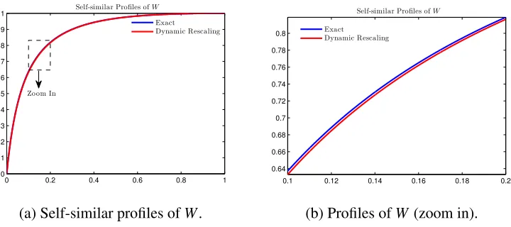
The self-similar profiles that are obtained from solving the self-similar equation (2.3.62) and from direct simulation of the model (2.3.65) are plotted in Figure 2.3. The lines labeled ‘exact’ are obtained from solving the self-similar equation (2.3.62). Others profiles are obtained from rescaling the numerical solutions at different time steps corresponding to different maximal vorticity (2.3.65).

(49)

0 0.1 0.2 0.3 0.4 0.5 0.6 0.7 0.8 0.9 1

(a) The re-scaled solutions and self-similar

profiles we construct. s=2.

0 0.1 0.2 0.3 0.4 0.5 0.6 0.7 0.8 0.9 1

(b) The re-scaled solutions and self-similar

0 0.1 0.2 0.3 0.4 0.5 0.6 0.7 0.8 0.9 1

(c) The re-scaled solutions and self-similar

0 0.1 0.2 0.3 0.4 0.5 0.6 0.7 0.8 0.9 1

(d) The re-scaled solutions and self-similar

Figure 2.3: Self-similar profiles ofW fors= 2,3,4,5.

2.4 Stability of the Self-similar Profiles