Subclasses of Tree Adjoining Grammar for RNA Secondary Structure

Subclasses of Tree Adjoining Grammar for RNA Secondary Structure

Yuki Kato

Graduate School of

Information Science,

Nara Institute of

Science and Technology

Takayama 8916-5, Ikoma,

Nara 630-0192, Japan

[email protected]

Hiroyuki Seki

Graduate School of

Information Science,

Nara Institute of

Science and Technology

Takayama 8916-5, Ikoma,

Nara 630-0192, Japan

[email protected]

Tadao Kasami

Graduate School of

Information Science,

Nara Institute of

Science and Technology

Takayama 8916-5, Ikoma,

Nara 630-0192, Japan

[email protected]

Abstract

Several grammars have been proposed for rep-resenting RNA secondary structure including pseudoknots. In this paper, we introduce subclasses of multiple context-free grammars which are weakly equivalent to these grammars for RNA, and clarify the generative power of these grammars as well as closure property.

1

Introduction

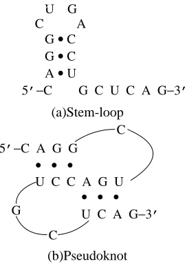
Much attention has been paid to RNA secondary struc-ture prediction techniques based on context-free grammar (cfg) since cfg can represent stem-loop structure (Fig-ure 1 (a)) by its derivation tree and recognition (or

sec-ondary structure prediction in biological words) can be

performed inO(n3_{)time wherenis the length of an}

in-put sequence (primary structure). Especially, techniques based on CKY (Cocke-Kasami-Younger) algorithm have been widely investigated (Durbin et al., 1998).

Pseu-doknot (Figure 1 (b)) is one of the typical substructures

found in an RNA secondary structure. An alternative rep-resentation of a pseudoknot is arc depiction in which arcs cross (see Figure 2). It has been recognized that pseu-doknots play an important role in RNA functions such as ribosomal frameshifting and splicing. However, it is known that cfg cannot represent pseudoknot structure.

In bioinformatics, a few grammars have been proposed to represent pseudoknots (Uemura et al., 1999; Rivas and Eddy, 2000) (also see (Condon, 2003)). In the pioneer-ing paper, Uemura et al. (1999) define two subclasses of tree adjoining grammar (tag) called sl-tag and esl-tag, and argue that esl-tag is appropriate for representing RNA secondary structure including pseudoknots. Rivas and Eddy (2000) provide keen observation on representation of RNA secondary structure by a sequence with a single “hole” and introduce a new class of grammars for deriv-ing sequences with hole. These grammars have

gener-ative power stronger than cfg while recognition can be performed in polynomial time. However, relation among the generative power of these grammars and/or mildly csg has not been clarified.

In this paper, we identify grammars for RNA sec-ondary structure (Uemura et al., 1999; Rivas and Eddy, 2000) as subclasses of multiple context-free grammar (mcfg) (Kasami et al., 1988a; Seki et al., 1991) and clar-ify inclusion relation among the classes of languages gen-erated by these grammars.

The rest of this paper is organized as follows. Section 2 reviews the grammars mentioned above. In section 3, these grammars are characterized as subclasses of mcfg. Generative power and closure property of these grammars are discussed in section 4. Section 5 concludes the paper.

U G C A G • C G • C A • U

5’−C G C U C A G−3’ (a)Stem-loop

5’−C A G G • • •

U C C A G U • • •

U C A G−3’

C

G C

(b)Pseudoknot

c a g g c u g a c c u g c u c a g

Figure 2: Arc depiction of Figure 1 (b)

2

Preliminaries

2.1 Tree Adjoining Grammar

We will use standard notations for tree adjoining gram-mar (Joshi and Schabes, 1997). The empty sequence is denoted byε. For a sequenceα∈S∗_{, let|α|denote the} length ofα.

A tree adjoining grammar (tag) is a 5-tuple G = (N, T, S,I,A)whereN andT are finite sets of nonter-minals and ternonter-minals respectively,S the start symbol,I a finite set of initial trees (center trees) andA a finite set of adjunct trees (auxiliary trees). The path of an ad-junct tree from the root node to the foot node is called the backbone. Selective adjoining (SA), null adjoining (NA) and obligatory adjoining (OA) are defined in the standard way. For treessandt, ift0 is obtained by ad-joiningsintot, we writet `s t0 (or simplyt ` t0). We write the reflective and transitive closure of`as`∗_{. We} callt0 <sub>a derived tree (or a tree derived fromt) ift `</sub>∗ <sub>t</sub>0 for somet∈ I ∪ A. A nodenis inactive if the constraint for the node is NA, otherwise active. If no active node in a treethas OA constraint, thentis called mature. The tree set of a tagGis defined asT(G) ={t|s`∗ _{t, s∈} Iandtis mature}. T(G)can be alternatively character-ized in a bottom up way as follows. Let us define a series of tree setsT0(G), T1(G), . . ..

(T1) T0(G) ={t∈ I ∪ A |tis mature}.

(T2) Tn+1(G) = Tn(G)∪ {t | t0 `s1 t1 `s2 · · · `sk

tk = t, t0 ∈ I ∪ A, si ∈ Tn(G) (1 ≤ i ≤

k), p1, . . . , pkare different addresses oft0, siis

adjoinable tot0atpi(1≤i≤k)andtis mature}.

It is not difficult to show that T(G) = {t | t ∈ Tn(G)for somen≥0and yield(t)∈T∗}. This charac-terization ofT(G)by (T1) and (T2) is frequently used in proofs in section 3.

The language generated byG is defined as L(G) = {w | w = yield(t), t ∈ T(G)}, which is called a tree

adjoining language (tal). Let TAG denote the class of

tags and TAL denote the class of tals. We use the same notational convention, i.e., a language generated by an xxg is called an xxl, the class of xxgs is denoted by XXG and the class of xxls is denoted by XXL.

We now define simple linear tag (sl-tag) and extended

simple linear tag (esl-tag) introduced in (Uemura et al.,

1999). LetG= (N, T, S,I,A)be a tag. An elementary tree is simple linear if it has exactly one active node, and

for an adjunct tree, the active node is on the backbone of the tree. A tagGis a simple linear tag (sl-tag) if and only if all elementary trees inGare simple linear. An adjunct tree is semi-simple linear if it has two active nodes, where one is on the backbone and the other is elsewhere. A tag Gis an extended simple linear tag (esl-tag) if and only if all initial trees inGare simple linear and all adjunct trees inGare either simple linear or semi-simple linear. Example 1 (Uemura et al., 1999). Let G = (N, T, S,I,A) be an sl-tag where N = {S}, T = {a, c, g, u} and elementary trees inI andAare shown in Figure 3. In the figure, z ∈ {a, c, g, u}, (x, y) ∈ {(a, u),(u, a),(c, g),(g, c)} and an active node is de-noted byS∗. Figure 4 shows a derivation of a pseudo-knot.

S S*

x y

S S*

z S

S* z

S S* x

S y

S S* x

S y

Initial tree Adjunct trees

ε

S*

S

z S

*

S

x y

S z

S*

S*

Figure 3: Elementary trees in Example 1

ε

S* _S

S* a u

ε

S

S

S a

u

ε

S S g

c S

*

S

S a

u

ε

S S g

c S

*

a S u

a g a c u u

Figure 4: A derivation of a pseudoknot in Example 1

By definition,

SL-TAL⊆ESL-TAL⊆TAL. (∗1)

On the inclusion relation among CFL, SL-TAL and ESL-TAL, the following has been shown in Propositions 1 to 3 of (Uemura et al., 1999):

L2={]ak1bk1]al2bl2]am3bm3]an4bn4]|k, l, m, n≥1}

∈CFL\SL-TAL, (∗2)

{anbncn|n≥0} ∈SL-TAL\CFL, (∗3)

2.2 Multiple Context-Free Grammar

A multiple context-free grammar (mcfg) or linear

context-free rewriting system (Vijay-Shanker et al., 1987)

is a 5-tupleG= (N, T, F, P, S)whereN is a finite set of nonterminals,T a finite set of terminals,Fa finite set of functions,Pa finite set of (production) rules andSthe start symbol. For eachA∈N, a positive integer denoted asdim(A)is given andAderivesdim(A)-tuples of ter-minal sequences. For the start symbolS,dim(S) = 1. For eachf ∈ F, positive integers di (0 ≤ i ≤ k)are given andf is a total function from(T∗₎d1_{×· · ·×(T}∗₎dk to(T∗₎d0_{which satisfies the following condition (F):} (F) Letxi = (xi1, . . . , xidi)denote theith argument of

f for1 ≤ i ≤ k. Thehth component of function value for1≤h≤d0, denoted byf[h], is defined as

f[h][x1, . . . , xk] =βh0zh1βh1zh2· · ·zhvhβhvh (∗)

whereβhl∈T∗_{(0≤l ≤vh)andzhl∈ {xij |1≤} i≤k, 1≤j≤di}(1≤l≤vh). The total number of occurrences ofxij in the right hand sides of (∗) fromh= 1throughd0is at most one.

Each rule in P has the form of A0 → f[A1, . . . , Ak]

whereAi ∈N(0≤i≤k)andf : (T∗)dim(A1)× · · · ×

(T∗₎dim(Ak)→(T∗)dim(A0)∈F_{. If}k≥1_{, then the rule} is called a nonterminating rule, and ifk = 0, then it is called a terminating rule.

We define the relation⇒∗ and derivation trees (refer to Figure 5) recursively by the following (L1) and (L2):

(L1) IfA →α∈ P (α∈T∗_{), thenA⇒}∗ _{αand a tree} with the single node labeledA : αis a derivation tree forα.

(L2) If A → f[A1, . . . , Ak] ∈ P, Ai ⇒∗ αi =

(αi1, . . . , αidim(Ai)) (1 ≤ i ≤ k) andt1, . . . , tk are derivation trees for α1, . . . , αk, then A ⇒∗

f[α1, . . . , αk] where f[α1, . . . , αk] denotes the

dim(A)-tuple of terminal sequences obtained from the right hand sides of (∗) in condition (F) by sub-stitutingαij (1 ≤ i ≤k, 1 ≤ j ≤ dim(Ai))into xij, and a tree with the root labeledA:fwhich has t1, . . . , tkas (immediate) subtrees from left to right

is a derivation tree forf[α1, . . . , αk].

The language generated by an mcfg G is defined as L(G) ={w∈T∗_{|S ⇒}∗ _w}.

To introduce subclasses of MCFG, we define a few terminologies. LetG = (N, T, F, P, S)be an arbitrary mcfg. The dimension of G is defined as dim(G) =

max{dim(A) | A ∈ N}. For a function f ∈ F, let rank(f)denote the number of arguments off. The rank ofGis defined as rank(G) = max{rank(f) | f ∈ F}.

For a functionf : (T∗)d1 × · · · ×(T∗)dk → (T∗)d0_, let deg(f) = Σk_j=0dj, which is called the degree of f. Finally, let us define the degree ofGas deg(G) =

max{deg(f) | f ∈ F}. By definition, deg(G) ≤

dim(G)(rank(G) + 1). With these parameters, we de-fine subclasses of MCFG. An mcfgGwithdim(G)≤m and rank(G)≤ris called an(m, r)-mcfg. Likewise, an mcfgGwithdim(G)≤mis called anm-mcfg.

It has been proved that

TAL⊂(2,2)-MCFL⊂2-MCFL⊂MCFL, (∗5)

where the proper inclusion relation from left to right in (∗5) were given by Lemma 4.15 of (Seki et al., 1991), Theorem 1 of (Rambow and Satta, 1994) and Lemma 5 of (Kasami et al., 1988a), respectively.

Example 2. Consider the (2,2)-mcfg

G3 = ({S, A},{a, c, g, u}, F3, P3, S) for generating

RNA sequences, whereP3andF3are as follows:

S→J[A],

A→XS1[A, A]|XS2[A, A]|XS3[A, A],

A→BF1[A, A]|BF2[A, A]|BF3[A, A],

A→BPαβ[A]

((α, β)∈ {(a, u),(u, a),(c, g),(g, c)}),

A→U Pα1,L[A]|U Pα1,R[A]|U Pα2,L[A]|U Pα2,R[A]

(α∈ {a, c, g, u}), A→(ε, ε),

J[(x1, x2)] =x1x2,

XS1[(x11, x12),(x21, x22)] = (x11, x21x12x22),

XS2[(x11, x12),(x21, x22)] = (x11x21, x12x22),

XS3[(x11, x12),(x21, x22)] = (x11x21x12, x22),

BF1[(x11, x12),(x21, x22)] = (x11, x12x21x22),

BF2[(x11, x12),(x21, x22)] = (x11x12, x21x22),

BF3[(x11, x12),(x21, x22)] = (x11x12x21, x22),

BPαβ[(x1, x2)] = (αx1, x2β),

U Pα1,L[(x1, x2)] = (αx1, x2),

U P1,R

α [(x1, x2)] = (x1α, x2),

U P2,L

α [(x1, x2)] = (x1, αx2),

U Pα2,R[(x1, x2)] = (x1, x2α).

J[(aga, cuu)] = agacuu. G3 has a derivation tree

(Figure 5) foragacuuwhich represents the pseudoknot shown in Figure 4.

S : J

A : XS2

A : BPau A : BPau A : BPgc

A : (ε, ε)

A : (ε, ε)

Figure 5: A derivation tree inG3

Recognition problem for mcfg can be solved in poly-nomial time:

Proposition 1 (Kasami et al., 1988b; Seki et al., 1991). LetGbe an mcfg withdeg(G) =e. For a givenw∈T∗, whetherw∈L(G)or not can be decided inO(ne)time wheren=|w|.

3

Subclasses of MCFG

3.1 A Subclass of MCFG for SL-TAL

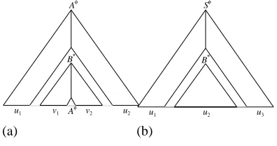
Grammars G and G0 are called weakly equivalent if L(G) = L(G0_{). Remember that each elementary tree} in an sl-tag contains exactly one active node as shown in Figure 6 (An inactive node and an active node are denoted likeAφandB∗, respectively in the figure). By utilizing this restriction, we can define a translation from an sl-tag into a weakly equivalent (2,2)-mcfg simpler than that of (Vijay-Shanker et al., 1986). Namely, for an adjunct tree in Figure 6 (a), construct an mcfg ruleA→f[B]where f[(x1, x2)] = (u1x1v1, v2x2u2). This translation

moti-vates us to define the following subclass of (2,1)-MCFG.

Aφ

Aφ

u1 v1 v2 u2

B*

(a)

Sφ

u1 u2 B*

u3

(b)

Figure 6: Elementary trees in sl-tag

Definition 1. A (2,1)-mcfgG = (N, T, F, P, S0)is an sl-mcfg ifGsatisfies the following conditions (1) and (2):

(1) For each nonterminalAother thanS0,dim(A) = 2.

(2) Each nonterminating rule has the form of either S0 → J[A] whereJ[(x1, x2)] = x1x2 or A →

f[B]where A, B ∈ N \ {S0} andf[(x1, x2)] =

(u1x1v1, v2x2u2)for someuj, vj ∈T∗(j= 1,2).

Such a function f is called a simple linear

func-tion.

Lemma 2. SL-TAL=SL-MCFL.

Proof. (SL-TAL⊆SL-MCFL)LetG= (N, T, S,I,A) be a given sl-tag. We will construct an sl-mcfgG0 =

(N0_{, T, F, P, S}

0)as follows:

(1) N0 _{=N∪ {S}

0}wheredim(S0) = 1anddim(A) =

2for eachA∈N.

(2) P (and F) are the smallest sets which satisfy the following conditions (a) through (c):

(a) S0→J[S]∈PandJ ∈F.

(b) For each adjunct treet∈ Ashown in Figure 6 (a),

• A → f[B] ∈ P and f ∈ F where f[(x1, x2)] = (u1x1v1, v2x2u2), and

• A→(u1v1, v2u2)ifBin Figure 6 (a) does

not have OA constraint (i.e.,tis mature). (c) For each initial treet ∈ I shown in Figure 6

(b),

• S → g[B] ∈ P and g ∈ F where g[(x1, x2)] = (u1x1u2, x2u3), and

• S→(u1u2, u3)iftis mature.

We can show that there exists a treet∈Tn(G)for some n≥0such that yield(t) =w1Aw2 (A ∈N, w1, w2 ∈

T∗_{)if and only ifA⇒}∗

G0 (w₁, w₂).

(SL-MCFL ⊆ SL-TAL) Let G = (N, T, F, P, S0)

be a given sl-mcfg. Construct an sl-tag G0 ₌

(N0_{, T, S}

0,I,A)as follows:

(1) N0 =N∪ {X}whereX 6∈N.

(2) I consists of initial trees shown in Figure 7 (a) for S0→J[A]∈P.

(3) Ais the smallest set satisfying:

• For eachA→f[B]∈P wheref[(x1, x2)] =

(u1x1v1, v2x2u2), the adjunct tree shown in

Figure 6 (a) belongs toA.

• For eachA → (u1, u2) ∈ P, the adjunct tree

in Figure 7 (b) belongs toA.

S0

AOA

ε (a)

Aφ

u1 Aφ u2

X*

(b)

Figure 7: Constructed elementary trees

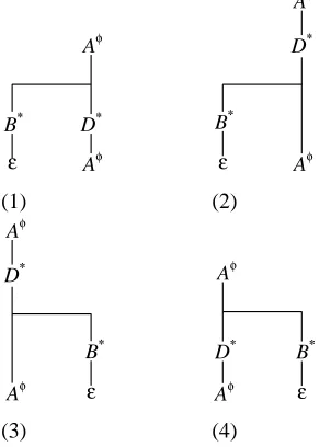
3.2 A Subclass of MCFG for ESL-TAL

In this subsection, we will define a subclass of (2,2)-MCFG which exactly generates ESL-TAL. Let G = (N, T, S,I,A)be a given esl-tag. By virtue of Property 2 of (Uemura et al., 1999), we can assume thatGis in normal form such that for every semi-simple linear ad-junct treet ∈ A, yield(t) ∈ N. Thus, for each leafv oft, eithervis the foot node or the label of visε(see Figure 8). From this observation, we define a subclass of (2,2)-MCFG by adding rules corresponding to adjunct trees shown in Figure 8 to the definition of sl-mcfg.

Aφ

Aφ D* B*

ε

(1)

Aφ

Aφ D*

B*

ε (2)

Aφ

Aφ D*

B*

ε

(3)

Aφ

Aφ

D* _B*

ε (4)

Figure 8: Semi-simple linear adjunct trees in normal form

Definition 2. A (2,2)-mcfgG = (N, T, F, P, S0)is an esl-mcfg if each nonterminating rule has one of the

fol-lowing forms (1) through (3):

(1) A→J[B]wheredim(A) = 1anddim(B) = 2.

(2) A→f[B]wherefis a simple linear function.

(3) A → g[B, D] where dim(A) = dim(D) = 2,

dim(B) = 1,g∈ {C1, C2, C3, C4}and

C1[x1,(x21, x22)] = (x1x21, x22),

C2[x1,(x21, x22)] = (x21x1, x22),

C3[x1,(x21, x22)] = (x21, x1x22),

C4[x1,(x21, x22)] = (x21, x22x1).

Lemma 3. ESL-TAL=ESL-MCFL.

Proof. (ESL-TAL ⊆ ESL-MCFL) Let G =

(N, T, S,I,A) be a given esl-tag in normal form (Uemura et al., 1999). We construct an esl-mcfg G0_{= (N}0_{, T, F, P, S}

0)fromGas follows:

(1) N0 _{=N∪ {A}0 _{|A∈N}wheredim(A}0_{) = 1and}

dim(A) = 2forA∈N.

(2) P (and F) are the smallest sets which satisfy the following conditions (a) through (d):

(a) For eachA∈N,A0→J[A]∈PandJ ∈F. (b) Same as (2) (b) (c) in the proof of(SL-TAL⊆

SL-MCFL)in Lemma 2.

(c) For each semi-simple linear adjunct tree t shown in Figure 8 (1),

• A→C1[B0, D]∈P andC1∈F, and

• A→(ε, ε)∈Piftis mature.

(d) For each semi-simple linear adjunct tree (2) through (4) in Figure 8, the rules usingC2,C3

andC4, respectively, instead ofC1 belong to

P.

We can show that there exists a treet∈Tn(G)for some n≥0such that yield(t) =w1Aw2 (A ∈N, w1, w2 ∈

T∗_{)if and only ifA⇒}∗

G0 (w₁, w₂).

Proof of (ESL-MCFL ⊆ ESL-TAL) is similar and is omitted here.

3.3 A Subclass of MCFG for RPL

Rivas and Eddy (2000) introduce crossed-interaction

grammar (cig) which is similar to mcfg, and define RNA pseudoknot grammar (rpg) as a subclass of CIG to

de-scribe RNA secondary structure including pseudoknots. In this subsection, we reformulate RPG as a subclass of MCFG.

Definition 3. A (2,2)-mcfgG= (N, T, F, P, S)is called an rpg if a nonterminating rule is one of the following forms (1) through (3):

(1) A→J[B].

(2) A→BF[E1, E2]wheredim(A) = 2, dim(E1) =

(3) A → f[B, D] where dim(A) = dim(B) =

dim(D) = 2, f ∈ {XS1, XS2, XS3, W},

XSi(i= 1,2,3)is defined in Example 2 and W[(x11, x12),(x21, x22)] = (x11x21, x22x12).

Proposition 4.

RPL⊆(2,2)-MCFL. (∗6)

We obtain the following property on recognition com-plexity.

Proposition 5. For a givenw∈T∗(n=|w|), whether w∈Lor not can be decided inO(n6)time ifLis an rpl, O(n5_{)time ifLis an esl-tal, andO(n}4_{)time ifLis an}

sl-tal.

Proof. For an rpgG,deg(G) ≤ 6, for an esl-mcfg G,

deg(G) ≤ 5and for an sl-mcfg G,deg(G) ≤ 4. The proposition follows from Proposition 1, Lemmas 2 and 3.

The above complexity results were first shown in (Ue-mura et al., 1999) for ESL-TAL and SL-TAL and in (Ri-vas and Eddy, 2000) for RPL by providing an individual recognition algorithm for each class. On the other hand, by identifying these classes of languages as subclasses of MCFL, we can easily obtain the same results as stated in Proposition 5. Akutsu (2000) defines a structure called a simple pseudoknot and proposes anO(n4)time exact prediction algorithm and O(n4−δ) time approximation algorithm without using grammar. Note that the set of simple pseudoknots can be generated by an sl-tag.

4

Inclusion Relation

First, we summarize the inclusion relation among the classes of languages stated in (∗1) through (∗6).

Proposition 6. (1) (CFL∪SL-TAL) ⊆ ESL-TAL ⊆ TAL⊂(2,2)-MCFL.

(2) RPL⊆(2,2)-MCFL⊂2-MCFL⊂MCFL.

In the following, we refine the above proposition.

4.1 (CFL∪SL-TAL)⊂ESL-TAL

First, we introduce a normal form of esl-mcfg and then show closure properties of SL-TAL and ESL-TAL. By using sl-mcfg and esl-mcfg, we can prove these proper-ties in a simple way. Some of these properproper-ties will be used for proving inclusion relation between SL-TAL and ESL-TAL.

Definition 4. An esl-mcfg is in normal form if the fol-lowing conditions (1) and (2) hold:

(1) For each A → f[B] where f[(x1, x2)] =

(u1x1v1, v2x2u2)is a linear function,|u1v1v2u2|=

1.

(2) For eachA →(u1, u2) (u1, u2 ∈T∗),u1 =u2 =

ε.

Remark that a similar normal form is defined for esl-tag in (Uemura et al., 1999). It is easy to prove the following lemma.

Lemma 7. For a given esl-mcfgG, a normal form esl-mcfgG0 _{can be constructed fromGsuch thatL(G}0_{) =} L(G).

Theorem 8. SL-TAL and ESL-TAL have the following properties.

(1) SL-TAL contains every linear language.

(2) SL-TAL is closed under union, homomorphism, in-tersection with regular languages and regular substi-tution, but is not closed under concatenation, Kleene closure, positive closure or substitution.

(3) ESL-TAL is closed under intersection with regular languages and substitution.

Proof. (1) For linear cfg rules A → u1Bv1 and

A → u, construct sl-mcfg rulesA → f[B]where f[(x1, x2)] = (u1x1v1, x2)andA→(u, ε),

respec-tively.

(2) (regular substitution) LetG = (N, T, F, P, S0)be

an sl-mcfg in normal form. We also assume that each ruleA→f[B]∈P has a unique label, sayr, and writer:A→f[B]∈P. Lets:T →2(T0₎∗

be a regular substitution and for eachα∈T, lets(α) =

L(Gα) where Gα = (Nα, T0_{, Pα, Sα) is a} regu-lar grammar. We now construct an sl-mcfgG0 ₌

(N0_{, T}0_{, F}0_{, P}0_{, S}

0)such thatL(G0) =s(L(G))as

follows. G0 _{will simulateGα by a linear function} instead of generatingα∈ T. To do this, we intro-duce a nonterminalX[r] inG0 whereX ∈Nαand r : A → f[B] ∈ P such that the definition of f containsα∈T.

• N0 _{=N∪ {X}[r]_{|X ∈Nα\ {Sα}, α∈T, r:}

A→f[B]∈P}.

• F0 _{consists of J, U P}1,L

β , U P

1,R

β , U P

2,L

β ,

U P_β2,R(β ∈T0_{)of Example 2 andEP S[ ] =}

(ε, ε).

• P0_{is the smallest set satisfying:}

– IfS0→J[A]∈P, thenS0→J[A]∈P0.

– Assume that r : A → f[B] ∈ P where f[(x1, x2)] = (αx1, x2) (α ∈ T). If

then X[r] → U P_β1,L[Y[r]] ∈ P0, and if X → β ∈ Pα(X ∈ Nα, β ∈ T0_{), then} X[r] _{→ U P}1,L

β [B] ∈ P0 where S

[r]

α is identified withAfor simplicity.

– For the other rules in P, similar con-struction can be defined. For example, if f[(x1, x2)] = (x1, x2α) (α∈T), then we

will useU P_β2,Rinstead ofU P_β1,L.

Proof ofL(G0) =s(L(G))is easy.

The other closure properties can be easily proved. (concatenation) LetL = {]ak₁bk₁]al₂bl₂ | k, l ≥ 1} andL0 = {]am₃bm₃]an₄bn₄] | m, n ≥ 1}, both of which are sl-tals. An sl-mcfg which generates L is such that S0 → J[S], S → add]][A] where

add]][(x1, x2)] = (]x1, ]x2), A → f[A] | B

wheref[(x1, x2)] = (a1x1b1, x2)andB →g[B]|

(a1b1, a2b2) where g[(x1, x2)] = (x1, a2x2b2).

Construction of an sl-mcfg which generates L0 _is similar. The concatenation of them, i.e.,LL0 _=L

2

defined in (∗2) is not an sl-tal.

(Kleene closure, positive closure) By the next corol-lary, SL-TAL is a union closed full trio. If SL-TAL is closed under Kleene closure or positive closure, then by Theorem 3.1 of (Mateescu and Salomaa, 1997), SL-TAL is closed under concatenation, which is a contradiction.

(substitution) LetL1 = {]d1]d2]d3]d4]}, which is

a finite language and thus an sl-tal, and let sbe a substitution such thats(di) ={an_ibn_i |n≥1}(1≤ i≤4), which is also an sl-tal by (1) of this theorem. Thens(L1) = L2 defined in (∗2), which is not an

sl-tal.

(3) (intersection with regular languages) Same as the proof of Theorem 3.9 (3) of (Seki et al., 1991). (substitution) Easy.

Corollary 9. SL-TAL is a full trio (or cone). (That is, SL-TAL is closed under homomorphism, inverse homo-morphism and intersection with regular languages.) ESL-TAL is a substitution closed full abstract family of lan-guages (full AFL). (That is, ESL-TAL is a full trio and closed under union, concatenation, Kleene closure and substitution.)

Proof. (full trio) By Theorem 3.2 of (Mateescu and

Sa-lomaa, 1997) and (2) of Theorem 8. (full AFL) By Theo-rem 3.3 of (Mateescu and Salomaa, 1997) and (1), (3) of Theorem 8.

Now we show inclusion relation between SL-TAL and ESL-TAL.

Theorem 10. LetL3=

{]ak

1bk1ck1]al2bl2cl2]am3bm3 cm3]an4bn4cn4] | k, l, m, n ≥ 1}.

Then,L3∈ESL-TAL\(CFL∪SL-TAL).

Proof. Leth1 be a homomorphism such thath1(a1) =

a1, h1(b1) = b1, h1(c1) = c1 andh1(x) = εfor x ∈

{ai, bi, ci|i= 2,3,4} ∪ {]}. Thenh1(L3) ={ak1bk1ck1 |

k ≥ 1}, which is not a cfl. Since CFL is closed under homomorphism, L3 is not a cfl. Similarly, leth2 be a

homomorphism such thath2(ci) =εfori= 1,2,3and

identity on the other symbols. Thenh2(L3) =L2defined

in (∗2), which is not an sl-tal. By Theorem 8 (2),L3is not

an sl-tal. We can easily give an esl-mcfg which generates L3.

4.2 RPL=(2,2)-MCFL

We introduce a condition (S) which states that for each argument(xi1, xi2)of a function of an mcfg, the order

of the occurrences of its componentsxi1 andxi2 is not

interchanged in the function value.

(S) LetG = (N, T, F, P, S)be a 2-mcfg andf be an arbitrary function inFsuch that

f[(x11, x12), . . . ,(xn1, xn2)] = (α1, α2).

For eachi(1≤i≤n), if both ofxi1andxi2occur

inα1α2, thenxi1occurs to the left of the occurrence

ofxi2, i.e.,α1α2 = β1xi1β2xi2β3 for someβj ∈

(N∪T)∗_(1≤j≤3).

Lemma 11. For a given 2-mcfgG, we can construct a 2-mcfgG0satisfying condition (S) andL(G0) =L(G). Lemma 12. Let G = (N, T, F, P, S)be a (2,2)-mcfg satisfying condition (S). Then we can construct an rpgG0 such thatL(G0_{) =L(G).}

Proof. Let G = (N, T, F, P, S) be an arbitrary (2,2)-mcfg satisfying condition (S). We construct an rpg G0 weakly equivalent toGas follows. The number of func-tionsf : (T∗)2×(T∗)2 → (T∗)2satisfying condition (S) is 18. A half of them can be obtained from the other half of them by interchanging the first and second argu-ments. Among the remaining nine functions, four are rpg functions. The others aref1 = (x11, x12x21x22),

f2 = (x11x12, x21x22),f3 = (x11x12x21, x22), f4 =

(x11, x21x22x12), f5 = (x11x21x22, x12). (We omit

variables in the left hand sides.) For example, A → f1[B, D]can be simulated byA →XS2[B, Y1], Y1 →

BF[Y2, Y3], Y2 → εandY3 → J[D]. The other four

functions can be simulated by rpg functions in a similar way.

By Proposition 6 (2), Lemmas 11 and 12, we obtain the following theorem.

Theorem 13. RPL=(2,2)-MCFL.

Corollary 14. (CFL∪SL-TAL)⊂ESL-TAL⊆TAL⊂ RPL=(2,2)-MCFL.

Whether the inclusion ESL-TAL⊆TAL is proper or not is an open problem.

5

Conclusions

In this paper, some formal grammars for RNA secondary structure have been identified as subclasses of MCFG and their generative powers have been compared. To the au-thors’ knowledge, the exact definition of pseudoknot in a biological or geometrical sense is not known and then it is difficult to answer which class of grammars is the min-imum to represent pseudoknots. However, SL-TAG can-not generate RNA sequences obtained by repeating a sim-ple pseudoknot shown in Figure 2 by (∗2), and ESL-TAG (or ESL-MCFG) can be the minimum grammars which can represent such a class of pseudoknots.

Meanwhile, Satta and Schuler (1998) introduce a sub-class of TAG (, which we will call SS-TAG) and show that ss-tals are recognizable inO(n5)time. The definition of ss-tag is slightly more general than that of esl-tag while keeping the constraint such that there exists (at most) one active node in the backbone. We conjecture that the gen-erative power of ESL-TAG, SS-TAG and (2,2)-MCFG withdeg(G)≤5are all the same.

Secondary structure is represented by a derivation (or derived) tree (see Figures 4 and 5). Comparison of the tree generative power of esl-tag and rpg is an interest-ing problem. To apply these grammars to RNA structure prediction, a probabilistic model should be introduced by extending these grammars such as stochastic cfg (Durbin et al., 1998), which is left as future work.

Acknowledgments

The authors would like to express their thanks to Profes-sor S. Kanaya of Nara Institute of Science and Technol-ogy for his valuable discussions. The authors also thank Professor K. Asai of the University of Tokyo, Professor Y. Sakakibara of Keio University and members of his lab-oratory for their helpful comments.

References

Tatsuya Akutsu. 2000. Dynamic programming algo-rithms for RNA secondary structure prediction with pseudoknots. Discrete Applied Mathematics, 104:45–

62.

Anne Condon. 2003. Problems on RNA secondary structure prediction and design. ICALP2003, LNCS

2719:22–32.

Richard Durbin, Sean Eddy, Anders Krogh, and Graeme Mitchison. 1998. Biological Sequence Analysis.

Cambridge University Press.

Aravind K. Joshi, Leon S. Levy, and Masako Takahashi. 1975. Tree adjunct grammars. J. Computer & System Sciences, 10(1):136–163.

Aravind K. Joshi and Yves Schabes. 1997. Tree

adjoin-ing grammars in Grzegorz Rozenberg and Arto

Salo-maa, Eds., Handbook of Formal Languages, volume 3 (Beyond Words):69–123. Springer.

Aravind K. Joshi, K. Vijay-Shanker, and David J. Weir. 1988. The convergence of mildly context-sensitive grammar formalisms. Institute for Research in

Cog-nitive Science, University of Pennsylvania.

Tadao Kasami, Hiroyuki Seki, and Mamoru Fujii. 1988. Generalized context-free grammar and multiple

context-free grammar. IEICE Trans., J71-D(5):758–

765 (in Japanese).

Tadao Kasami, Hiroyuki Seki, and Mamoru Fujii. 1988.

On the membership problem for head languages and multiple context-free languages. IEICE Trans.,

J71-D(6):935–941 (in Japanese).

Yuki Kato, Hiroyuki Seki, and Tadao Kasami. 2004. On

the generative power of grammars for RNA secondary structure. IEICE Technical Report, COMP-2003-75.

Alexandru Mateescu and Arto Salomaa. 1997. Aspects

of classical language theory in Grzegorz Rozenberg

and Arto Salomaa, Eds., Handbook of Formal Lan-guages, volume 1 (Word, Language, Grammar):175– 251. Springer.

Owen Rambow and Giorgio Satta. 1994. A two-dimensional hierarchy for parallel rewriting systems.

IRCS Report 94-02, Institute for Research in Cogni-tive Science, University of Pennsylvania.

Elena Rivas and Sean Eddy. 2000. The language of RNA:

A formal grammar that includes pseudoknots.

Bioin-formatics, 16(4):334–340.

Giorgio Satta and William Schuler. 1998. Restrictions

on tree adjoining languages. Proc. 17th Int’l. Conf.

on Computational Linguistics and 36th Annual Meet-ing of the Association for Computational LMeet-inguistics (COLING/ACL98).

Hiroyuki Seki, Takashi Matsumura, Mamoru Fujii, and Tadao Kasami. 1991. On multiple context-free

gram-mars. Theoretical Computer Science, 88:191–229.

Yasuo Uemura, Aki Hasegawa, Satoshi Kobayashi, and Takashi Yokomori. 1999. Tree adjoining grammars

for RNA structure prediction. Theoretical Computer

Science, 210:277–303.

K. Vijay-Shanker, David J. Weir, and Aravind K. Joshi. 1986. Tree adjoining and head wrapping.

Proc. 11th Intl. Conf. on Computational Linguistics (COLING86):202–207.

K. Vijay-Shanker, David J. Weir and Aravind K. Joshi. 1987. Characterizing structural descriptions pro-duced by various grammatical formalisms. Proc. 25th