25
Application of Multi Criteria Analysis Method for
Estimating the Vegetation Coverage Density Using
Landsat ETM+ Digital Data with the Help of Remote
Sensing and GIS Technology
Amrit Kamila
Department of Remote Sensing and GIS, Vidyasagar University, Midnapore-721102, West Bengal, India Email: [email protected]
Abstract
:
Forest Canopy Density (FCD) mapping curriculum illustrates very excellent capability to bring information about the actual vegetation category. Forest canopy density is one of the most useful deliberations to reflect on in the development and accomplishment of treatment program. This study is improvement of bio-physical investigation model for gaining of Forest Canopy Density (FCD) using landsat7 ETM+ satellite image study. A number of color composites, ratio images and normalized differences indices were constructing and evaluated for their prospective in unraveling forest vegetation restoration levels. The mechanisms of Forest Canopy Density (FCD) model is five factors; Greenness Vegetation Index (GVI), Normalized difference vegetation index (NDVI), Bareness Index (BI), Shadow Index (SI) and Perpendicular Vegetation Index (PVI). Relevant signatures of the different indices were obtained from exceptional band rationing algorithm and accompanying the Multi Criteria Analysis (MCA) method. This operation was performed on the source of significant theme weights and class weights. Then the individual standard weights are multiplied on the support of std. Dev. by its relevant class score. After that all the thematic layers are arranged in a linear permutation equation to generate the Forest Canopy Density (FCD) map. This operations conduct to demonstrate the spatial variation of Species and forest composition and expectation with better ability of vegetation dynamism.Key words: Greenness Vegetation Index (GVI), Normalized difference vegetation index (NDVI), Bareness
Index (BI), Shadow Index (SI), Perpendicular Vegetation Index (PVI), Multi Criteria Analysis (MCA) and Forest Canopy Density (FCD)
1. Introduction:
Forest cover is of immense curiosity to a diversity of systematic and land management relevancies, which involved not only information on forest categories, but also vegetation covering thickness. Forest canopy cover, also known as canopy coverage or peak cover, is distinct as the fraction of the forest bottom enclosed by the vertical ledge of the tree crowns [4]. Assessment of forest canopy cover has newly developed into an essential component of forest directory. The anthropogenic involvement in the expected forest decreases the figure of trees for each branch area and canopy finish. Satellite remote sensing has engaged in recreation a crucial role in producing information concerning forest cover, vegetation category [9]. Forest canopy density is one of the most helpful contemplation to reflect on the development and accomplishment of treatment program. distressed by dynamic management or a variety of natural progressions. Management events comprise lessening, selective producing and anticipatory blazing. Unmanaged processes consist of climatic variation (drought), wild fire and recovery, diseases, vermin and weeds. The investigation of
vegetation coverage occupied using both statistical and geostatistical techniques to gain the relationship between vegetation characteristics data and the information obtained from Landsat7 ETM+ image.
2. Study Area: The study area situated on
26
Fig.1: Location map of the study area
3. Methods:
For the present study, the different vegetation indices could not be evaluated directly. Hence all the Vegetation Index (VI) maps were normalized to 8 bit range landsat-7 ETM+ satellite imagery using this formula:
All these normalized maps were stacked to produce a composite of the five vegetation indices. Respective signatures of the various indices were obtained from different band rationing algorithm and accompanying the Multi Criteria Analysis (MCA) method, which was performed by computing the standard deviation (SD) of the spectral signatures of different indices. Then all the thematic layers are arranged in a linear combination equation based on diagnostic score.
4. Result and Discussions:
4.1Greenness Vegetation Index (GVI):
According to the Tasseled Cap Transformation the technique Greenness suggests in sequence regarding profusion and dynamism of living vegetations. This vegetation index is a quantitative assess used to compute biomass or vegetative dynamism, frequently produced from arrangements of several spectral bands (range of wavelength), whose values are developed to defer a distinct value that indicates the quantity or strength of vegetation. Greenness Vegetation Index for TM band is calculated as following transformation – (0.24717 *TM1 – 0.16263 *TM2 – 0.040639*TM3 + 0.85468* TM4 + 0.05493 *TM5 – 0.11749* TM7).
Fig.2: Greenness Vegetation Index (GVI)
4.2 Normalized difference vegetation index
(NDVI):
The Normalized Difference Vegetation Index (NDVI) is possibly the most ordinary of these ratio
indices for vegetation [6]. NDVI is designed on a per pixel basis as the normalized difference between the red and near infrared bands from an image [10]. This equation formulated as (NIR−RED) / (NIR+RED) bands.
Where, NIR is the near infrared band value for a cell and RED is the red band value for the cell. NDVI can be considered for any image that has a red and a near infrared band. The biophysical explanation of NDVI is the fraction of captivated photo synthetically dynamic radiation [8].
27 NDVI can be consuming as a display of virtual
biomass and greenness [1]. If sufficient argument data are accessible, the NDVI can in addition be used to analyze and calculate major production, dominant species, and grazing impact and stocking rates [5].
4.3 Bareness Index (BI): Normalized Difference
Bareness Index (NDBaI) was first introduced by Geosciences and Remote Sensing Symposium [11]. This index is based on important divergences of spectral signature in the nir-infrared between the bare-soil and the backgrounds. Bare bare-soil plays an important role in the ecosystem. It proposed that supplementary deliberation of the observable may be essential to determine the vegetation areas.
Fig.4: Bareness Index (BI)
The areas of bare soil, fallow lands, vegetation with divergent environment replays are enhanced using this index. Similar to the replica of AVI, the bare soil index (BI) is a stabilized index of the difference arithmetic’s of two unraveling the vegetation with diverse background viz. absolutely bare, sparse covering and intense canopy etc. Bareness Index (BI) has been calculated using this equation: Bareness Index [(Band4 + Band2) - Band3 / (Band4 + Band2) + Band3].
4.4 Shadow Index (SI):
The Shadow Index (SI) is a relative value; its normalized value can be utilized for computation with other parameters shadow index is obtained by linear transformation of fluctuated vegetation coverage. With development of the Selected Shadow Index (SSI) one can now clearly discriminate between vegetation in the canopy and vegetation on the ground. This constitutes one of the major compensation of the new methods. It significantly improves the capability to provide more accurate consequence from data analysis than was possible in the past. The peak conditions in
the forest position escorts to shadow pattern distressing the spectral response. The young glow matured stands have low covering shadow index (SI) evaluated to the conventional natural forest stands. The abruptly afforest located show flat and low spectral axis in assessment with open area. Shadow Index has been considered [3] using the equation S.I. = √ (256 - Band 2) (256 - Band 3).
Fig.5: Shadow Index (SI)
4.5 Perpendicular Vegetation Index (PVI):
Perpendicular vegetation index utilizes the perpendicular distance from each pixel co-ordinate to the soil line and this was consequent to characterize vegetation and non-vegetation for scorched and semi scorched region [7]. The pixels, which are close to soil line, those are considered as non-vegetation pixels and which are away from soil lines, those pixels represent vegetative pixel. For PVI analysis, data is needed with an atmospheric correction, because PVI is relatively responsive to atmospheric variations. This can be defined as: PVI= (NIR−aRED−b) / (√1+a2) Where, NIR: reflectance in the near infrared band, RED: reflectance in the red band, a: intercept of the soil line, b: slope of the soil line.
28 Fig.6: Perpendicular Vegetation Index (PVI)
4.6 Multi Criteria Analysis Methods
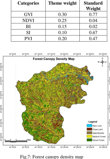
After constructing all the above vegetation indices several weightage values has been considered on its momentous approach using multi criteria analysis method to evaluate the forest canopy density map of the study area. All the raster vegetation indices like GVI, NDVI, BI, SI, and PVI were consigned relevant theme weights and class weights. The individual standard weights are multiplied based on std. Dev. by its respective class score and then all the thematic layers are arranged in a linear permutation equation in Erdas Imagine software. The equation is set up as: Forest Cover Density =
(GVI*0.77+NDVI*0.04+BI*0.02+SI*0.67+PVI*0.47)
Table 1: Gradation & Scoring in each vegetation indices
GVI NDVI BI
Grade Scor
e
Grade Scor
e
Grade Score
Very low 1 Very low 1 Very low 10
Low 1 Low 1 Low 8
Moderate 7 Moderate 1 Moderate 4 High 9 High 9 High 1 Very
high
10 Very high
5 Very high
1
St. Dev. 25.7 8
St. Dev. 0.16 St. Dev. 0.20
Table 2: Evaluate the theme weight and standard weight in support of std. Dev. of scoring
Fig.7: Forest canopy density map
4.7 Accuracy Assessment Report:
Accuracy assessment should be an important component of any categorization. Because it is frequently not done, the reason for this is that it habitually occupies a lot of work in the field, which can be very expensive and time consuming. With the escalating accessibility of Landsat ETM+ images, the developed strategy on an extensive phase similarly will be relevant in several regions of the world. For equipped relevancies of this approach in excess of large areas, we have to need investigation effort for
SI PVI
Grade Score Grade Score
Very low 1 Very low 1
Low 1 Low 1
Moderate 4 Moderate 4
High 9 High 9
Very high 10 Very high 10 St. Dev. 67.45 St. Dev. 67.45
Categories Theme weight Standard
Weight
GVI 0.30 0.77
NDVI 0.25 0.04
BI 0.15 0.02
SI 0.10 0.67
29 the improved precision. How much suspicions decode
to mistakes in the 30 m canopy density data and influence the developed canopy density map. Hence the Multi Criteria Analysis (MCA) operations are the standard methods and its prediction potentiality should supply that which accuracy levels are suitable in categorizes high declaration images. So the accuracy assessment report is indicating as:
Table 3: Accuracy Assessment Report
Overall Accuracy: 86.40% Kappa Coefficient: 79.62%
Producers Accuracy: Results from dividing the
number of correctly classified points for each class (on the major diagonal) by the number of reference points “known” to be of that category (the column total)
User’s Accuracy: computed by dividing the number
of correctly classified points in each class by the total number of points that were classified in that class (the row total)
Overall Accuracy: It is computed by dividing the
total number of correctly classified points (i.e., the sum of the elements along the major diagonal) by the total number of reference points.
Kappa Co-efficient: Measure of agreement between
the classification map and the reference data.
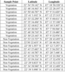
Fig.8: Ground Truthing Point
Table 4: Ground truth sampling point from Google Earth satellite imagery
Category Reference
Classified
producer’s Accuracy
user’s Accuracy
Dense Forest
4 83% 79%
Medium Forest
5 74% 81%
Open/Scrubs 7 87% 89%
Grass Land 8 86% 93%
Bare Land 3 91% 95%
Sample Point Latitude Longitude
30
5. Conclusion:
Conventional RS methodology, as generally applied in forestry is based on qualitative analysis of information derivative from training areas. From exceeding study we terminate that there is the opportunity to demonstrate some empirical operation through Multi Criteria Analysis (MCA) method using Landsat ETM+ data to illustrate the spatial dissimilarity of Species and forest composition. Using the most significant indices for model development may accompany to predict with better capability of vegetation dynamism. Analyzing the behavior of the information in this research we simplify of soaring spatial variation of the forest structure in this area using Landsat ETM+ image. Then we can evidently discriminate between vegetation in the canopy and vegetation on the ground. For the precision of this study some sampling point has been collected from Google Earth imagery to establish the vegetation coverage density on the ground.
Reference:
[1] Boone, R.B., K.A. Galvin, N.M. Smith and S.J. Lynn. 2000. Generalizing El Niño effects upon Maasai livestock using hierarchical clusters of vegetation patterns. Photogrammetric
Engineering & Remote Sensing 66(6): 737-744.
[2] Chen, D. and W. Brutsaert. 1998. Satellite-sensed distribution and spatial patterns of vegetation parameters over a tall grass prairie. Journal of the Atmospheric Sciences 55(7): 1225-1238.
[3] F. Maselli, C. Conese, T. D. Filippis, and S. Norcini, "Estimation of forest parameters through fuzzy classification of TM data," IEEE Transactions on Geoscience and Remote Sensing, Vol. 33, No. 1, pp. 77-84, 1995. [4] Jennings, S.B., Brown, N.D., & Sheil, D., 1999.
Assessing forest canopies and understory illumination: canopy closure, canopy cover and other measures. Forestry 72(1): 59–74.
[5] Oesterheld, M., C.M. Di. Bella and H. Kerdiles. 1998. Relation between NOAA-AVHRR satellite data and stocking rate of rangelands. Ecological Applications 8(1): 207-212.
[6] Peters, A.J., M.D. Eve, E.H. Holt and W.G. Whitford. 1997. Analysis of desert plant community growth patterns with high temporal resolution satellite spectra. Journal of Applied
Ecology 34: 418-432.
[7] Richardson and Wiegand, c.L., 1977. Distinguishing vegetation from soil background information. Photogramm. Eng. remote Sens., 43: 1541-1552.
[8] Ricotta, C., G. Avena, and A.D. Palma. 1999. Mapping and monitoring net primary productivity with AVHRR NDVI time-series:
Statistical equivalence of cumulative vegetation indices.Journal of Photogrammetry and Remote
Sensing 54(5): 325-331.
[9] Saei jamalabad, M., Abkar, A.A., 2000. Vegetation Coverage Canopy Density Monitering, Using Satellite Images. ISPRS Commission VII, 17, Amsterdam, Holland. [10]Tucker, C. J. (1979). Red and photographic
infrared linear combinations for monitoring vegetation. Remote Sensing of Environment, 8, 27−150.