Two-Locus Likelihoods Under Variable Population Size and Fine-Scale Recombination Rate Estimation

| INVESTIGATION

Two-Locus Likelihoods Under Variable Population

Size and Fine-Scale Recombination Rate Estimation

John A. Kamm,*,†,1_{Jeffrey P. Spence,}‡,1_{Jeffrey Chan,}†_{and Yun S. Song*},†,§,_**,2

*Department of Statistics,†Computer Science Division,‡Computational Biology Graduate Group, and§Department of Integrative Biology, University of California, Berkeley, California 94720, and **Departments of Mathematics and Biology, University of Pennsylvania, Philadelphia, Pennsylvania 19104

ABSTRACT Two-locus sampling probabilities have played a central role in devising an efficient composite-likelihood method for estimating fine-scale recombination rates. Due to mathematical and computational challenges, these sampling probabilities are typically computed under the unrealistic assumption of a constant population size, and simulation studies have shown that resulting recombination rate estimates can be severely biased in certain cases of historical population size changes. To alleviate this problem, we develop here new methods to compute the sampling probability for variable population size functions that are piecewise constant. Our main theoretical result, implemented in a new software package called LDpop, is a novel formula for the sampling probability that can be evaluated by numerically exponentiating a large but sparse matrix. This formula can handle moderate sample sizes (n#50) and demographic size histories with a large number of epochs (D$64). In addition, LDpop implements an approximate formula for the sampling probability that is reasonably accurate and scales to hundreds in sample size (n$256). Finally, LDpop includes an importance sampler for the posterior distribution of two-locus genealogies, based on a new result for the optimal proposal distribution in the variable-size setting. Using our methods, we study how a sharp population bottleneck followed by rapid growth affects the correlation between partially linked sites. Then, through an extensive simulation study, we show that accounting for population size changes under such a demographic model leads to substantial improvements infine-scale recombination rate estimation.

KEYWORDScoalescent with recombination; two-locus Moran model; sampling probability; importance sampling

T

HE coalescent with recombination (Griffiths and Marjoram 1997) provides a basic population genetic model for re-combination. For a very small number of loci and a constant population size, the likelihood (or sampling probability) can be computed via a recursion (Golding 1984; Ethier and Griffiths 1990; Hudson 2001) or importance sampling (Fearnhead and Donnelly 2001), allowing for maximum-likelihood and Bayesian estimates of recombination rates (Fearnhead and Donnelly 2001; Hudson 2001; McVean

et al. 2002; Fearnheadet al. 2004; Fearnhead and Smith

2005; Fearnhead 2006).

Jenkins and Song (2009, 2010) recently introduced a new framework based on asymptotic series (in inverse powers of the recombination rate r) to approximate the two-locus

sampling probability under a constant population size and developed an algorithm for finding the expansion to an arbitrary order (Jenkins and Song 2012). They also proved that only afinite number of terms in the expansion are needed to obtain theexacttwo-locus sampling probability as an ana-lytic function ofr. Bhaskar and Song (2012) partially extended this approach to an arbitrary number of loci and found closed-form closed-formulas for thefirst two terms in an asymptotic expan-sion of the multilocus sampling distribution.

When there are more than a handful of loci, computing the sampling probability becomes intractable. A popular and tractable alternative has been to construct composite likeli-hoods by multiplying the two-locus likelilikeli-hoods for pairs of SNPs; this pairwise composite likelihood has been used to estimate fine-scale recombination rates in humans (International HapMap Consortium 2007; 1000 Genomes Project Consortium 2010), Drosophila (Chan et al. 2012), chimpanzees (Auton et al. 2012), microbes (Johnson and Slatkin 2009), dogs (Autonet al.2013), and more and was used in the discovery of a DNA motif associated with Copyright © 2016 by the Genetics Society of America

doi: 10.1534/genetics.115.184820

Manuscript received November 13, 2015; accepted for publication May 6, 2016; published Early Online May 9, 2016.

1_{These authors contributed equally to this work.}

2_{Corresponding author: Department of Statistics, 321 Evans Hall # 3860, University of}

recombination hotspots in some organisms, including hu-mans (Myerset al.2008), subsequently identified as a bind-ing site of the protein PRDM9 (Baudatet al.2010; Berget al.

2010; Myerset al.2010).

The pairwise composite likelihood wasfirst suggested by Hudson (2001). The software package LDhat (McVeanet al.

2004; Auton and McVean 2007) implemented the pairwise composite likelihood and embedded it within a Bayesian MCMC algorithm for inference. Chanet al.(2012) modified this algorithm in their program LDhelmet to efficiently utilize the aforementioned asymptotic formulas for the sampling probability, among other improvements. The program LDhot (Myers et al. 2005; Autonet al.2014) uses the composite likelihood as a test statistic to detect recombination hotspots, in conjunction with coalescent simulation to determine ap-propriate null distributions.

Because of mathematical and computational challenges, LDhat, LDhelmet, and LDhot all assume a constant population size model to compute the two-locus sampling probabilities. This is an unrealistic assumption, and it would be desirable to account for known demographic events, such as bottlenecks or popula-tion growth. Previous studies (McVeanet al.2002; Smith and Fearnhead 2005; Chanet al.2012) have shown that incorrectly assuming constant population size can lead these composite-likelihood methods to produce biased estimates. Furthermore, Johnston and Cutler (2012) observed that a sharp bottleneck followed by rapid growth can lead LDhat to infer spurious re-combination hotspots if it assumes a constant population size.

Hudson (2001) proposed Monte Carlo computation of two-locus likelihoods by simulating genealogies. While this generalizes to arbitrarily complex demographies, it would be desirable to have a deterministic formula, as naive Monte Carlo computation sometimes has difficulty approximating small probabilities.

In this article, we show how to compute the two-locus sampling probability exactly under variable population size histories that are piecewise constant. Our approach relies on the Moran model (Moran 1958; Ethier and Kurtz 1993; Donnelly and Kurtz 1999), a stochastic process closely related to the coalescent. We have implemented our results in a freely available software package, LDpop, that efficiently produces lookup tables of two-locus likelihoods under variable population size. These lookup tables can then be used by other programs that use composite likelihoods to infer recombination maps.

Our main result is an exact formula, introduced inTheorem 1, that involves exponentiating sparsem3mmatrices con-tainingOðmÞnonzero entries, wherem¼Oðn6_{Þunder a}

bial-lelic model, with n being the sample size. We derive this formula by constructing a Moran-like process in which sam-ple paths can be cousam-pled with the two-locus coalescent and by applying a reversibility argument.

Theorem 1has a high computational cost, and our

imple-mentation in LDpop can practically handle low to moderate sample sizes (n,50) on a 24-core compute server. We have thus implemented an approximate formula that is much faster and scales to sample sizes in the hundreds. This

formula is computed by exponentiating a sparse matrix with

Oðn3_{Þnonzero entries and is based on a previous two-locus}

Moran process (Ethier and Kurtz 1993), which we have implemented and extended to the case of variable population size. While this formula does not give the exact likelihood, it provides a reasonable approximation and converges to the true value in an appropriate limit.

In addition to these exact and approximate formulas, LDpop also includes a highly efficient importance sampler for the posterior distribution of two-locus genealogies. This can be used to infer the genealogy at a pair of sites and also provides an alternative method for computing two-locus likelihoods. Our importance sampler is based on an optimal proposal distribution that we characterize in Theorem 2. It generalizes previous results for the constant-size case, which have been used to construct importance samplers for both the single-population, two-locus case (Fearnhead and Donnelly 2001; Dialdestoroet al.2016) and other constant-demography coalescent scenarios (Stephens and Donnelly 2000; De Iorio and Griffiths 2004; Griffithset al.2008; Hobolthet al.2008; Jenkins 2012; Koskelaet al.2015). The key ideas ofTheorem 2

should similarly generalize to other contexts of importance sampling a time-inhomogeneous coalescent.

Using a simulation study, we show that using LDpop to ac-count for demography substantially improves the composite-likelihood inference of recombination maps. We also use LDpop to gain a qualitative understanding of linkage disequi-librium by examining ther2_{statistic. Finally, we examine how}

LDpop scales in terms of sample sizenand the numberDof demographic epochs. The exact formula can handlenin the tens, while the approximate formula can handle n in the hundreds. Additionally, we find that the runtime of LDpop is not very sensitive toD;so LDpop can handle size histories with a large number of pieces.

LDpop is freely available for download athttps://github. com/popgenmethods/ldpop.

Background

Here we describe our notational convention and review some key concepts regarding the coalescent with recombination and the two-locus Moran model.

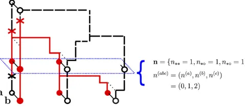
Figure 1 An ancestral recombination graph (ARG) at two loci, labeled

“a”and“b”, each with two alleles (•and∘). The notationsn;nij;nðabcÞare

Notation

Let u=2 denote the mutation rate per locus per unit time,

P¼ ðPijÞi;j2A be the transition probabilities between alleles

given a mutation, andA ¼ f0;1gbe the set of alleles (our formulas can be generalized tojAj.2;but this increases the computational complexity). Let r=2 denote the recombi-nation rate per unit time. We consider a single panmictic population, with piecewise-constant effective population sizes. In particular, we assume D pieces, with end-points2N¼t2D,t2Dþ1,⋯,t21,t0¼0;where 0

corre-sponds to the present andt,0 corresponds to a time in the past. The pieceðtd;tdþ1is assumed to have scaled population

sizehd:Going backward in time, two lineages coalesce (find a

common ancestor) at rate 1=hdwithin the intervalðtd;tdþ1:

We allow the haplotypes to have missing (unobserved) alleles at each locus and use * to denote such alleles. We denote each haplotype as having type a, b, or c, where a

haplotypes are observed only at the left locus,bhaplotypes are observed only at the right locus, and c haplotypes are observed at both loci. Overloading notation, we sometimes refer to the left locus as thealocus and the right locus as theb

locus. We usen¼ fni_*;n_*j;nkℓgi;j;k;ℓ2Ato denote the confi

gu-ration of an unordered collection of two-locus haplotypes, with ni* denoting the number of a types with allele i, n*j

denoting the number ofbtypes with allelej, andnkℓdenoting the number ofctypes with alleleskandℓ:

Suppose nhasnðabcÞ_{¼ ðn}ðaÞ_;nðbÞ_;nðcÞ_{Þ haplotypes of type} a;b;c;respectively. We define thesampling probabilityℙtðnÞ

to be the probability of samplingnat timet, given that we observed nðaÞ_;nðbÞ_;nðcÞ _{haplotypes of type a;b;c;under the}

coalescent with recombination (described below).

The ancestral recombination graph and the coalescent with recombination

The ancestral recombination graph (ARG) is the multilocus genealogy relating a sample (Figure 1). The coalescent with recombination (Griffiths 1991) gives the limiting dis-tribution of the ARG under a wide class of population models, including the Wright–Fisher model and the Moran model.

LetnðtcÞbe the number of lineages at timetthat are

ances-tral to the observed present-day sample at both loci. Similarly, letnðtaÞandn

ðbÞ

t be the number of lineages that are ancestral at

only theaorblocus, respectively. Under the coalescent with recombination, nðtabcÞ¼ ðnð

aÞ t ;nð

bÞ t ;nð

cÞ

t Þ is a backward-in-time

Markov chain, where eachc-type lineage splits (recombines) into onea and oneblineage at rater=2;and each pair of lineages coalesces at rate 1=hd within the time interval

ðtd;tdþ1:Table 1 gives the transition rates ofnðtabcÞ:

After sampling the history of coalescence and recombina-tion eventsfnðtabcÞgt#0;we drop mutations down at rateu=2

per locus, with alleles mutating according toP;and the alleles of the common ancestor assumed to be at the stationary dis-tribution. This gives us a sample pathfntgt#0;wheren0is the

observed sample at the present, and nt is the collection of ancestral haplotypes at timet. Under this notation, the sam-pling probability at timetis defined as

ℙtðnÞ:¼ℙ

nt¼njnðabcÞt ¼nðabcÞ

: (1)

Two-locus Moran model

The Moran model is a stochastic process closely related to the coalescent and plays a central role in our results. Here, we review a two-locus Moran model with recombination dynam-ics from Ethier and Kurtz (1993). We note that there are multiple versions of the two-locus Moran model, and in par-ticular Donnelly and Kurtz (1999) describe a Moran model with different recombination dynamics.

Table 1 Backward-in-time transition rates ofnðabcÞt ¼ ðn ðaÞ t ;n

ðbÞ t ;n

ðcÞ t Þ within time interval ðtd;tdþ1 under the coalescent with recombination

End state Rate

nðtaÞþ1;n ðbÞ t þ1;n

ðcÞ

t 21 r2n

ðcÞ t

nðtaÞ21;n ðbÞ t ;n

ðcÞ t

1 h_dn

ðaÞ t

nðtaÞ21

2 þn

ðcÞ t

nðtaÞ;n ðbÞ t 21;n

ðcÞ t

1 h_dn

ðbÞ t

nðtbÞ21

2 þn

ðcÞ t

nðtaÞ;n ðbÞ t ;n

ðcÞ t 21

1 h_d

nðtcÞ

2

nðtaÞ21;n ðbÞ t 21;n

ðcÞ t þ1

1 h_dn

ðaÞ t n

ðbÞ t

The Moran model withNlineages is afinite population model evolving forward in time. In particular, letMtdenote a collection ofNtwo-locus haplotypes at timet(with no miss-ing alleles). ThenMtis a Markov chain going forward in time that changes due to mutation, recombination, and copying events.

Let Ld_ðNÞ denote the transition matrix of Mt within ðtd;tdþ1: We describe the rates of Ld_ðNÞ: For the mutation

events, each allele mutates at rateu=2 according to transition matrixP:For the copying events, each lineage ofMtcopies its haplotype onto each other lineage at rate 1=2hdwithin the

time interval ðtd;tdþ1: Biologically, this corresponds to

one lineage dying out and being replaced by the offspring of another lineage, which occurs more frequently when genetic drift is high (i.e., when the population size hd

is small). Finally, every pair of lineages in Mt swaps genetic material through a crossover recombination at rate r=2ðN21Þ: A crossover between haplotypes ði1;j1Þ

and ði2;j2Þ results in new haplotypes ði1;j2Þ and ði2;j1Þ;

and the configuration resulting from the crossover is

Mt2ei1;j12ei2;j2þei1;j2þei2;j1:See Figure 2 for illustration. LetℙðtNÞðnÞbe the probability of samplingnat timetunder

this Moran model, for a configuration nwith sample size

n#N: ℙðtNÞðnÞ is given by first sampling Mminðt;t2Dþ1Þ from the stationary distribution l2_ðNDÞ of L2ðNDÞ; then propagating fMsgs#0forward in time tot, and then samplingnwithout

replacement fromMt:So,

h

ℙðNÞðMt¼MÞ i

M¼l

2D ðNÞ

Y21

d¼2Dþ1

eLdðNÞ½minðt;tdþ1Þ2minðt;tdÞ

ℙðNÞt ðnÞ ¼ X

M

 ℙðNÞðMt¼MÞℙðnjMÞ;

(2)

whereℙðnjMÞdenotes the probability of samplingnwithout replacement fromM;and½ℙðNÞðMt¼MÞMandl2ðNDÞare row

vectors here.

In general,ℙðtNÞðnÞ 6¼ℙtðnÞ;soMtdisagrees with the

co-alescent with recombination. However, the likelihood under

Mtconverges to the correct value,ℙðtNÞðnÞ/ℙtðnÞasN/N:

In fact, even forN¼n¼20;wefind thatℙðtNÞðnÞprovides a

reasonable approximation for practical purposes (see

Fine-scale recombination rate estimation and Accuracy of the

approximate likelihood). We refer to (2),i.e., the likelihood under Mt;as the “approximate-likelihood formula,”in con-trast to the exact formula we present inTheorem 1below. This approximate formula is included in LDpop as a faster, more scalable alternative to the exact formula ofTheorem 1.

Data availability

The authors state that all data necessary for confirming the conclusions presented in the article are represented fully within the article. Scripts to reproduce the simulated data analysis are available from the authors on request.

Theoretical Results

In this section, we describe our theoretical results. Proofs are deferred to theAppendix.

Exact formula for the sampling probability

Our main result is an explicit formula for the sampling prob-abilityℙðnÞ;presented inTheorem 1. We present an outline here; the proof is shown in theAppendix.

The idea is to construct a forward-in-time Markov process Mt~ and relate its distribution to the coalescent with recombination. Mt~ is similar to the Moran model

Mt described above, except thatMt~ allows partially spec-ified a and b types, whereas all lineages in Mt are fully specified c types. Specifically, the state space of Mt~ is

N ¼ fn:nðabcÞ_{¼ ðk;k;n2kÞ;0#k#ng the collection of}

sample configurations withnspecified (nonmissing) alleles at each locus. The state ofMt~ changes due to copying, muta-tion, recombinamuta-tion, and “recoalescence” events. Copying and mutation dynamics are similar toMt;but recombination is different: everyctype splits intoaandbtypes at rater=2; and every pair ofaandbtypes“recoalesces”back into actype at rate 1=hd:An illustration is shown in Figure 3B;Mt~ is

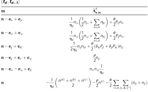
de-scribed in more detail in the Appendix. Within interval

ðtd;tdþ1;we denote the transition rate matrix ofMt~ asL~

d

;

a square matrix indexed byN;with entries given in Table 2. ~

Mt does not itself yield the correct sampling probability. The basic issue is that Mt~ hasctypes splitting intoaandb

types at rate r=2 going forward in time, but under the co-alescent with recombination, this needs to happen at rate r=2 goingbackward in time. Similarly, pairs ofaandbtypes merge into a singlectype at rate 1=hdgoing forward in time

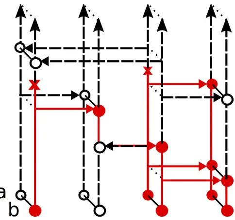
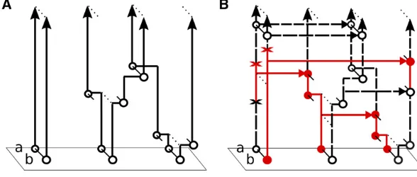
Figure 3The process fM~tgt#0 with ratesL~ d

(Table 2) used to proveTheorem 1. This process is similar tofMtg

(Figure 2), in thatnis fixed, and alleles change due to copying and mutation. However,M~tallows partially

spec-ifiedaandbtypes, withctypes recombining into a pair of aandbtypes, and pairs ofaandbtypes recoalescing into c types. (A) The processfCtgt#0 of just recombination

(c/a;b) and recoalescence (a;b/c) events. (B) The full processfM~tgt#0including copying, mutation,

underMt~ ;but going backward in time under the coalescent with recombination.

However, it is possible to “reverse” the direction of the recombinations (c/a;b) and recoalescences (a;b/c), to get a new process that does match the two-locus coalescent. In particular, letCtbe the number of c

types inMt~ ;illustrated in Figure 3A. ThenCtis a

revers-ible Markov chain, whose rate matrix in ðtd;tdþ1isGd;a

tridiagonal square matrix indexed by f0;1;. . .;ng; with Gd

m;m21¼ ðr=2Þm; G

d

m;mþ1 ¼ ðn2mÞ 2_ð

1=hdÞ; and G d m;m¼

2Gd

m;m212G

d

m;mþ1:Exploiting the reversibility ofCt allows

us to relate the distribution of Mt~ to the coalescent with recombination and obtain the following result:

Theorem 1.Letðgd

0;. . .;gdnÞbe the stationary distribution

ofGd;and let the row vector~gdbe indexed byN;withg~d_n¼gd m

if nhas m lineages of type c.Denote the stationary

distribu-tion ofL~dby the row vectorL~d¼ ðld_nÞ_n2N:Let⊙andO de-note component-wise multiplication and division,and recursively define the row vectorpd_{¼ ðp}d

nÞn2N by

p2Dþ1_¼l~2D_Og~2D pdþ1_{¼ ½ðp}d_⊙~gd_ÞeL~d

ðtdþ12tdÞOg~d:

(3)

Then,forn2 N;we haveℙ0ðnÞ ¼p0n:

Note thatTheorem 1givesℙ0ðnÞforn2 N:This includes

all fully specifiedn;i.e., withnðabcÞ_{¼ ð0;0;nÞ;and suffices for}

the application considered in Fine-scale recombination rate estimation. If necessary, ℙ0ðnÞ for partially specified n can

be computed by summing over the fully specified confi gura-tions consistent withn:

For jAj ¼2 alleles per locus, L~d is an Oðn6_Þ3Oðn6_Þ

matrix, so naively computing the matrix multiplication

in Theorem 1 would cost Oðn12_{Þ time. However, L}~d _is

sparse, with Oðn6_{Þ nonzero entries, allowing efficient}

algorithms to compute Theorem 1(up to numerical preci-sion) in Oðn6_{T Þtime, where T is some finite number of}

matrix–vector multiplications. See the Appendix for more details.

Importance sampling

In addition to the approximate (Equation 2) and exact (Equa-tion 3) formulas for the sampling probability, LDpop includes an importance sampler for the two-locus ARGn#0¼ fntgt#0:

This provides a method to sample from the posterior distri-bution of two-locus ARGs and also provides an alternative method for computing ℙ0ðnÞ: This importance sampler is

based onTheorem 2below, which characterizes the optimal proposal distribution for the two-locus coalescent with re-combination under variable population size.

Let the proposal distributionQðn#0Þbe a probability

dis-tribution onfn#0:n0¼ngwhose support contains that of

ℙðn_#0jn0¼nÞ:Then we have

ℙ0ðnÞ ¼ Z

n#0:n0¼n

dℙðn#0Þ dQðn_#0Þ 

dQðn_#0Þ;

and so, ifnð_#1Þ₀;. . .;nð_#KÞ₀ Qi.i.d., the sum

1 K XK k¼1 dℙ nðkÞ_#0

dQnðkÞ_#0 (4)

converges almost surely toℙ0ðnÞasK/Nby the law of large

numbers. Hence, (4) provides a Monte Carlo approximation to ℙ0ðnÞ:The optimal proposal is the posterior distribution

Qoptðn#0Þ ¼ℙðn#0jn0Þ;for then (4) is exactly

1 K XK k¼1 dℙ nðkÞ_#0

dℙ

nðkÞ_#0n0

¼1 K XK k¼1 dℙ nðkÞ_#0

dℙnðkÞ_#0.ℙðn0Þ

¼ℙðn0Þ;

even forK¼1.

The following theorem, which we prove in theAppendix, characterizes the optimal posterior distributionQoptðn#0Þ ¼

ℙðn#0jn0Þfor variable population size:

Theorem 2. The process fntgt#0 is a backward-in-time

Markov chain with inhomogeneous rates,whose rate matrix

at time t is given by

qðtÞn;m¼

fðtÞn;mℙtðmÞ

ℙtðnÞ; if

m6¼n;

fðtÞn;n2d

dtlogℙtðnÞ; if m¼n; 8 > > < > > :

wherefðtÞ¼ ðf_nðt_;Þ_mÞis a square matrix,indexed by

configura-tionsn;with entries given by Table3and equal to

fðtÞn;m¼ d ds

h

ℙnðabcÞ_t2s ¼mðabcÞnðabcÞ_t ¼nðabcÞ

3 ℙnt¼njnt2s¼m;nðabcÞt ¼nðabcÞi_s¼ 0:

(5)

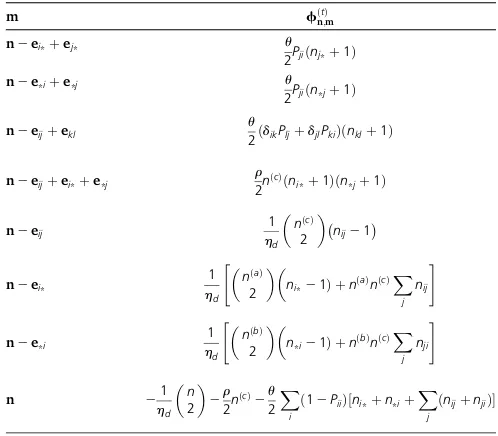
Intuitively, the matrixfðtÞin Table 3 is a linear combina-tion of two rate matrices, one for propagating nðtabcÞ an Table 2 Nonzero entries of the rate matrix L~d for the interval

ðtd;tdþ1

m L~d_n;m

n2ei*þej* 1

h_dni* ₁

2nj*þ X

k2A njk

þu

2Pijni*

n2e_*iþe*j 1

h_dn*i

1 2n*jþ

X

k2A nkj

þu

2Pijn*i

n2eijþekl

1 2h_dnijnklþ

u

2ðdikPjlþdjlPikÞnij

n2eijþei*þe*j

r

2nij

n2e_i*2e_*jþe_{ij ni*n*j}1

h_d

n 2_h1

d

nðaÞ_þnðbÞ_þnðcÞ

2

2r₂nðcÞ₂u

2 X

i2A

X

infinitesimal distance backward in time and another for prop-agatingnt an infinitesimal distance forward in time. This is because nðtabcÞ is generated by sampling coalescent and

re-combination events backward in time, and thenntis gener-ated by dropping mutations on the ARG and propagating the allele values forward in time.

Theorem 2 generalizes previous results for the optimal

proposal distribution in the constant-size case (Stephens and Donnelly 2000; Fearnhead and Donnelly 2001). In that case, the conditional probability of the parent m of nis f_n;mðℙðmÞ=ℙðnÞÞ:Note the constant-size case is time homo-geneous, so the dependence ontis dropped, and the waiting times between events in the ARG are not sampled (i.e., only the embedded jump chain ofn#0is sampled).

We construct our proposal distribution Qð^ n#0Þ by

ap-proximating the optimal proposal distributionQoptðn#0Þ ¼

ℙðn#0jn0Þ: This requires approximating the rate qðnt;Þm¼ fð_nt_;Þ_mðℙtðmÞ=ℙtðnÞÞ: We use the approximation ^qðnt;Þm¼ fð_nt_;Þ_mðℙðtNÞðmÞ=ℙ

ðNÞ

t ðnÞÞ;withℙ ðNÞ

t ðnÞfrom the

approximate-likelihood Equation 2. To save computation, we compute

ℙðNÞ

t ðnÞonly along a grid of time points and then linearly

interpolate^qð_nt_;Þ_mbetween the points. See theAppendixfor more details on our proposal distributionQ:^

As detailed in Runtime and accuracy of the importance sampler,Q^is a highly efficient proposal distribution, typically yielding effective sample sizes (ESS) between 80% and 100% per sample for the demography andrvalues we considered.

Application

Previous simulation studies (McVeanet al.2002; Smith and Fearnhead 2005; Chanet al.2012) have shown that if the

demographic model is misspecified, composite-likelihood methods (which so far have assumed a constant population size) can produce recombination rate estimates that are biased. Many populations, including those of humans and

Drosophila melanogaster, have undergone bottlenecks and

expansions in the recent past (Choudhary and Singh 1987; Gutenkunstet al. 2009), and it has been argued (Johnston and Cutler 2012) that such demographies can severely affect recombination rate estimation and can cause the appearance of spurious recombination hotspots.

In this section, we apply our software LDpop to show that accounting for demography improvesfine-scale recombination rate estimation. Wefirst examine how a population bottleneck followed by rapid growth affects the correlation between partially linked sites. We then study composite-likelihood esti-mation of recombination maps under a population bottleneck. Wefind that accounting for demography with either the exact

(Theorem 1)- or approximate (Equation 2)-likelihood formula

substantially improves accuracy. Furthermore, this improve-ment is robust to minor misspecification of the demography due to not knowing the true demography in practice.

Throughout this section, we use an example demography with D¼3 epochs, consisting of a sharp population bottle-neck followed by a rapid expansion. Specifically, the popula-tion size historyhðtÞ;in coalescent-scaled units, is given by

hðtÞ ¼

8 < :

100; 20:5,t#0; 0:1; 20:58,t#20:5; 1; t#20:58:

(6)

Under this model and n¼2; the expected time of the common ancestor is E½TMRCA 1: We thus compare this

demography against a constant-size demography with coalescent-scaled size of h[1;as this is the population size that would be estimated using the pairwise heterozygos-ity (Tajima 1983). We use a coalescent-scaled mutation rate ofu=2¼0:004 per base, which is roughly the mutation rate

ofD. melanogaster(Chanet al.2012).

While the size historyhðtÞof (6) is fairly simple, with only

D ¼3 epochs, we stress that LDpop can in fact handle much more complex size histories. For example, inRuntime and

Accu-racy of Likelihoods, we show that LDpop can easily handle a

demography withD ¼64;with little additional cost in runtime.

Linkage disequilibrium and two-locus likelihoods

One statistic of linkage disequilibrium is

^r2¼ h

^

x112^xðaÞ1 ^x ðbÞ 1

i2

^

xðaÞ₀ ^xðaÞ₁ ^xðbÞ₀ ^xðbÞ₁ ;

where^xij¼nij=nis the fraction of the sample with haplotype

ij;with^xð_iaÞ¼P_j^xijand^xð bÞ j ¼

P

i^xij:In words,^r2is the

sam-ple square correlation of a random allele at locus awith a random allele at locusb. We letr2_¼lim

n/N^r2 denote the population square correlation. There has been considerable

Table 3 Nonzero entries of the fðtÞ matrix of Theorem 2, for t2 ðtd;tdþ1

m fðtÞ

n;m

n2ei*þej* u

2Pjiðnj*þ1Þ

n2e_*iþe*j u

2Pjiðn*jþ1Þ

n2eijþekl

u

2ðdikPljþdjlPkiÞðnklþ1Þ

n2eijþei*þe*j

r

2n

ðcÞ_ðn

i*þ1Þðn*jþ1Þ

n2e_ij 1

h_d

nðcÞ

2

nij21

n2ei*

1

h_d

"

nðaÞ

2

ni*21Þ þn

ðaÞ nðcÞX

j nij

#

n2e_*i

1

h_d

"

nðbÞ

2

n*i21Þ þnðbÞnðcÞ

X

j nji

#

n 2_h1

d n 2 2r 2n

ðcÞ₂u

2 X

i

ð12PiiÞ½ni*þn*iþ

X

theoretical interest in understanding moments ofr2_;^r2_;

and related statistics (Ohta and Kimura 1969; Maruyama 1982; Hudson 1985; McVean 2002; Song and Song 2007). Addi-tionally, n^r2 approximately follows a x2

1 distribution when

r2_{¼0;which provides a test for the statistical significance}

of linkage disequilibrium (Weir 1996, p. 113).

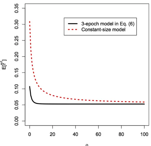
Using LDpop, we can compute the distribution of^r2 for piecewise constant models. In Figure 4, we showE½^r2for a sample sizen¼20 under the three-epoch model (6) and the constant population size model. Under the three-epoch de-mography,E½^r2is much lower for smallrand decays more rapidly asr/N:In other words, the constant model requires higher r to break down linkage disequilibrium (LD) to the same level, which suggests that incorrectly assuming a con-stant demography will lead to upward-biased estimates of the recombination rate (as pointed out by an anonymous reviewer). We confirm this below.

Fine-scale recombination rate estimation

For a sample ofnhaplotypes observed atLSNPs, letn½a;bbe the two-locus sample observed at SNPsa;b2 f1;. . .;Lg;and letr½a;bbe the recombination rate between SNPsaandb. The programs LDhat (McVeanet al.2002, 2004; Auton and McVean 2007), LDhot (Myerset al.2005; Autonet al.2014), and LDhelmet (Chanet al.2012) infer hotspots and recom-bination maps r; using the composite likelihood due to Hudson (2001),

Y

a;b: 0,b2a,W

ℙn½a;b;r½a;b; (7)

where W denotes some window size in which to consider pairs of sites [afinite window sizeWremoves the computa-tional burden and statistical noise from distant, uninforma-tive sites (Fearnhead 2003; Smith and Fearnhead 2005)].

We used LDpop to generate four likelihood tables, which we then used with LDhat and LDhelmet to estimate recom-bination maps for simulated data. The four tables, denoted by

Lconst;Lexact;Lapprox;andLmiss;are defined as follows:

1. (“Constant”) Lconst denotes a likelihood table that

as-sumes a constant population size ofh[1:

2. (“Exact”) Lexact denotes a likelihood table that assumes

the correct three-epoch population size historyhdefined in (6).

3. (“Approximate”) Lapprox denotes a likelihood table with

the correct size history h in (6), but using the (much faster) approximate-likelihood Equation 2 with N¼n

Moran particles.

4. (“Misspecified”)Lmissdenotes a likelihood table that

as-sumes a misspecified demographyh^;defined by

^ hðtÞ ¼

8 < :

90:5; 20:534,t#0; 0:167; 20:66,t#20:534;

1:0; t#20:66;

(8)

which was estimated from simulated data (Appendix)

Overall, we found that using the constant tableLconstleads to

very noisy and biased estimates ofr(as might be expected from Figure 4). The other tablesLexact;Lapprox;andLmissall lead to

much more accurate estimates. UsingLexact(the exact-likelihood

table with the true size history) produces slightly more accurate estimates ofrthan usingLapprox orLmiss:However, the three

nonconstant tables Lexact; Lapprox; and Lmiss all produce very

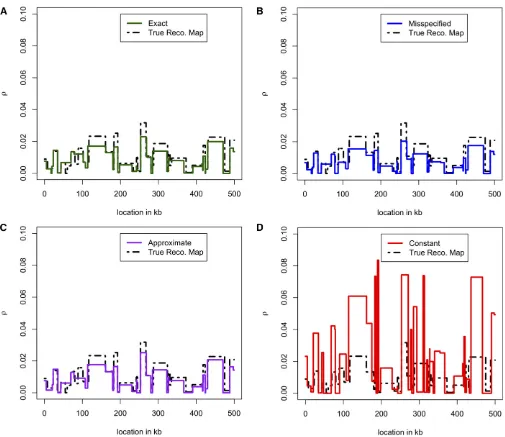
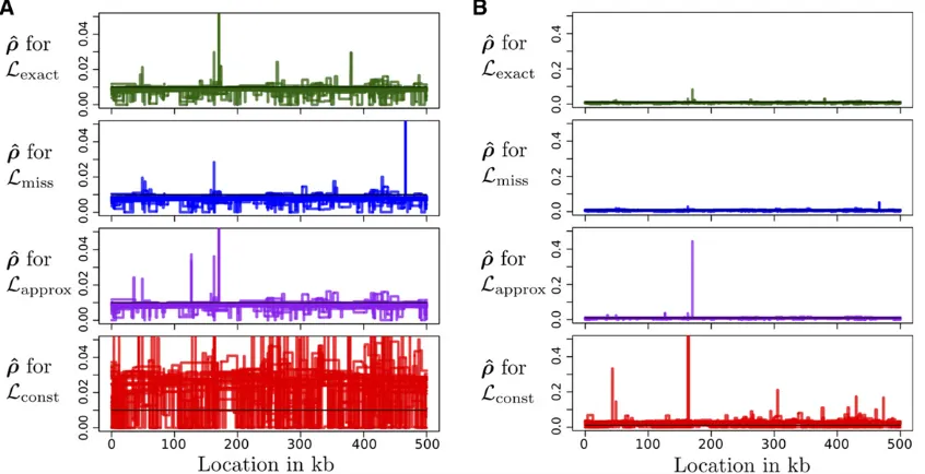
similar results that are hard to distinguish from one another. Figure 5 and Figure 6 show the accuracy of estimated re-combination maps^ron simulated data. We simulatedn¼20 sequences under the three-epoch demography defined in (6), with the true mapsrtaken from previous estimates for the X chromosome of D. melanogaster(Chanet al. 2012). In all, there were 110 independent data sets, with estimated maps ^

rof length 500 kb. See theAppendixfor further details. In Figure 5, we plotrand^rfor a particular 500-kb region. Qualitatively, the constant-size estimate^r_Lconst is less accurate and has wilder fluctuations. Figure 6 shows that over all 110 replicates, the constant-size estimate^rLconst has high bias and low correlation with the truth, compared to the estimates ^

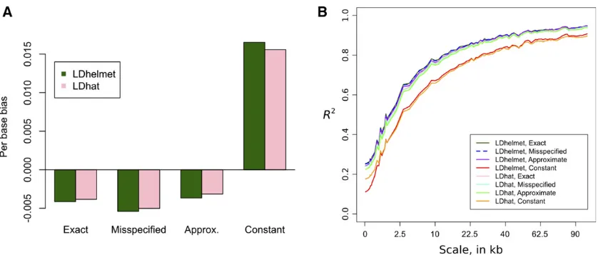
r_Lexact;r^_Lmiss;and^rLapproxthat account for variable demography. Following Wegmannet al.(2011), we plot the correlation of r^ withr at multiple scales; at all scales, the constant-demography estimate^rLconstis considerably worse than the other estimates. In general, using an inferred demography or an approximate lookup table results in only a very mild reduction in accuracy compared to using the true sampling probabilities. We also considered a constant (flat) mapr;the estimatedr^ are shown in Figure 7. Consistent with Johnston and Cutler

(2012), we find that the constant-demography estimate ^

r_Lconst can have extreme peaks and is generally very noisy. On the other hand, the estimates ^rLexact; r^Lmiss; r^Lapprox that account for demography have less noise and fewer large deviations.

Runtime and Accuracy of Likelihoods

Runtime of the exact and approximate-likelihood formulas

Both the approximate (Equation 2)- and exact-likelihood formulas (Theorem 1) require computing products veA for

somek3kmatrixAand 13krow vectorv:Naively, this kind of vector–matrix multiplication costsOðk2_{Þ:However, in our}

caseA is sparse, with OðkÞ nonzero entries, allowing us to computeveAup to numerical precision inOðkT Þtime, where

T is some finite number of sparse matrix–vector products depending onA(Al-Mohy and Higham 2011). In particular,

k¼Oðn3_{Þfor the approximate formula, whereask¼Oðn}6_Þ

for the exact formula. Thus, computing the likelihood table costsOðn3_{T ÞandOðn}6_{T Þfor the approximate (Equation 2)}

and exact (Theorem 1) formulas, respectively. See the Appen-dix for a more detailed analysis of the computational com-plexity and a description of the algorithm for computingveA:

Figure 5 Comparison of recombination maps inferred using different lookup tables. We simulatedn¼20 haplotypes under the three-epoch model (6) and using the recombination map shown as a black dashed line. (A) Inferred mapr^Lexactobtained using the exact likelihoods for the true demography. (B) Inferred map^rLmissobtained using the empirically estimated demography in (8). (C) Inferred mapr^Lapproxobtained using an approximate lookup table

for the true demography. (D) Inferred map^rLconstobtained assuming a constant population size ofh[1:Note that^rLconstis much noisier than the other

Note thatT depends nontrivially on the sample sizen, as well as the parametersr,u,hd;andtd:

We present running times for LDpop in Figure 8. We used LDpop to generate likelihood tables withr2 f0;1;. . .;100g; using 24 cores on a computer with 256 GB of RAM. On the three-epoch demography (Equation 6), we ran the exact for-mula up ton¼40 (17 hr) and the approximate formula up to

n¼256 (13 hr). The constant demography takes nearly the same amount of time as the three-epoch demography, which agrees with our general experience that computing the initial stationary distributionl~2Dis more expensive than multiplying the matrix exponentials eL~dt_{:Using faster}

algo-rithms to computel~2D should lead to substantial improve-ments in runtime.

Figure 8 also examines how LDpop scales with the number of epochs in the demography. We split½2Tmax;0intoD

in-tervals of lengthTmax=D;each with a random population size

1=hdlog Uniformð0:1;10Þ;with 10 repetitions per setting

ofTmaxandD:Empirically, LDpop scales sublinearly withD;

and LDpop has no problem handlingD ¼64 epochs. We also note thatTmaxhas a greater impact on runtime thanD;this is

because the matrix exponentials are essentially computed by solving an ordinary differential equation (ODE) from2Tmax

to 0, as noted in theAppendix; seeComputing the action of a sparse matrix exponential.

Accuracy of the approximate likelihood

In the Fine-scale recombination rate estimation section, we found that using the approximate likelihood (Equation 2) has little impact on recombination rate estimation, suggest-ing that it is an accurate approximation to the exact formula

inTheorem 1. We examine this in greater detail in Figure 9,

for n¼20;the three-epoch demography (Equation 6), and a lookup table with r2 f0;1;. . .;100g We compare the approximate against the exact values forN¼20 andN¼100

Moran particles in the approximate model. The approximate table with N¼20 is reasonably accurate, with some mild deviations from the truth. The approximate table with

N¼100 is extremely accurate and visually indistinguishable from the true values.

Runtime and accuracy of the importance sampler

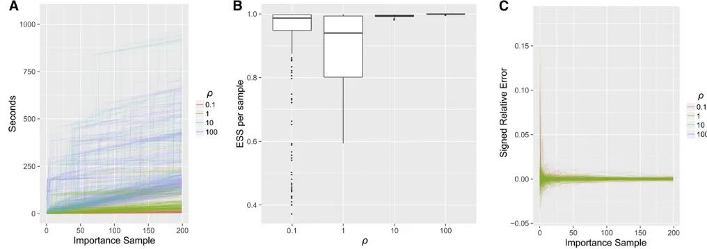
We plot the runtime of our importance sampler in Figure 10A. For the previous three-epoch demography (Equation 6), we drewK¼200 importance samples for each of the 275 confi g-urationsnwithn¼nðcÞ_{¼20;withr2 f0:1;1;10;100gThe}

runtime of the importance sampler generally increased with r; using 20 cores, sampling all 275 configurations took

4 min withr¼0:1;but about 1 hr withr¼100:We fur-ther analyze the computational complexity of the importance sampler in theAppendix.

The numberKof importance samples required to reach a desired level of accuracy is typically measured with ESS,

ESS¼

X_​K

k¼1wk 2

X_​K k¼1w

2 k

;

where wk¼dℙðnð_#kÞ0Þ=dQð^ n

ðkÞ

#0Þ denotes the importance

weight of the kth sample (see Equation 4). Note that ESS#Kalways, with equality achieved only if thewkhave

0 variance.

Compared to previous coalescent importance samplers, our proposal distribution is highly efficient. We plot the ESS per importance sample (i.e., ESS=K) in Figure 10B. Typ-ically ESS=K.0:8;forr2 f10;100g;the ESS is close to its optimal value, with ESS=K1:In Figure 10C, we compare the log-likelihood estimated from importance sampling to the true value computed with Theorem 1; after K¼200

Figure 6 Accuracy of the estimated maps^rLexact;^rLmiss;^rLapprox;^rLconst over 110 simulations similar to Figure 5. The estimate^rLconst obtained assuming

constant demography is substantially more biased and noisier than the other estimates. (A) The average per-base bias^r2r:(B) The square Pearson correlation coefficientR2_{over different scales. ThisR}2_{is distinct from ther}2_{statistic measuring linkage disequilibrium. To computeR}2_{for scales, the}

importance samples, the signed relative error is well under 1% for alln:

By contrast, the previous two-locus importance sampler of Fearnhead and Donnelly (2001), which assumes a constant population size, achieves ESS anywhere between 0:05Kand 0:5K;depending onn;u;r (result not shown). This impor-tance sampler is based on a similar result to that ofTheorem 2, with optimal ratesfn;mðℙðmÞ=ℙðnÞÞ:However, to approx-imateℙðmÞ=ℙðnÞ;previous approaches did not use a Moran

model, but followed the approach of Stephens and Donnelly (2000), using an approximate“conditional sampling distri-bution”(CSD). We initially tried using the CSD of Fearnhead and Donnelly (2001) and later generalizations to variable demography (Sheehanet al.2013; Steinrückenet al.2015), but found that importance sampling failed under popula-tion bottleneck scenarios, with the ESS repeatedly crashing to lower and lower values. Previous attempts to perform importance sampling under variable demography (Yeet al.

Figure 8 Runtime of LDpop to compute a likelihood table withr2 f0;1;. . .;100g:Experiments were performed using 24 cores on a computer with 256 GB of RAM. (A) Runtime as a function of sample size, for both the approximate and exact formulas and for two demographies [a constant-size history and the three-epoch model (6)]. (B) Runtime as a function of the number of epochsDon½2Tmax;0;for the exact formula withn¼20;with 10 repetitions with random population sizes. Note that runtime depends more onTmaxthanDand grows sublinearly withD(a twofold increase ofD yields less than a twofold increase in runtime).

2013) have also encountered low ESS, although in the con-text of an infinite-sites model (as opposed to a two-locus model). However, Dialdestoroet al.(2016) recently devised an efficient two-locus importance sampler using the CSD ap-proach, in conjunction with advanced importance sampling techniques. Their importance sampler allows archaic samples and is thus time inhomogeneous, but it models only constant population size histories.

Discussion

In this article, we have developed a novel algorithm for computing the exact two-locus sampling probability under arbitrary piecewise-constant demographic histories. These two-locus likelihoods can be used to study the impact of

demography on LD and also to improvefine-scale recombi-nation rate estimation. Indeed, using two-locus sampling probabilities computed under the true or an inferred de-mography, we were able to obtain recombination rate esti-mates with substantially less noise and fewer spurious peaks that could potentially be mistaken for hotspots.

We have implemented our method in a freely available software package, LDpop. This program also includes an efficient approximation to the true sampling probability that easily scales to hundreds in sample size. In practice, highly accurate approximations to the true sampling prob-ability for sample size n can be obtained quickly byfirst applying the approximate algorithm with N Moran par-ticles .nand then downsampling to the desired sample sizen.

Figure 9 The approximate tableflogℙ^ðnÞgplotted against the exact tableflogℙðnÞg;for a lookup table withn¼20 andr2 f0;1;. . .;100g;under the three-epoch model in (6). (A)N¼20 Moran particles. (B)N¼100 Moran particles. Note that the approximate table withN¼100 is extremely accurate and visually indistinguishable from the true values.

In principle, one could also obtain an accurate approxima-tion to the sampling probability using our importance sampler, which is also implemented in LDpop. We have not optimized this code, however, and we believe that its main utility will be in sampling two-locus ARGs from the posterior distribution. Finally, we note that, in addition to improving the inference of

fine-scale recombination rate variation, our two-locus likeli-hoods can be utilized in other applications such as hotspot hypothesis testing and demographic inference.

Acknowledgments

We thank the reviewers for many helpful comments that improved this manuscript. This research is supported in part by National Institutes of Health (NIH) grant R01-GM108805, NIH training grant T32-HG000047, and a Packard Fellowship for Science and Engineering.

Literature Cited

Al-Mohy, A. H., and N. J. Higham, 2011 Computing the action of the matrix exponential, with an application to exponential inte-grators. SIAM J. Sci. Comput. 33(2): 488–511.

Auton, A., and G. McVean, 2007 Recombination rate estimation in the presence of hotspots. Genome Res. 17: 1219–1227. Auton, A., A. Fledel-Alon, S. Pfeifer, O. Venn, L. Ségurel et al.,

2012 A fine-scale chimpanzee genetic map from population

sequencing. Science 336: 193_–198.

Auton, A., Y. R. Li, J. Kidd, K. Oliveira, J. Nadel et al.,

2013 Genetic recombination is targeted towards gene

pro-moter regions in dogs. PLoS Genet. 9: e1003984.

Auton, A., S. Myers, and G. McVean, 2014 Identifying recombi-nation hotspots using population genetic data. arXiv preprint. Available at:http://arxiv.org/abs/1403.4264.

Baudat, F., J. Buard, C. Grey, A. Fledel-Alon, C. Ober et al., 2010 PRDM9 is a major determinant of meiotic recombination hotspots in humans and mice. Science 327: 836–840.

Berg, I. L., R. Neumann, K. G. Lam, S. Sarbajna, L. Odenthal-Hesse

et al., 2010 PRDM9 variation strongly in_fluences recombina-tion hot-spot activity and meiotic instability in humans. Nat. Genet. 42: 859–863.

Bhaskar, A., and Y. S. Song, 2012 Closed-form asymptotic sam-pling distributions under the coalescent with recombination for an arbitrary number of loci. Adv. Appl. Probab. 44: 391– 407.

Chan, A. H., P. A. Jenkins, and Y. S. Song, 2012 Genome-wide

fine-scale recombination rate variation in Drosophila mela-nogaster. PLoS Genet. 8: e1003090.

Chen, G. K., P. Marjoram, and J. D. Wall, 2009 Fast and_flexible simulation of DNA sequence data. Genome Res. 19: 136_–142. Choudhary, M., and R. Singh, 1987 Historical effective size and

the level of genetic diversity in Drosophila melanogaster and Drosophila pseudoobscura. Biochem. Genet. 25: 41–51. De Iorio, M., and R. C. Griffiths, 2004 Importance sampling on

coalescent histories. I. Adv. Appl. Probab. 36: 417–433. Dialdestoro, K., J. A. Sibbesen, L. Maretty, J. Raghwani, A. Gall

et al., 2016 Coalescent inference using serially sampled, high-throughput sequencing data from intra-host HIV infection. Genetics 203:@@@

Donnelly, P., and T. G. Kurtz, 1999 Genealogical processes for Fleming-Viot models with selection and recombination. Ann. Appl. Probab. 9: 1091_–1148.

Durrett, R., 2008 Probability Models for DNA Sequence Evolution, Ed. 2. Springer-Verlag, New York.

Ethier, S. N., and R. C. Grif_fiths, 1990 On the two-locus sampling distribution. J. Math. Biol. 29: 131–159.

Ethier, S. N., and T. G. Kurtz, 1993 Fleming-Viot processes in population genetics. SIAM J. Contr. Optim. 31: 345–386. Fearnhead, P., 2003 Consistency of estimators of the

population-scaled recombination rate. Theor. Popul. Biol. 64: 67–79.

Fearnhead, P., 2006 SequenceLDhot: detecting recombination

hotspots. Bioinformatics 22: 3061_–3066.

Fearnhead, P., and P. Donnelly, 2001 Estimating recombination rates from population genetic data. Genetics 159: 1299–1318.

Fearnhead, P., and N. G. C. Smith, 2005 A novel method with

improved power to detect recombination hotspots from poly-morphism data reveals multiple hotspots in human genes. Am. J. Hum. Genet. 77: 781–794.

Fearnhead, P., R. M. Harding, J. A. Schneider, S. Myers, and P. Donnelly, 2004 Application of coalescent methods to reveal

fine-scale rate variation and recombination hotspots. Genetics 167: 2067_–2081.

Golding, G. B., 1984 The sampling distribution of linkage disequi-librium. Genetics 108: 257–274.

Griffiths, R., 1991 The two-locus ancestral graph, pp. 100-117 in

Selected Proceedings of the Sheffield Symposium on Applied Prob-ability, (IMS Lecture Notes_–Monograph Series, Vol. 18, edited by I. V. Basawa and R. L. Taylor. Institute of Mathematical Sta-tistics, Hayward, California.

Griffiths, R. C., and P. Marjoram, 1997 An ancestral recombina-tion graph, pp. 257–270 inProgress in Population Genetics and Human Evolution, Vol. 87, edited by P. Donnelly, and S. Tavaré. Springer-Verlag, Berlin.

Griffiths, R. C., P. A. Jenkins, and Y. S. Song, 2008 Importance sampling and the two-locus model with subdivided population structure. Adv. Appl. Probab. 40: 473_–500.

Gutenkunst, R. N., R. D. Hernandez, S. H. Williamson, and C. D. Bustamante, 2009 Inferring the joint demographic history of multiple populations from multidimensional SNP frequency data. PLoS Genet. 5: e1000695.

Hobolth, A., M. Uyenoyama, and C. Wiuf, 2008 Importance sam-pling for the infinite sites model. Stat. Appl. Genet. Mol. Biol. 7: 32.

Hudson, R., 2001 Two-locus sampling distributions and their ap-plication. Genetics 159: 1805–1817.

Hudson, R. R., 1985 Sampling distribution of linkage disequilib-rium under an in_finite allele model without selection. Genetics 109: 611–631.

International HapMap Consortium, 2007 A second generation hu-man haplotype map of over 3.1 million SNPs. Nature 449: 851– 861.

Jenkins, P., 2012 Stopping-time resampling and population ge-netic inference under coalescent models. Stat. Appl. Genet. Mol. Biol. 11: 1–20.

Jenkins, P. A., and Y. S. Song, 2009 Closed-form two-locus sam-pling distributions: accuracy and universality. Genetics 183: 1087_–1103.

Jenkins, P. A., and Y. S. Song, 2010 An asymptotic sampling for-mula for the coalescent with recombination. Ann. Appl. Probab. 20: 1005–1028.

Jenkins, P. A., and Y. S. Song, 2012 Padé approximants and exact two-locus sampling distributions. Ann. Appl. Probab. 22: 576_–607. Johnson, P., and M. Slatkin, 2009 Inference of microbial recom-bination rates from metagenomic data. PLoS Genet. 5: e1000674.

Kamm, J. A., J. Terhorst, and Y. S. Song, 2016 Efficient computation of the joint sample frequency spectra for multiple populations. J. Comput. Graph. Stat. DOI: 10.1080/10618600.2016.1159212. Koller, D., and N. Friedman, 2009 Probabilistic Graphical Models:

Principles and Techniques. MIT Press, Cambridge, MA.

Koskela, J., P. A. Jenkins, and D. Spano, 2015 Computational infer-ence beyond Kingman’s coalescent. J. Appl. Probab. 52: 519–537. Maruyama, T., 1982 Stochastic integrals and their application to population genetics, pp. 151–166 inMolecular Evolution,Protein Polymorphism and their Neutral Theory, edited by M. Kimura. Springer-Verlag, Berlin.

McVean, G., P. Awadalla, and P. Fearnhead, 2002 A coalescent-based method for detecting and estimating recombination from gene sequences. Genetics 160: 1231_–1241.

McVean, G., S. Myers, S. Hunt, P. Deloukas, D. Bentley et al., 2004 Thefine-scale structure of recombination rate variation in the human genome. Science 304: 581–584.

McVean, G. A. T., 2002 A genealogical interpretation of linkage disequilibrium. Genetics 162: 987–991.

Moran, P., 1958 Random processes in genetics. Math. Proc.

Camb. Philos. Soc. 54: 60–71.

Myers, S., L. Bottolo, C. Freeman, G. McVean, and P. Donnelly, 2005 A fine-scale map of recombination rates and hotspots across the human genome. Science 310: 321–324.

Myers, S., C. Freeman, A. Auton, P. Donnelly, and G. McVean,

2008 A common sequence motif associated with

recombina-tion hot spots and genome instability in humans. Nat. Genet. 40: 1124–1129.

Myers, S., R. Bowden, A. Tumian, R. Bontrop, C. Freeman et al., 2010 Drive against hotspot motifs in primates implicates the PRDM9 gene in meiotic recombination. Science 327: 876_–879.

Ohta, T., and M. Kimura, 1969 Linkage disequilibrium due to

random genetic drift. Genet. Res. 13: 47–55.

1000 Genomes Project Consortium, 2010 A map of human

ge-nome variation from population-scale sequencing. Nature 467: 1061–1073.

Sheehan, S., K. Harris, and Y. S. Song, 2013 Estimating variable effective population sizes from multiple genomes: a sequentially Markov conditional sampling distribution approach. Genetics 194: 647–662.

Smith, N. G. C., and P. Fearnhead, 2005 A comparison of three estimators of the population-scaled recombination rate: accu-racy and robustness. Genetics 171: 2051–2062.

Song, Y. S., and J. S. Song, 2007 Analytic computation of the expectation of the linkage disequilibrium coefficientr2_{: Theor.}

Popul. Biol. 71: 49–60.

Steinrücken, M., J. A. Kamm, and Y. S. Song, 2015 Inference of complex population histories using whole-genome sequences from multiple populations. bioRxiv preprint. Available at: http://dx.doi.org/10.1101/026591.10.1101/026591

Stephens, M., and P. Donnelly, 2000 Inference in molecular pop-ulation genetics. J. R. Stat. Soc. B 62: 605–655.

Tajima, F., 1983 Evolutionary relationship of DNA sequences in

finite populations. Genetics 105: 437–460.

Wegmann, D., D. E. Kessner, K. R. Veeramah, R. A. Mathias, D. L. Nicolaeet al., 2011 Recombination rates in admixed individu-als identified by ancestry-based inference. Nat. Genet. 43: 847– 853.

Weir, B., 1996 Genetic Data Analysis II: Methods for Discrete Pop-ulation Genetic Data. Sinauer Associates, Sunderland, MA. Ye, M., S. Nielsen, M. Nicholson, Y. Teh, P. Jenkins et al.,

2013 Importance sampling under the coalescent with times

and variable population. Technical Report, Department of Sta-tistics, University of Oxford.

Appendix

Proposal Distribution of Importance Sampler

For our importance sampler, we construct the proposal distributionQð^ n#0Þby approximating the optimal proposal distribution

Qoptðn#0Þ ¼ℙðn#0jn0Þgiven inTheorem 2. We start by choosing a grid of points2N,t1,t2,⋯,tJ¼0 and then setQ^to

be a backward-in-time Markov chain, whose rates att2 ðtj;tjþ1Þare the linear interpolation

^

qðtÞ_n;m¼ tjþ12t

tjþ12tj^ qðtjÞ

n;mþ t2tj

tjþ12tj^ qðtjþ1Þ

n;m ; (A1)

with the rates at the grid points given by

^

qðtjÞ

n;m¼

fðtjÞ n;m

^

ℙtjðmÞ

^

ℙtjðnÞ

; if m6¼n;

2X n6¼n

^

qðtjÞ

n;n; if m¼n;

8 > > > > < > > > > :

withℙ^tjðnÞan approximation to the likelihoodℙtjðnÞ:In particular, we set^ℙtjðnÞ ¼ℙ

ðNÞ

tj ðnÞ;using the approximate-likelihood

formula (2). The approximate likelihoodsfℙðNÞ

tj ðnÞgcan be efficiently computed along a grid of points, using the method

described below (seeComputing the action of a sparse matrix exponentialandComplexity of importance sampler).

To sample fromQ;^ we note that for configurationnat timet, the timeS,tof the next event has cumulative distribution functionℙðS,sÞ ¼expðR_St^qð_nu_;nÞduÞfors,t:Thus,Scan be sampled byfirst samplingXUniformð0;1Þand then solving for logðXÞ ¼R_St^qð_nu_;nÞduvia the quadratic formula [since^qð_nu_;Þ_nis piecewise linear; see (A1)]. Having sampledS, we can then sample the next configurationmwith probability2^q_nðS_;mÞ=^qð_nS_;Þ_n:

Details of Simulation Study

Simulated data

We simulated independent 1-Mb segments withn¼20 haplotypes under the three-epoch demographyhðtÞin (6). To do so, we generated trees using the program MaCS (Chen et al.2009) and then generated mutations according to a quadraallelic mutational model. For the variable recombination maps used in Figure 5 and Figure 6, we divided the recombination map of the X chromosome ofD. melanogasterfrom Raleigh, North Carolina inferred by Chanet al.(2012) into 22 nonoverlapping 1-Mb windows and simulatedfive replicates, for a total of 110 Mb of simulated data. For the constant map used in Figure 7, we generated 20 data sets withr¼0:01 per base.

Estimation of misspecified demographyh^ðtÞ

To estimate the misspecified demographyh^ðtÞof (8), we pooled all biallelic SNPs from the 110 simulated segments of the variable recombination map and then used the folded site frequency spectrum (SFS) of the simulated SNPs to estimateh^ðtÞ: Specifically, wefittedh^ðtÞby maximizing a composite likelihood, viewing each SNP as an independent draw from a multino-mial distribution proportional to the expected SFS. We computed the expected SFS with the software package momi (Kamm

et al.2016) andfixed the most ancient population size to 1.0 due to scaling and identifiability issues.

Recombination map estimation

After removing all nonbiallelic SNPs, we ran both LDhat and LDhelmet on the resulting data, using a block penalty of 50 as recommended by Chanet al.(2012) forDrosophila-like data (the block penalty is a tuning parameter that is multiplied by the number of change points in the estimated map r^ and added to the log composite likelihood; thus a high block penalty discourages overfitting). We took the posterior median inferred at each position to be the estimated mapr^:We used only the centermost 500 kb of each estimate^rto avoid the issue of edge effects.

Computational Complexity

Computing the action of a sparse matrix exponential

BothTheorem 1and the approximate formula (2) rely on“the action of the matrix exponential”(Al-Mohy and Higham 2011).

vector–matrix multiplication costsOðk2_{Þ:However, in our caseAwill be sparse, withknonzero entries, allowing us to more}

efficiently computeveA:

In particular, we use the algorithm of Al-Mohy and Higham (2011), as implemented in the Python package scipy. Fors2ℤþ;

defineTmðs21AÞ ¼ Pm

i¼0ðs21AÞ

i

=i!;the truncated Taylor series approximation ofes21_A

:Then, we have

veA¼ves21AsvTm

s21As:

Now letbj¼v½Tmðs21AÞj;soBjis a 13krow vector. Then

bj¼bj21Tm

s21A¼X

m

i¼0 bj21

s21Ai

i! ;

withveAbs;andbsevaluated inT ¼msvector–matrix multiplications, each costingOðkÞby the sparsity ofA:Approximating

veAthus costsOðTkÞtime. Bothmandsare chosen automatically to bound

kDAk₁ kAk1

#tolerance1:1310216;

with DA defined by ½Tmðs21AÞs¼eAþDA and the matrix norm given by A1 ¼supw6¼0ðkwAk1=kwk1Þ: To avoid numerical

instability, m is also bounded by m#mmax¼55: Al-Mohy and Higham (2011) provide some analysis for the size of

T ¼ms; but this analysis is rather involved. Very roughly,T is proportional to kAk (for arbitrary matrix normk k), so computingve2A _{takes twice as long as computingve}A_{;and computingve}tA_{is roughly proportional tot. This is becauseve}tA is essentially computed by numerically integrating the ODE=fðsÞ ¼fðsÞAfors2 ½0;t:

We note thatbjves21_jA

;and thus this algorithm approximatesvetA _{along a grid of pointst2 fs}21_;2s21_{;. . .;1gIfve}tA _is needed at additional points, then extra grid points can be added at those times.

Complexity of the exact-likelihood formula (Theorem 1)

We consider the computational complexity of computingℙ0ðnÞvia Theorem 1. Note that the formula (3) simultaneously

computesℙ0ðnÞfor all configurationsn2 N:

As usual, we assume two allelesA ¼ f0;1g;as is assumed by LDhat and the applications considered in this article. We start by considering the dimensions of the sampling probability vectorspd_{and rate matricesL}~d_{for intervalsðt}

d;tdþ1:The set of

a;b;c haplotypes is H¼ f00;01;10;11;0*;1*;*0;*1g; so jHj ¼8: Thus, there are Oðn6_{Þ possible configurations n}

with nðaÞ_¼nðbÞ_¼n2nðcÞ_{: In particular, there are Oðn}6_{Þ ways to specify n}

00;n01;n10;n11;n_0*;n_*0; and then

n_1*¼n2X_i;j2f0;1gnij2n_0* and n_*1¼n2 X

i;j2f0;1gnij2n*0 are determined. Thus, p

d _{is a row vector of dimension}

13Oðn6_Þ;andL~d_{is a square matrix of dimensionOðn}6_Þ3Oðn6_Þ;butL~d_{is sparse, with onlyOðn}6_{Þnonzero entries.}

By using the aforementioned algorithm for computing the action of a sparse matrix exponential, we can compute

pdþ1_¼pd_⊙~gd

eL~dðtdþ12tdÞ

Og~d

from pd _{in OðT}

dn6Þ time, where Td is the number of vector–matrix multiplications to

compute the action ofeL~dðtdþ12tdÞ:_{We note that the stationary distribution}ð_gd

0;. . .;gdnÞcan be computed innþ1 steps:G d

is the rate matrix of a simple random walk withnþ1 states, sogdiþ1¼gdið½G

d i;iþ1=½G

d

iþ1;iÞand P

igdi ¼1:

Similarly, the initial value p2Dþ1_¼l~2D_O~g2D _{can be computed via sparse vector–matrix multiplications, using}

the technique of power iteration. For m¼1=maxij½L~

2D

_ij and arbitrary positive vector vð0Þ _{with kv}ð0Þ_k

1¼1; we

have vðiÞ_:¼vð0Þ_ðmL~2D

þIÞi_/l~2D

as i/N: In particular, we set the number of iterations, T2D; so that

klogðvðT2DÞOvðT2D21Þ_Þk

1,131028; where logv is the element-wise log of v: As noted in Runtime of the exact- and

approximate-likelihood formulas, in practice we foundT2D Tdford. 2D;i.e., computing the initial stationary

distri-butionl~2Dwas more expensive than multiplying the matrix exponentialseL~dt_:

To summarize, computingℙ0ðnÞfor allOðn6Þconfigurationsn2 Nof sizencostsOðn6T Þ;withT ¼

P₂1

d¼2DTd:We caution

thatT depends onn;ftdg;fL~ d

g

Comparison with Golding’s equations

Under constant population size, Golding (1984) proposed a method to compute ℙ0ðnÞ by solving a linear system of

equations gG¼g; where g¼ ½ℙ0ðnÞn2N9 is the vector of sampling probabilities indexed by the Oðn8Þ configurations N9¼ fn:maxðnðaÞ_þnðcÞ_;nðbÞ_þnðcÞ_{Þ#ng with at most n alleles at each locus. Hudson (2001) solves this linear system,}

costingOðn8_{T Þwhere (as above)T is somefinite number of sparse matrix–vector multiplications.}

For the case of constant population size,Theorem 1reduces to solving a sparse systeml~2DL~2D¼l~2D;which is similar in spirit to solving Golding’s equationsgG¼g:TheOðn6_{T Þruntime ofTheorem 1atfirst seems superior to theOðn}8_{T Þruntime of}

Golding’s equations, but in fact the number of matrix multiplicationsT is not comparable between the two methods. Most importantly, Hudson (2001) exploits the structure of theOðn8_{Þequations to decompose them into smaller subsystems ofOðn}4_Þ

equations, which may lead to smaller T:Algorithmic details also lead to important differences: we use power iteration, whereas Hudson (2001) uses a conjugate gradient method, with less stringent convergence criteria (stopping when the relativel2error for each subsystem of equations is ,1024).

Preliminary tests suggest that the C code of Hudson (2001) and a similar implementation by Chanet al.(2012) are faster than our current method for solvingl~2DL~2D¼l~2D:We are planning future updates to LDpop that will speed up the initial stationary distributionl~2D;either by changing the algorithmic details of our solver or by using Golding’s equations to computel~2Dinstead.

Complexity of approximate-likelihood formula

The method of computing the approximate-likelihood formula (2) is similar to computingTheorem 1, in that we can compute an initial stationary distributionl2D

ðNÞby power iteration and then propagate it forward in time by applying the action of the sparse

matrix exponential eLdðNÞðtdþ12tdÞ:_{However, instead of}Oðn6Þ_{states, there are}OðN3Þ_{total states: there are four possible fully}

specified haplotypesf00;01;10;11g;and thus the requirement that the number of lineages sums toNyieldsOðN3_Þpossible

states for the Moran model Mt: Thus, computing the approximate-likelihood formula (2) costsOðN3_{T Þ time and OðN}3_Þ

memory space.

Complexity of importance sampler

Here we examine the computational complexity of our importance sampler.

To construct the proposal distribution Q^ described in Proposal Distribution of Importance Sampler, we must compute approximate likelihoodsℙðtNÞðnÞdefined by (2) along a grid of pointst2 ft1;t2;. . .;tJgWe start by computing the Moran

likelihoodsfℙðNÞðMtjÞgj;using the action of the sparse matrix exponential. As discussed above, the method of Al-Mohy and

Higham (2011) yieldsfℙðNÞðMtjÞgjas a by-product of computingℙðNÞðM0Þat essentially no extra cost. Thus, computing the

termsfℙðNÞðMtÞgcostsOðN3T Þ(absorbing the minor cost of an additionalJextra grid points intoT).

We then computeℙðtNÞðnÞby subsampling fromℙðNÞðMtÞas in (2) and thus setN¼2n;since 2nis the maximum number of

individuals inn(because each of the originalnlineages can recombine into two lineages). However, it is inefficient to compute ^

ℙtðnÞby subsampling for every value ofnseparately. Instead, it is better to use a dynamic programℙ^tðnÞ ¼P_m^ℙtðmÞℙðnjmÞ;

where the sum is over all configurationsmobtained by adding an additional sample ton:

This costsOðn8_{JÞtime and space, since there areJgrid points andOðn}8_{Þpossible configurations ofn:Then, assuming a}

reasonably efficient proposal, the expected cost to drawKimportance samples is OðnJKÞ;since the expected number of coalescence, mutation, and recombination events before reaching the marginal common ancestor at each locus is OðnÞ (Griffiths 1991). This approach thus takesOðn3_{T þn}8_Jþn4_{JKÞexpected time to computeℙ}

0ðnÞ for allOðn3Þ possiblen:

In practice, we precomputed^ℙtðnÞonly for theOðn4Þfully specifiedn(without missing alleles), but computed and cached^ℙtðnÞ

as needed for partially specifiedn(with missing alleles). The theoretical running time to compute the full lookup table is still

Oðn3_TDþn8_Jþn4_{JKÞ;but in practice, many values ofnare highly unlikely and never encountered at eacht}

j:

Proofs

For a stochastic processfXtgt#0;we denote its partial sample paths with the following notation:Xs:t¼ fXu:u2 ðs;tgand

X#s¼X2N:s:

Proof of Theorem 1

We start by constructing a forward-in-time Markov jump process M~#0 with state space N ¼ fn:nðabcÞ¼ ðk;k;n2kÞ;

0#k#ngMt~ changes due to four types of events: mutation, copying, recoalescence, and“recombination”:

1. Individual alleles mutate at rateu=2 according to transition matrixP: