Material Identification and Quantification in Spectral X-ray Micro-CT.

(1)

Abstract

HOLMES, THOMAS WESLEY. Material Identification and Quantification in Spectral X-ray Micro-CT. (Under the direction of Robin Gardner and David Lalush.)

(2)

(3)

(4)

Material Identification and Quantification in Spectral X-ray Micro-CT

by

Thomas Wesley Holmes

A dissertation submitted to the Graduate Faculty of North Carolina State University

in partial fulfillment of the requirements for the Degree of

Doctor of Philosophy

Biomedical Engineering

Raleigh, North Carolina 2017

APPROVED BY:

Mohamed Bourham Jacqueline Cole-Husseini

Robin Gardner

Co-chair of Advisory Committee

David Lalush

(5)

Biography

(6)

Acknowledgements

(7)

List of Tables

Table 4.1 The radioisotopes, centroids, and FWHMs used to create the DRF. 31

Table 4.2 Results from the first combination. . . 61

Table 4.3 Results from the second combination. . . 63

Table 4.4 Results from the third combination. . . 65

Table 4.5 Results from the fourth combination. . . 67

Table 4.6 Results from the fifth combination. . . 69

Table 4.7 Results from the sixth combination. . . 71

Table 4.8 Results from the seventh combination. . . 73

Table 4.9 Results from the third combination at a material boundary. . . 77

Table 4.10 Results from the fifth combination at a material boundary. . . 77

Table 4.11 Results from the sixth combination at a material boundary. . . 78

Table 4.12 Votes cast for each combination and the total sum. . . 79

Table 4.13 The material properties for the example focused on the gold contrast agent. . . 83

Table 4.14 Quantification values used to relate the scaling value to the density of the bone library. . . 111

Table 4.15 Quantification values used to relate the scaling value to the density of the gold library. . . 111

Table 4.16 Quantification values used to relate the scaling value to the density of the water library. . . 112

Table 5.1 Material compositions and densities for the bone investigation. . . 127

Table 5.2 Material compositions and densities for the investigation of the gadolin-ium contrast agent. . . 139

Table 5.3 Quantification values used to relate the scaling value to the density of the gadolinium library. . . 141

Table 5.4 Material compositions and densities for the investigation of the mul-tiple contrast agent materials. . . 150

Table 5.5 Quantification values used to relate the scaling value to the density of the iodine library. . . 151

Table 5.6 The true expected values, found average densities, and the standard deviation of the densities for each feature. . . 162

Table 5.7 The true expected values, found average densities, and the standard deviation of the densities for each feature. . . 166

(10)

List of Figures

Figure 2.1 Photonic mass attenuation profiles of various contrast agents where

the k-edges are marked and above 30 keV. . . 11

Figure 3.1 Simulations of single materials to build the training libraries. . . . 15

Figure 3.2 Simulations of a test case with multiple materials at several densities. 16 Figure 3.3 Testing the ALLS method to identify and quantify all materials present. . . 17

Figure 4.1 A to-scale side view of the microCT system used. . . 22

Figure 4.2 A to-scale top view of the microCT system used. . . 22

Figure 4.3 A to-scale isometric view of the microCT system used. . . 23

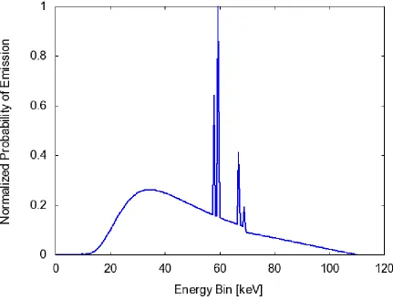
Figure 4.4 The probability density function for the spectral emission of the tungsten X-ray source used in the microCT system. . . 24

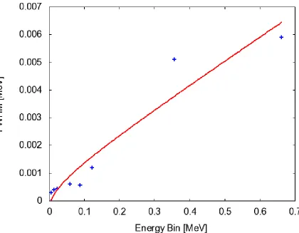
Figure 4.5 A plot of the centroids and corresponding FWHM found from the AMPTEK supplied spectra used to build the DRF. . . 32

Figure 4.6 An average response of a collected spectrum from a simulation that included a DRF and was run in an analog fashion. . . 34

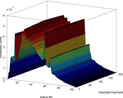
Figure 4.7 A complete spectral representation of a blank scan at a single pro-jection angle. . . 35

Figure 4.8 Demonstrating a cylinder placed in the center of the scan-able area and its respective counterpart in the form of a sinogram. . . 38

Figure 4.9 Demonstrating a cylinder placed in the center of the scan-able area and its respective counterpart in the form of a sinogram that also includes bone and various concentrations of gold within smaller cylinders. . . 39

Figure 4.10 Demonstrating a cylinder placed in the center of the scan-able area and its respective counterpart in the form of a sinogram that also includes bone and various concentrations of gold within smaller cylinders at energy bins of 20, 40, 80, and 100, which correspond to values of 22, 44, 88, and 110 keV. . . 42

Figure 4.11 Reconstructions using the MOSC algorithm with bone and various concentrations of gold within smaller cylinders at energy bins of 20, 40, 80, and 100, which correspond to values of 22, 44, 88, and 110 keV. . . 45

Figure 4.12 The original unfiltered image and three corresponding filtered im-ages with all having a kernel size of 21 and varied standard devia-tions of 1, 2, and 7 pixel spatial units respectively. . . 50

(11)

Figure 4.14 Reduced energy range of the spectral attenuation profiles from

cor-tical bone, gold, and water. . . 59

Figure 4.15 Spectral fit using the first library combination. . . 62

Figure 4.16 Spectral fit using the second library combination. . . 64

Figure 4.17 Spectral fit using the third library combination. . . 66

Figure 4.18 Spectral fit using the fourth library combination. . . 68

Figure 4.19 Spectral fit using the fifth library combination. . . 70

Figure 4.20 Spectral fit using the sixth library combination. . . 72

Figure 4.21 Spectral fit using the seventh library combination. . . 74

Figure 4.22 A cartoon representation of the object scanned where feature 100 is the sample base and the smaller sample cylinders are listed as features 1 through 6. . . 82

Figure 4.23 Successful scaling values for the bone combination fit to each voxel. 85 Figure 4.24 Successful scaling values for the water combination fit to each voxel. 86 Figure 4.25 Successful scaling values for the bone library in the bone + water combination fit to each voxel. . . 87

Figure 4.26 Successful scaling values for the water library in the bone + water combination fit to each voxel. . . 88

Figure 4.27 Successful scaling values for the gold library in the water + gold combination fit to each voxel. . . 90

Figure 4.28 Successful scaling values for the water library in the water + gold combination fit to each voxel. . . 91

Figure 4.29 Primary vote cast for the combination with the reducedχ2 redclosest to 1. . . 93

Figure 4.30 Primary vote cast for the combination with the total area under the curve closest to 100%. . . 94

Figure 4.31 Primary vote cast for the combination with the lowest maximum standard deviation between the fit and the unknown. . . 95

Figure 4.32 Primary vote cast for the combination with the lowest total stan-dard deviation between the fit and the unknown. . . 96

Figure 4.33 Final choice made for each voxel on the most appropriate library combination. . . 97

Figure 4.34 Relative intensity map of bone found with the object after Gaussian filtering of the reconstructed image. . . 99

Figure 4.35 Relative intensity map of gold found with the object after Gaussian filtering of the reconstructed image. . . 100

(12)

Figure 4.37 Relative intensity map of all three materials present within the object after Gaussian filtering of the reconstructed image where each color represents a separate material as bone is green, red is gold, and blue is water. . . 102 Figure 4.38 Nonfiltered and non-normalized material libraries used for material

quantification used with the bone, gold, and water example. . . . 106 Figure 4.39 Intensity map of bone found with the object under investigation. 107 Figure 4.40 Intensity map of gold found with the object under investigation. . 108 Figure 4.41 Intensity map of water found with the object under investigation. 109 Figure 4.42 Points used and the equation found to relate the scaling values to

the material density for bone. . . 113 Figure 4.43 Points used and the equation found to relate the scaling values to

the material density for gold. . . 114 Figure 4.44 Points used and the equation found to relate the scaling values to

the material density for water. . . 115 Figure 4.45 Density map of bone within the object under investigation. . . 117 Figure 4.46 Density map of gold within the object under investigation. . . 118 Figure 4.47 Density map of water within the object under investigation. . . . 119 Figure 4.48 A single representative density map for the materials of bone in

green, gold in red, and water in blue. . . 120 Figure 5.1 Comparison of the true density and the regional average density

found for the gold material. . . 123 Figure 5.2 Density map of bone within the object under investigation. . . 126 Figure 5.3 Density map of water within the object under investigation. . . . 128 Figure 5.4 A single representative density map for the materials of bone in

green and water in blue. . . 129 Figure 5.5 Comparison of the true density and the regional average density

found for the bone material. . . 130 Figure 5.6 Comparison of the true density and the regional average density

found for the water material. . . 132 Figure 5.7 Percent of standard deviations for the found solution densities of

bone. . . 133 Figure 5.8 Percent of standard deviations for the found solution densities of

water. . . 134 Figure 5.9 Regional averages of the percent of standard deviations to the found

densities and the corresponding local standard deviations within each region for bone. . . 135 Figure 5.10 Regional averages of the percent of standard deviations to the found

(13)

Figure 5.11 Points used and the equation found to relate the scaling values to the material density for gadolinium. . . 140 Figure 5.12 Nonfiltered and non-normalized material libraries used for the

ma-terial quantification of bone, gadolinium, and water. . . 142 Figure 5.13 Density map of bone within the object under investigation. . . 143 Figure 5.14 Density map of gadolinium within the object under investigation. 144 Figure 5.15 Density map of water within the object under investigation. . . . 145 Figure 5.16 A single representative density map for the materials of gadolinium

in red, bone in green, and water in blue. . . 146 Figure 5.17 Comparison of the true density and the regional average density

found for the gadolinium material. . . 147 Figure 5.18 Points used and the equation found to relate the scaling values to

the material density for iodine. . . 152 Figure 5.19 Nonfiltered and non-normalized material libraries used for the

ma-terial quantification of bone, gold, water, gadolinium, and iodine. 153 Figure 5.20 Density map of bone within the object under investigation. . . 154 Figure 5.21 Density map of gold within the object under investigation. . . 155 Figure 5.22 Density map of water within the object under investigation. . . . 157 Figure 5.23 Density map of gadolinium within the object under investigation. 158 Figure 5.24 Density map of iodine within the object under investigation. . . . 159 Figure 5.25 A single representative density map for the materials of iodine in

purple, gold in blue, gadolinium in green, bone in yellow, and water in red. . . 160 Figure 5.26 A single representative map of the locations for each material in

the library. . . 165 Figure 5.27 A single representative map of the locations for each material in

the library with a higher frequency 2D Gaussian filter. . . 168 Figure 5.28 The normalized and filtered libraries used from reconstructed

im-ages with five channels. . . 172 Figure 5.29 Material locations using five energy bins. . . 173 Figure 5.30 The normalized and filtered libraries used from reconstructed

im-ages with fourteen channels. . . 174 Figure 5.31 Material locations using fourteen energy bins. . . 175 Figure 5.32 The normalized and filtered libraries used from reconstructed

(14)

Chapter 1 Introduction

X-ray Computed Tomography (CT) utilizes combinations of many individual 2D projec-tions taken at different angles to produce a 3D cross-sectional image. The X-ray tubes used in these types of applications emit photons over a range of energies, which are fo-cused on the object under investigation. Traditionally, CT systems have been employed using integrating detectors to measure each of the 2D projections of the object under in-vestigation where the incident X-ray spectrum was reduced to a single value. This idea as a whole was originally conceived and introduced by Godfrey Hounsfield in 1971, and sub-sequently published in 1973. In 1975, Hounsfield built the first whole-body scanner, and in 1979 he shared the Nobel Prize in Medicine with Allen MacLeod Cormack. Since its initial implementation on the human body, modern society has deemed CT as one of the most valuable modalities for in vivo imaging due to its high-resolution, cost effectiveness, and speed of acquisition.

(15)

amount of each material. This specialized process is able to differentiate mixtures of ma-terials using a specially designed photon detector array with the capability to group the collected photons into at most 100 non-overlapping energy bins. While such a detection system is beyond the reach of current technologies, technical developments are heading in a direction to create detector arrays that are capable of resolving more and more energy bins. With this specialized detector arrangement, the full spectral photon emission from the tungsten X-ray source can be collected and used throughout the analysis process. The physical size of the detection elements is also an interesting characteristic because the reconstructed CT image has pixel sizes in the micrometer scale. This feature of the photon detector array is the defining aspect to the system used here being labeled as a microCT system.

Identifying the materials present within a CT image can become exceptionally bene-ficial to a medical team when treating a patient. In many cases, there are several medical practitioners involved in the prognosis of the patient, and these professionals can have different levels of experience as well as specific fields of study. These differences in perspec-tive can cause discrepancies in the various interpretations of the image. Considering that X-rays in general are primarily used for imaging objects with high density that contain high Z elements, for a medical practitioner to image soft tissues with low density, they may choose to introduce a metallic contrast agent into the subject. These contrast agents help reduce potential sources of ambiguity within the image, and the medical team may utilize various types of contrast agents to highlight specific regions under investigation.

(16)

(17)

Chapter 2 Background

(18)

system on a single gantry (Roessl, 2007).

(19)

2.1 CT Systems and Material Identification

One significant contribution to the X-ray CT systems development in identifying mate-rials was the use of energy-resolving photon-counting detectors in place of the preexist-ing integratpreexist-ing detectors. These improved detectors have the capability to select energy thresholds on the deposited energy of the incident photons and place counts in their re-spective energy bin or channel. Given the idiosyncratic case where the detector resolves incident photons into two separate energy groups, the system could mimic a dual-energy imaging system but in this case, there is no overlap of energy regions, wherein the tradi-tion dual-energy allows for spectral overlap. Several of these specialized detectradi-tion systems have been proposed and are still in the preliminary stages of operation (Firsching, 2004; Le, 2011; Roessl, 2007), all of which are limited by the number of energy bins, and the physical space between each detection element. Despite these conflicts, research and development in this field continues due to the approximate 30% increase in geometric efficiency of photon counting detectors over integrating detectors (McCollough, 2015).

(20)

spec-trum and the subsequent detector response (Modgil, 2015). Another approach attempts to produce separate images within the Compton and photoelectric regions for each ma-terial using multi-energy detectors. This technique explored a single emission source as well as switched-source spectral emissions to achieve its material identification and den-sity estimation. A weighted quadratic approximation to the Poisson likelihood function was used to deemphasize energy bins with low signal. The weighted sinograms were then used to perform the material decomposition on each material’s Compton and photoelec-tric profiles (Yuan, 2016).

The CT system’s ability to resolve more energy bins leads to improved spectral data, and therefore leads to an increased capability in material discrimination. These measure-ments provide discrete information about the transmitted spectra as well as spectra that has interacted with the scanned object. With a more complete spectral description of the materials, k-edge imaging is one technique that can be used to locate and detect specific materials or even multiple contrast agents (Roessi, 2011). This approach is significant in that images produced by photons have the capability to provide good image quality for objects consisting of relatively high atomic numbered elements, such as calcium in cortical bone, but possess poor contrast with low atomic numbered elements, such as hydrogen in soft tissues.

(21)

per voxel in the reconstructed image. The means by why which these nanoparticles are attached to the biological tissues is based on their ease of bioconjugation and biomodifica-tion to the targeting ligands. In addibiomodifica-tion, the metal particles have a strong drive to bond with thiol, disulfide and various amine groups that allow surface conjugation with several peptides, proteins, antibodies and other biomolecules through basic chemical processes (Sperling, 2010).

Determining materials within a CT image can lead to the identification of: the mass density, effective atomic number, or other material specific information. Currently, clin-ical applications use this information into two broad categories. The first is focused on quantifying the concentration of a certain component of a mixture, which may consist of a contrast agent, and soft tissue or fat (Kappler, 2010). The second category is a classifica-tion of the materials into predefined groups by comparing the effective atomic number or by using density independent measurements, such as the CT number at various energies (Goodsitt, 2011).

(22)

next decade until 1994 when the first worldwide commercially available microCT scanner by SCANCO Medical was introduced. This technology was initially used as a bone scan-ner and has since become a standard in bone research on the progression of osteoporosis (Ruegsegger, 1994).

(23)

2.2 K-Edges

As previously mentioned, one significant attenuation feature used in CT analysis of var-ious materials is the k-edge. To begin to understand the origins of this effect, it is first essential to understand that the electrons orbiting the nucleus of an element are orga-nized into so-called orbital levels or shells. The ”k” shell is closest to the nucleus, with ”l”, ”m”, and so on, as the shell level increases. The electrons that reside in each shell are restricted to specific quantum states within each shell and are energetically more favorable to be bound to an atom rather than freely roaming the universe (Prince, 2013). The electrons binding energy is specific to each element and shell within which the given electron resides. Given that a photon interacts with an element and undergoes a pho-toelectric absorption event and that photon has an incident energy slightly above the binding energy of the k-shell electron for that particular element, a sudden increase in the photonic attenuation coefficient is experienced (Tsoulfanids, 2011). If that photon was below the binding energy of the k-shell electron, then it would be less likely to be absorbed. As a result of this increase in the photonic absorption, an edge is created in the attenuation profile for each element at its specific k-shell’s electron binding energy and is termed the k-edge.

(24)

Figure 2.1: Photonic mass attenuation profiles of various contrast agents where the k-edges are marked and above 30 keV.

(25)

2.3 Introduction to the ACLLS Method

This body of work demonstrates a new technique for analyzing all of the materials present within a reconstructed microCT image and the capability to quantify each of the ma-terial’s concentration present. Although more emphasis will be placed on the contrast agents, quantification of all materials present within each voxel is especially important for a complete picture of the object under investigation. After locating each material within the object, this technique is then able to ascertain the density of each material within each voxel. This approach utilizes a single potential voltage X-ray tube that emits a polychromatic spectrum in the same fashion as a traditional CT image. One central aspect that is considered with this novel analysis perspective, focuses on the energy re-solving detector array used. Due to the fact that the current designs and technology to build such detectors do not currently exist today, only simulations were explored despite that similar detection systems have been constructed, but they were not built to the specifications desired.

(26)

(27)

Chapter 3 Overview of the Approach

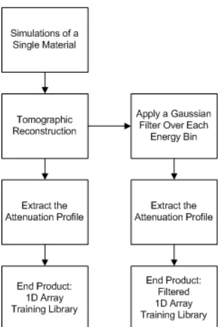
The approach used within this investigation for material identification and quantification requires a complex process. To hopefully clarify the direction taken through this journey, it was decided that an overview would be presented before unveiling each element of the complete analysis. The entire overall method can be broken down into three practical steps: 1) Simulations of single materials to build the training library, 2) Simulations of a test case with multiple materials at several densities, and 3) Testing the ALLS method to identify and quantify all materials present. Each of these three phases have elements that are similar but individualistic to each case. To best understand these phases, flow charts were made for each.

(28)

Figure 3.1: Simulations of single materials to build the training libraries.

Figure 3.1. Each material has two separate libraries that are created after simulation and tomographic reconstruction. One library is created after the reconstructed figure has been passed through a 2D Gaussian filter over each energy bin, which serves as the library for identification of the materials present. A second library is generated directly from the tomographic reconstruction and used to quantify the amount of materials present after identification.

(29)

Figure 3.2: Simulations of a test case with multiple materials at several densities.

locations to the ACLLS. Throughout this investigation, variations on the materials and concentrations were studied and were all created in this same manner.

(30)

(31)

(32)

Chapter 4 Methods

(33)

inherent non-linearity, resolution, and efficiency. All of the of these semi-empirically de-rived characteristics were grouped together in the detector response function (DRF) that was applied directly within the MCNP6 simulations. An initial analysis using the ACLLS analysis package utilized a 2D Gaussian filtered image that was then normalized to begin the material identification process. In order to further enhance the appropriate material library selection for the ACLLS analysis, predetermined threshold criteria on the validity of the fit from the library combinations were used to ignore unlikely candidates. These specific values were determined empirically, and of the remaining material combinations, votes were cast on additional statistical criteria to govern the final identification of the materials in each voxel. After this identification process, a second linear fit was made using the selected material library combination for each voxel to the original image that was unfiltered. This fit was then used to make an assessment of the physical amount of each material present within the voxels.

(34)

4.1 Micro CT System Design

An essential aspect of any CT imaging device is to completely understand the imple-mentation of each individual hardware component so as to produce the most accurate reconstructed image feasible. Considering that the focus here is placed on microCT sys-tems, the instruments used will all be quite small. The basic geometry of the physical device mimics previous work by Gonzales in 2011, which was originally designed as a dual spectrum microCT system where he modified the device to account for changes in the detector apparatus used. Here, the detector was again changed and as a result, only simulations were possible as a means to continue exploration of material identification and quantification.

(35)

lead. The reason for the single layer of detection elements resides in the desire to explore the feasibility of material identification and quantification rather than to generate three spatially dimensional figures. As a result of this one dimensional detector array, the height of the sample used is somewhat arbitrary, but so as to produce a constant reconstructed image and for the sake of clarity, the height of the sample was limited to 4.0 cm. Several visual representations of the microCT system used that can be seen in the following figures.

Figure 4.1: A to-scale side view of the microCT system used.

Figure 4.2: A to-scale top view of the microCT system used.

(36)

Figure 4.3: A to-scale isometric view of the microCT system used.

each figure. It should also be noted that each of these figures are to scale in each view. A spectral emission of a 110 kVp tungsten X-ray tube was used as the source of pho-tons. It was modeled as a point source that has been collimated into a cone of directions centered on the detector array. The half-angle of the cone has been constrained at 3.18 degrees, which is slightly larger than the detector array itself. Each angle has been equally weighted which will ensure an even distribution of photons and that all straight line pro-jections are possible throughout the simulation. It is important to keep in mind that the original Gonzales work implemented a pencil beam photon emission, which creates a substantially different spectral response. The driving factor behind these differences are that the scanning pencil beam and single-pixel detector arrangement would result in substantially more scatter rejection but also require considerably more scanning time. The photon emission profile in this discussion used a cone-beam system which will have a different impact on the collected scattered photons.

(37)

of the X-ray device, and the cut-off at the highest energy of 110 keV which is defined by the applied voltage to the anode of the X-ray device. Between the roll-off and the cut-off extremes lies a triangular shape which is defined by the Bremsstrahlung radiation gen-erated by electrons within the X-ray tube. The remaining features are the characteristic peaks which are the result of the fluorescence radiation based on the target of the X-ray device used, tungsten in this case. This emission spectrum was the only X-ray source used during this investigation but further optimizations could be explored in the future.

(38)

The detector array chosen for this application that consists of 200 individual elements, and has been chosen specifically with the future in mind. As it currently stands within the industry, the number of divisions that the incident spectra on the detector array can be split into is relatively low, at less than 10 energy bins (Anderson, 2010). Here, it was assumed that the technology to separate the spectra into a larger number of energy bins will continue to improve. An example of this advancement can be seen in that a single photon-counting detector element has been constructed by AMPTEK, which can differentiate up to 1024 energy bins between 10 and 100 keV. In 2011, Gonzales was able to demonstrate that a microCT image could be generated by taking multiple measurements using this single AMPTEK detector at varying positions along an axial direction. This approach mimics a one dimensional strip detector array and was used at various projection angles to produce the final reconstructed cross-sectional image. One large setback from using this approach for practical in vivo use, is that it requires a very long scan time to achieve reasonable spectroscopic reconstructions.

(39)

(40)

4.2 Simulation of the Model and the Detector

Re-sponse Function (DRF)

It should be noted that the detector array designed in this application specifically for a microCT system with the capabilities to resolve a large number of energy bins does not yet exist. As a result of the detector array’s hypothetical nature, the only means by which this investigation could continue was through the use of radiation transport simulations. Monte-Carlo simulations offer the most robust parameters in regard to changes in geome-try and material properties, and were deemed as the most appropriate means to generate realistic raw microCT data. The transport code chosen which is export controlled and reg-ulated by the Radiation Safety Information Computational Center (RSICC) was Monte-Carlo N-Particle (MCNP v. 6.1). This particular transport code system was chosen as the simulation package due to its general-purpose, continuous-energy, generalized-geometry, and time-dependent capabilities. Other Monte-Carlo radiation transport packages exist such as Geant4, Penelope, and FLUKA but the authors chose to use MCNP out of fa-miliarity. All of these software packages should produce statistically similar results and could have been subsisted for MCNP.

Another point to consider, with respect to the detector’s design, resides in the compu-tational time required to complete each simulation. As the number of spectral divisions increases, so does the amount of computation time required to produce a statistically viable solution. The use of an in house computer cluster of many CPU’s allowed for an acceleration in the completion of this task. This was another facet used in selecting MCNP as the simulation package to complete the necessary projections.

(41)

would most accurately represent reality. These decisions were centered on the various physics models that MCNP would implement. A complete physics package was cho-sen where detailed photon physics were treated over the range of emitted X-rays. This included the generation of bremsstrahlung photons, coherent scattering or Thompson scattering, incoherent scattering or Compton scattering, and Doppler energy broaden-ing. Also, analog capture was used over Russian roulette to ensure proper sampling of all interactions with each material.

The F8 deposited photon energy tally was used on each of the individual 200 CdTe detector elements that constituted the entire detector array. The deposited energy sim-ulated in MCNP was then placed into one of 100 energy bins that were equally and linearly spaced between 0.0 and 110 keV. These energy depositions were then used to estimate the energy distribution of light pulses created from scintillation events within the detector’s materials. In reality, each of these light pulses are then converted into an electrical pulse through the use of the photomultiplier tube or PMT. Through the process of the scintillation event and the eventual production of a measurable electrical pulse, the relationship of the energy of the incident photon to that of the scored event is known as the detector response function (DRF).

(42)

characteristic width is dictated by the specifics of the detector used.

G(x) = 1

σ√2πe

−(x−µ)2

2σ2 (4.1)

Equation. 4.1 is the probability density of the Gaussian distribution where: x is the observed data point,µ is the average value, andσ is the standard deviation. Within the MCNP simulation package the peak can be broadened using a Gaussian Energy Broad-ening (GEB) function where the incident photon is dealt with by changing the energy of the particle during the simulation just before it is tallied by randomly sampling based off of predefined Gaussian distribution. This probability distribution function (PDF) is supplied by the user where the desired Full Width at Half Maximum (FWHM) of the Gaussian distribution is defined by Equation. 4.2.

F W HM =a+b+√E+cE2 _(4.2)

Within Equation. 4.2, E is the energy of the photon in MeV, and a, b, and c are constants provided by the user. It should also be noted that the Gaussian standard deviation and the FWHM are related and can be derived and approximated to take the form found in Equation. 4.3.

F W HM = 2.35σ (4.3)

(43)

photon peak placed along the x-axis at its incident energy and then it is paired with its corresponding FWHM along the y-axis to demonstrate their relationship. Ideally, these photon peaks would not be convolved with other collected photons and would be isolated. This can become cumbersome when using an X-ray tube due to the intrinsic Bremsstrahlung emission profile that will cause the Gaussian fitting of the full energy peaks to be slightly off. Ideally, radioisotopes that emit a mono-energetic photon would be used. Separate radioisotopes would be chosen to represent a wide range of energies so as to construct a complete profile of the DRF. Choosing the specific radioisotopes can also cause problems, especially when attempting to characterize low energy photons. Lower energy photons are typically accompanied with higher energy gamma-rays that were emitted from the radioisotope at hand. Due to photonic interactions of the higher energy gamma-rays, their Compton continuum can impact the lower energy photon’s centroid and FWHM. The result of these various constraints on the accuracy of both the photon’s centroid and its corresponding FWHM causes the definition of the DRF to require very close attention to detail about the spectra used.

Given that the chosen detector array employed in this application was based off an existing AMPTEK design, information data sheets that are publicly available by AMPTEK were used to construct the needed DRF. By not having direct control over the radioisotopes used in the provided AMPTEK information, less than ideal radioisotopes were chosen. Also, by not being able to choose the applied voltage to the detector, the number of energy bins collected over, and the gain on the signal produced, complete and consistent spectral responses cannot be guaranteed for the purposes of creating the DRF. Regardless of these limitations, the radioisotopes, centroids, and FWHMs used to create the DRF can be found in Table 4.1.

(44)

Table 4.1: The radioisotopes, centroids, and FWHMs used to create the DRF.

Element Centroid [MeV] FWHM [MeV] Fe55 0.00590 0.00029 Am241 0.01395 0.00039 Cd109 0.02210 0.00043 Am241 0.05954 0.00060 Cd109 0.08800 0.00057 Co57 0.12200 0.00120 Ba133 0.35600 0.00510 Cs137 0.66200 0.00590

Equation. 4.2 was used as the fitting parameters to be applied within MCNP to assist the simulations in producing an accurate representation of the spectra. The found values for a , b, and c are: -0.00035001, 0.0046523, and 3.3393 respectively. A scatter plot of the points used as well as a continuous plot of the fit to create the DRF can be found in Figure 4.5. Ultimately, the values used in the DRF are not ideal, but considering that the entire detector array has not been developed, the specifics are somewhat irrelevant. The supplied data and subsequent DRF will adequately represent the hypothetical detector array for this application.

(45)

(46)

a means to accelerate a solution, a computer cluster of 160 CPUs were employed. Enough histories were executed so that each energy bin of every detector had an associated relative error of at least 5%, which is recommended by the MCNP manual.

An average response of the collected spectrum that has met all of the desired simula-tion characteristics can be found in Figure 4.6. Also, no objects were placed between the source and the detector array within the simulation. Within Figure 4.6 the characteristic X-rays from the tungsten photon source can be easily identified at approximately 59 and 69 keV. The peaks that arise below the 40 keV energy bin are characteristic peaks that arise from the CdTe detector itself and the surrounding lead. The actual values of the spectrum are the number of counts that have been normalized to the number of histories sampled. These values would then be multiplied by the number of photons emitted by the X-ray device to represent the ideal measurement. At this point, Gaussian or Pois-son distributed noise can be added to even better represent an experimentally collected spectra.

(47)

(48)

(49)

The information to complete a tomographic picture requires measurements to be taken at many different angles. Although not always essential, but for this discussion it was deemed that a complete 360-degree scan would be easier to process and reconstruct, as well as reduce the amount of reconstruction artifacts. It is possible to produce a reconstruction from a ”short scan” which is less than a complete 360-degree scan but these reconstructions do not provide redundant angles and results in less information. Given that a full 360-degree scan was chosen, the angular sampling size, which dictates the number of projections taken, was set to be acquired every two degrees. Unfortunately, this sample size does not fulfill the basic rule of thumb given the size of the detector array and that the number of sample angles be greater than 1.5 times the number of detection array elements. The outcome of this sample size results in some tomographic artifacts despite the fact that the object’s projection does not reach all 200 detection elements. The total number of angular sampling dictates a total of 180 individual projections where each needs a separate MCNP simulation to represent the rotational change in geometry. To further ensure that the simulations generated from each projection angle would be individual, the seed used to spawn the random number generator critical to any Monte-Carlo simulation was chosen to be different for each MCNP run. The total number of data points for a single microCT scan used in this discussion is based off of 200 detector elements with each having 100 energy bins collected at 180 separate projection angles. This sums to be a total of 3.6×106 _{data points that needs careful organization before it}

(50)

4.3 Image Reconstruction

The first step in translating the large amount of data into something that is a better cross-sectional representation of the object at hand is to turn the data into a sinogram. A sinogram is not to be confused with a sonogram, which is created from an ultrasound echo response and most notably associated with measuring and imaging fetuses. Sino-grams are a specific form of visual representation that the raw data collected from a tomographic scan is turned into before reconstruction can begin. The reason that the visualization is called a sinogram stems from the fact that during the data collection phase, photons pass through a fixed central point in the object based on the projection angle that corresponds to a location on the unit circle. To the unfamiliar, a sinogram can be confusing to interpret. The x-axis usually represents the detector array were the center of the array is the center of rotation and correspondingly, the y-axis in a sinogram typically represents the projection angle that was used to collect the data.

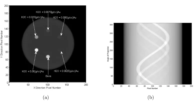
A very basic example of a sinogram can be found in the following figures where the straightforward sample base without any smaller cylinders placed inside was investigated. Figure 4.8a and Figure 4.8b are demonstrating the single cylinder filled with a single material (water in this case) on a blank background. Figure 4.8a is a reconstructed image of the object, and Figure 4.8b is its corresponding sinogram. The sinogram reveals that the object’s center is exactly in the middle of the center of rotation by there being no drastic variation about the pixels. It is also apparent that the edges of the cylinder in the sinogram are fading away due to the lack of physical material attenuating the emitted photons.

(51)

(a) (b)

Figure 4.8: Demonstrating a cylinder placed in the center of the scan-able area and its respective counterpart in the form of a sinogram.

corresponding sinogram in Figure 4.9b where these images better represent the complete model being used throughout this discussion. Within Figure 4.9a, the same water base as in Figure 4.8a can be seen, but in this instance at a lesser relative intensity value. The reason for this drop in relative intensity can be found with the inclusion of a single cylinder being filled with cortical bone and the remaining cylinders being filled with various concentrations of gold contrast mixed with water. Since these cylinders have a higher density, they appear brighter which is a result of the plotting software normalizing to the highest value within the image. This geometric arrangement will serve as the primary example throughout this discussion.

Figure 4.9b demonstrates the corresponding sinogram where there are clear repre-sentations of a sine wave like shape as the angles progress from the 0th _{degree to a full}

rotation at the 360th _{degree. Each of the sine waves represent a separate cylinder filled}

(52)

the relative density of the object scanned. Facets of the sinogram representation of the object can become exceptionally complicated when multiple objects overlap causing an additive effect in the image. The consequences of the summations of denser cylinders can be most easily seen along the 65th _{pixel of Figure 4.9b. Another aspect of the sinogram}

is that some of the features are difficult to visually represent such as the cylinders with lower gold concentration.

(a) (b)

Figure 4.9: Demonstrating a cylinder placed in the center of the scan-able area and its respective counterpart in the form of a sinogram that also includes bone and various concentrations of gold within smaller cylinders.

(53)

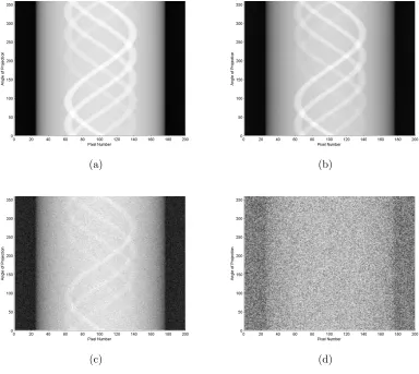
that energy spectra are produced from every detection element and therefore a resulting sinogram can be generated from each energy bin as demonstrated in Figure 4.7. If every available energy bin was used to reconstruct a tomographic image, then the complete data set would comprise one hundred separate sinograms. One possible means by which to show this comprehensive information is through a motion picture like representation, where every energy bin sinogram would progress one after another. Unfortunately, it is impossible to demonstrate a motion picture in a written form, so several energy bin rep-resentations are shown in Figure 4.10a through Figure 4.10d. Within this series of images, the same geometric and physical construction was repeated as from figure Figure 4.9a, but in this instance the energy discriminating detector array was used.

Considering that the photon emission spectrum from the source varies with energy, so will the response of the materials within the object scanned and their result will be captured by the detectors. These photonic variations about the energy can be seen in the four separate images of Figure 4.10a, Figure 4.10b, Figure 4.10c, and Figure 4.10d, where the energy bins represented are 20, 40, 80, and 100 with their respective energies as 22, 44, 88, and 110 keV. The relative intensities obviously are different between each of the energy bin sinograms, where in the 20th _{energy bin, there is relatively low noise and the smaller}

gold objects are closer in intensity to the surrounding water. Within the 40th _{energy bin}

sinogram, the gold objects stand out much more distinctly than the water. As the energy bins progress to higher values as in the 80th_{energy bin, photonic noise plays a much larger}

(54)

by the PDF. Lower energy bins may experience higher than anticipated counts due to the materials that the photons interact with, which can be accounted for from single or multiple down-scattering events.

Now that all of the MCNP simulated spectra have been transformed into sinograms at all of the available energies, the actual reconstruction of the data into a CT image may occur. The process of reconstructing any CT image can be computationally intensive and may cause errors to arise. Traditionally, the Feldkamp or FDK algorithm has been used for reconstructing 3D X-ray CT systems with a cone beam emission (Feldkamp, 1984). One particular area where the FDK algorithm begins to perform poorly is when there are truncated ill-conditioned geometries with respect to the photon projections or when there is sparsely collected data. Whereas the FDK algorithm is an analytical solution to the reconstruction process, iterative algorithms have been shown to have the capabilities to solve non-traditional geometries and poorly sampled projections with improved image quality over analytical solutions. The largest draw back from using iterative solutions to produce a CT reconstruction is that they require a large amount of computational power. Due to this constraint, much effort has been placed on finding a fast and efficient iterative algorithm to produce a reconstructed image within a timely manner.

(55)

(a) (b)

(c) (d)

(56)

in choosing the MOSC algorithm was that during its testing of a limited-angle microCT system, the results demonstrated that there was little image degradation to the spatial resolution and a nominal impact on the noise level in the image when compared with the OSC reconstructed image. Additionally, the MOSC algorithm estimates the linear attenuation coefficients within each separate voxel of the reconstruction, which further assists in producing an accurate reconstruction of the object under investigation.

The 10th iteration of the MOSC reconstruction process was deemed as the most ap-propriate solution to use as a means to determine the material properties of the scanned object. The tenth iteration was chosen because a property of the MOSC algorithm’s reconstructions is that as the number of iterations becomes too large, high frequency fea-tures within the object become more pronounced. There is essentially a trade-off between maintaining high-frequency features while trying to reduce the unwanted noise within the reconstructed image.

The MOSC reconstruction process does not use information based on the energy bins above and below the bin that is being reconstructed, and as a result, each of the previously constructed sinograms act independently. The only caveat in regards to the separate energy bins is that each energy bin requires a separate blank scan which will vary at every energy bin. These separate changes are visually represented in Figure 4.7. In the future, there may be an inclusion of a reconstruction technique that would be able to utilize information collected by the same detection element at energy bins below and above the one at hand to improve the overall reconstructed image quality. This idea was proposed in the work by Gonzales, where post-reconstruction smoothing on the spectral aspects were performed using an eigenvector decomposition approach, but this idea was not implemented here (Gonzales, 2011).

(57)

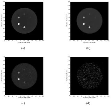
and Figure 4.10d, Figure 4.11a,Figure 4.11b, Figure 4.11c, and Figure 4.11d demonstrates each of their MOSC reconstructions. Again, the entire reconstructed image is represented by a full 100 energy bin range, but a small sample set of the energy bins displayed in the corresponding figures are 20, 40, 80, and 100 with their respective energies as 22, 44, 88, and 110 keV. Within the 20th _{energy bin shown in Figure 4.11a, there are some}

image artifacts between the lowest cylinder, which is bone at the approximate location (100,70) the cylinder located at the lower left corner, which has the highest concentration of gold at the approximate location (70,80), and the cylinder at the top left, which has the next highest gold concentration at the approximate location (70,120). These three cylinders are the most dense features in the object under investigation and as a result, a beam-hardening like artifact can be seen forming a triangle between the three cylinders. The means by which a microCT image is acquired and able to differentiate various features is centered on the fact that different materials attenuate and scatter the X-rays passing through them. Given that a suitable energy of incident photons is used so that the attenuation is dictated by the photoelectric effect while also allowing for scattering of the photons out of the detectable field of view, the relative intensity of the transmitted X-rays can be found to follow the incident X-rays by the definition in Equation. 4.4.

I =I0e

−(µ_ρ)ρx

(4.4) Within Equation. 4.4,I0is the incident intensity of photons on the object andI is the

(58)

(a) (b)

(c) (d)

(59)

(60)

4.4 Preprocessing the Reconstructed Image with a

Gaussian Filter

After the simulations were completed and the MOSC reconstructions had produced an image for each energy bin, it was found that passing each energy bin image through a 2D spatial filter improved the material selection process. A Gaussian smoothing filter was used and was implemented as a convolution operator where its primary function was to remove high frequency noise through a blurring like action. Ultimately, the Gaussian filter acts as a rotationally symmetric lowpass filter, where the operator is simply the product of two 1D Gaussian functions as in Equation. 4.1 where both the x and y directions are represented. The actual implementation of the Gaussian smoothing lowpass filter on the reconstructed image can be found using Equation. 4.5 and Equation. 4.6.

hG(x, y) =

1

σ√2πe

−x2+y2

2σ2 _(4.5)

h(x, y) = _P hG(x, y)

x

P

yhG(x, y)

(61)

only contain values within three standard deviations, that hardly any information will be unaccounted for throughout the filtering process.

To ensure a consistent result, the same square kernel size and standard deviation of the Gaussian distribution was used on each reconstructed image produced from every energy bin. The foundation for this thought process was to generate an evenly distributed filter in both the x and y directions and intensities regardless of the object under investigation. The standard deviation value needs to be low enough to ensure that the image will not result in a completely flat figure, with some of the high frequency edges remaining while removing a large portion of the noise. The size of the kernel was chosen as an odd number to place the most emphasis on the center most voxel, and it must be substantially large enough to account for more than just three standard deviations of data points.

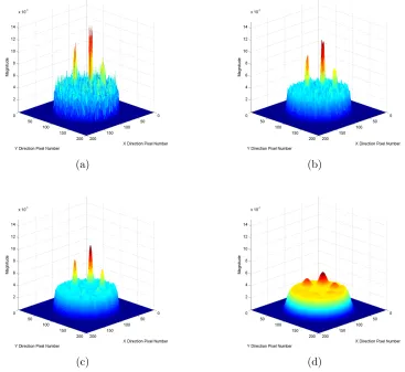
To demonstrate the process on how the specific values of the base kernel size and the standard deviations were chosen, a range of parameters were explored. For this demon-stration, the same geometric construction, material properties, and energy bin were used as in Figure 4.11c. Within this specific data set, there is a large amount of noise at the 88 keV energy bin reconstructed image. This noise is dominated by the lower number of photons emitted from the PDF of the X-ray tube with a smaller contribution from the reconstruction itself. Also, by using this energy bin’s reconstructed image, the k-edge of gold attenuation profile stands out as having a brighter signal than its surrounding mate-rials. With the intention to exhibit the various changes in the most dominating feature of the Gaussian convolution filter, the kernel size was held at a constant value of 21, while the standard deviation was varied.

(62)

These standard deviations were chosen to demonstrate the three main cases of: not enough filtering, sufficient filtering, and a filter that smoothed the image too much. Figure 4.12b demonstrates an image that has not undergone a sufficient amount of filtering because in this example, there is still a large amount of noise and the features are not as distinct as desired when compared to the original unfiltered image. Figure 4.12c displays the case that was found to be the most ideal for the ultimate goal of material identification. When a standard deviation of 2 spatial units was used, it produced a Gaussian filtered image that preserved the edges of the features desired, specifically the edges of the objects containing bone and various mixtures of gold. It also reduced the overall noise within each feature, as well as the object as a whole and maintained some resemblance of the general magnitude from the original unfiltered image. Figure 4.12d is at the upper most extreme of the acceptable range of the kernel used with a standard deviation of 7 spatial units. Here, the image has been drastically smoothed and the edges of all the features have been blurred together. While this amount of filtering has the lowest amount of noise, the least amount of original information has been preserved from the original image and has a large potential to produce incorrect solutions on the materials present within any voxel.

(63)

magni-(a) (b)

(c) (d)

(64)

(65)

4.5 Building the Libraries of the Material’s

Attenu-ation Profile

After the simulations, complete reconstruction, and Gaussian 2D filtering of the desired model has finished its computationally laborious tasks, the attenuation profiles of the known materials need construction. Considering that spectral data exists for each recon-structed voxel, the tools able to utilize the increased information needed development. To accomplish this, the All Combinations of the Library Least Squares (ACLLS) analysis tool was created to make comparisons with known spectral solutions to each spectrum created within the reconstructed image’s voxels. Through utilizing spectral combinations of elements and material compounds, the correct solution was chosen but before any of this specialized analysis can be performed, the attenuation profiles for each of the libraries needed to be built.

(66)

potential candidates, a material identification can be made as well as quantification of the materials present within the voxel at hand. Combinations of the libraries are used because the order in which the materials are grouped together does not matter to the found solution, whereas permutations are order dependent

The libraries themselves are an integral part to material identification. Libraries and their constituents could also be considered as a training set or a series of basis functions. In this instance, the libraries are more specific to the individual situation at hand and utilize a large amount of preexisting knowledge of the apparatus used and their spe-cific behaviors. The libraries were constructed in the same fashion as the object under investigation, so as to limit the number of unknown parameters throughout the entire inverse analysis process. The reason behind this was to create a known scenario for a known material to make a valid argument that the material is or is not present in the unknown object. In order for these parameters to remain true, the specific attenuation profiles must be created using the exact same detectors as well as the exact same photon emission spectrum as the object undergoing material identification. With keeping these conditions unchanged, identifying features will remain consistent, such as characteristic X-rays derived from the detector array itself. Ultimately, the goal was to create a congru-ency between the known and unknown profiles created which can only be accomplished after the same image reconstruction process.

(67)

be represented in Figure 4.8b but depending on the material used to build the library, the intensity would be varied.

Since the MCNP simulated projections for each material should be statistically iden-tical, only projections from the 0th degree up to the 30th degree were actually simulated at two degree intervals. The rationale behind this was primarily based on the reduction of time required to simulate a complete 360-degree scan, which could take up to approxi-mately two weeks. To produce a complete sinogram with a limited data set, the simulated spectra was correctly placed in their corresponding angle positions up to the 30thdegree. The remaining projections from the 32nd _{degree to the 358}th _{degree were randomly filled}

with one of the lower angle projections. This process creates a more evenly distributed figure after the MOSC reconstruction due to multiple projections being used. If only a single simulation was used and repeated throughout all of the angles of projection, then noise created from the Monte-Carlo radiation transport process would manifest itself as a ringing artifact in the reconstructed image.

After the complete MOSC reconstruction, an average was taken over the center por-tion of the figure created at each energy bin and then assembled to produce a single representative attenuation profile. This was to help ensure that a more general shape of the attenuation profile would be preserved for each material and that random noise and undesired artifacts would be diminished. Another library was also taken in the exact same manner from the Gaussian filtered reconstructed image. Ultimately, each material had two libraries generated, unfiltered and filtered, the rationale behind this will be explained in a later chapter.

(68)

(69)

(70)

4.6 The All Combinations of the Library Least Squares

(ACLLS) Approach

The means by which the input unknown attenuation profile and the chosen library com-bination are solved utilizes the ACLLS analysis, which had not been developed in its form until this investigation began. The basis for this analysis approach is an extension and addition of multiple combinations of the well tested Library Least Squares (LLS) technique first developed by Verghese and Gardner in 1988. The LLS technique was cho-sen as an inverse solving package because it has proven itself to be successful for inverse elemental and material identification of prompt gamma-ray neutron activation analysis, energy-dispersive X-ray fluorescence analyzers, and the characterization of cargo con-tainer photon shielding.

The fundamental basis for the complete ACLLS (and the LLS) solving package has been dubbed CURMOD, which is based on the CURFIT subroutine developed by Beving-ton, and has served as the backbone for many specialized code developments (BevingBeving-ton, 1968). CURMOD can be used to describe a data set using any combination of linear and non-linear parameters. Accurate guesses are required for each non-linear parameter but they are not required for the linear parameters. CURMOD uses the Levenberg-Marquardt non-linear search method for finding a solution to the non-linear parameters and a mul-tiple linear regression in determination of the linear parameters. It uses a minimized reducedχ2 _{found in Equation. 4.7 to select the best fit for all of the parameter values.}

χ2_red= χ

2

ν =

1

ν

X(O−E)2

σ2 (4.7)

(71)

ob-servation,Ois the observed data andE is the theoretical data. CURMOD also quantifies the error σ associated with each parameter for the final fit to the input data set.

For this particular application, only linear parameters were used and as a result, each of the input library combinations had a final associated scaling multiplier for each com-ponent to the library. Each library multiplier was being used to fit the known library combination to the voxel’s unknown attenuation profile. The ACLLS fitting approach with all of its various possible combinations are determined by the number of libraries used throughout the analysis of the physical subject at hand. This is dictated by Equa-tion. 4.8, which calculates the number of combinations of r objects from a set of n

objects. This equation can then be used to calculate the total number of combination objects possible for a given set of objects.

f(n, r) = n!

r!(n−r)! (4.8)

f(n) =

n

X

r=1

n!

r!(n−r)! for

n >1 (4.9)

(72)

spectral profiles. Additionally, this example and all initial stages of the ACLLS uses the filtered reconstructed libraries in combination with an unknown image that has undergone Gaussian filtering.

Figure 4.14: Reduced energy range of the spectral attenuation profiles from cortical bone, gold, and water.

(73)

found later when the most correct library combination is chosen. Additionally, ACLLS calculates from the library fit to the unknown profile: the linear correlation coefficient

(74)

The test case attenuation profile is known to contain a combination of gold and water and for the remainder of this discussion, will be referred to as the input unknown. Analysis using the first combination of ACLLS used only the bone profile as the library to fit the input unknown attenuation profile. The results can be found in Table 4.2 as well as the plot of the input and found solution in Figure 4.15.

Table 4.2: Results from the first combination.

Name Multiplier %Error R %Area Bone 89.2591 0.0002 0.8987 0.9666

χ2

red = 1.4933

(75)

(76)

The second combination implemented only the gold profile as the library to be used to fit the input unknown attenuation profile. The results can be found in Table 4.3 as well as the plot of the input and found solution in Figure 4.16.

Table 4.3: Results from the second combination.

Name Multiplier %Error R %Area Au 124.4131 0.0002 0.9954 0.9698

(77)

(78)

The third combination implemented only the water profile as the library to be used to fit the input unknown attenuation profile. The results can be found in Table 4.4 as well as the plot of the input and found solution in Figure 4.17.

Table 4.4: Results from the third combination.

Name Multiplier %Error R %Area H2O 63.2200 0.0002 0.9091 0.9167

(79)

(80)

The fourth combination implemented the bone and gold profiles within the library to be used to fit the input unknown attenuation profile. The results can be found in Table 4.5 as well as the plot of the input and found solution in Figure 4.18.

Table 4.5: Results from the fourth combination.

Name Multiplier %Error R %Area Bone 44.0340 0.0014 0.8987 0.4769 Au 65.8635 0.0013 0.9954 0.5134

(81)

(82)

The fifth combination implemented the bone and water profiles within the library to be used to fit the input unknown attenuation profile. The results can be found in Table 4.6 as well as the plot of the input and found solution in Figure 4.19.

Table 4.6: Results from the fifth combination.

Name Multiplier %Error R %Area Bone 85.4836 0.0009 0.8987 0.9257 H2O 2.8270 0.0198 0.9091 0.0410

(83)

(84)

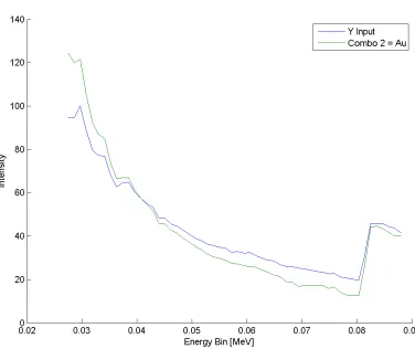
The sixth combination implemented the gold and water profiles within the library to be used to fit the input unknown attenuation profile. The results can be found in Table 4.7 as well as the plot of the input and found solution in Figure 4.20.

Table 4.7: Results from the sixth combination.

Name Multiplier %Error R %Area Au 81.5289 0.0007 0.9954 0.6355 H2O 24.9720 0.0012 0.9091 0.3621

(85)

(86)

The seventh and last combination implemented the bone, gold, and water profiles within the library to be used to fit the input unknown attenuation profile. The results can be found in Table 4.8 as well as the plot of the input and found solution in Figure 4.21.

Table 4.8: Results from the seventh combination.

Name Multiplier %Error R %Area Bone -3.5765 -0.0358 0.8987 -0.0387 Au 83.6709 0.0011 0.9954 0.6522 H2O 26.4939 0.0023 0.9091 0.3842

χ2

red = 0.1095

(87)

Figure 4.21: Spectral fit using the seventh library combination.

As it can be seen, the ACLLS analysis produces a large amount of data to process and sort through in an attempt to deduce the correct result given the situation where the correct solution is unknown. Also, keep in mind that this amount of data is produced for each individual voxel that is located within the reconstruction space.

(88)

object under investigation is taken into consideration, then several combinations can be ignored altogether. In this case, the gold contrast agent present in the sample and its specific target based on the molecule it has been bioconjugated with, can result in the removal of some library combinations. Continuing with the previous example where wa-ter, bone, and gold were used as the complete library, it could be presumed that several of the combinations were not possible. In this particular example, water was used as a substitute for tissue, and it has been assumed that gold could only bond with tissue based on its bioconjugation agent. This results in the combinations of bone + gold, and water + bone + gold impossible to determine a correct material identification because they are physically unable to be present within a single voxel. Regardless of the physical presence of library combinations, the ACLLS has the mathematical capabilities to produce a suc-cessful fit to any given attenuation profile, but the result may be meaningless and should be ignored as in Table 4.8, where the bone contribution is negative. Having knowledge of what material mixtures are physically possible has reduced the number of combinations. Also, since all of the libraries were normalized, and the input unknown was normalized and scaled, it is not realistic to have a negative scaling factor for any material, which results in any solution that is negative to be ignored for further analysis.

Once the most obvious combination solutions that are unrealistic have been ignored, user defined parameters are implemented in an attempt to reduce the combinations fur-ther. These include removing: significantly high χ2

red values, low R values, low values of

material contribution to the area, low total percent area, high total standard deviations, and a high maximum value of the standard deviation of the fit. The specific values for the thresholds were determined empirically and set at the threshold values of a combi-nation solution having a χ2

red larger than 5.0, or the total standard deviation of the fit

(89)

ignored. Additionally, a solution with any individual component solution that has an R

value less than 0.4, or a percent of contribution to the area under the curve less than 2% would be ignored. These specific values were used throughout this entire investigation and empirically chosen.

With all of the combinations removed that were deemed as unacceptable, a final selection process is able to occur. Continuing with the example from above, the only remaining combination is the correct choice for the materials present within the voxel at hand, which is the sixth combination, a mixture of water and gold. The voxel chosen for this example was located in the center of the gold and water feature with the highest concentration of gold, positioned in the lower left hand corner of Figure 4.11a through Figure 4.11b. This scenario is an ideal case where only one combination remains and proves as the only result when the number of libraries are low and there are less mixtures present within the object under investigation.