KUNG, MEIFEN. Information-based Group Squential Tests With Lagged Or Cen-sored Data. (Under the direction of Professor Anastasios A. Tsiatis.)
Conventionally, values of nuisance parameters given in a statistical design are often erroneous, thus may result in overpowering or underpowering a test using tra-ditional sample size calculations. In this thesis, we propose to use Fisher Information data monitoring in group sequential studies to not only allow an early stopping in a clinical trial but also maintain the desired power of the test for all values of nuisance parameters. Simulation studies for the simple case of comparing two response rates are used to demonstrate that a test of a single parameter of interest with a specified alternative achieves the desired power in information-based monitoring regardless of the value of the nuisance parameters, provided that this parameter of interest can be estimated efficiently. The emphasis in this part is to show how information-based monitoring can be implemented in practice and to demonstrate the accuracy of the corresponding operating characteristics in some simulation studies.
by
MEIFEN KUNG
A dissertation submitted to the Graduate Faculty of North Carolina State University
in partial fulfillment of the requirements for the Degree of
Doctor of Philosophy
STATISTICS Raleigh
2000
APPROVED BY:
Biography
Acknowledgements
I always consider myself a very fortunate person. People offered great advices and companionships at each stage of my life. I can not acknowledge them all but I am forever grateful at heart.
To my advisor Dr. Anastasios A. Tsiatis, I can not thank you enough for taking me under your supervision, leading me through my interest in applied fields, providing guidance when I needed yet giving me plenty of freedom in trying my hands. It’s a great pleasure working with you.
To my first year academic advisor Dr. Sastry Pantula, thank you for all the support and help. Without you, I might not be able to hold on at the first year.
To Dave & Kath, thank you for all the wine tastings and delicious dinners. To Volkan & Rukiye, thank you for sharing the mystery of pregnancy and the cutest baby boy Alper. His smile always warm my heart. To Ann, Noi and my long term friend Christine, your friendships are precious to me. To Chu & and Fang, thank you for sharing your home with me.
Contents
List of Tables vi
List of Figures vii
1 Introduction 1
1.1 Introduction . . . 1
1.2 Classical Sequential Methods . . . 2
1.3 Group Sequential Methods . . . 3
1.4 Outline . . . 5
2 Nuisance Parameters Free IBM 9 2.1 Introduction . . . 9
2.2 Information-based Monitoring in Group Sequential Studies . . . 12
2.3 Simulation Studies . . . 16
2.4 Summary . . . 18
3 IBM with Lagged or Censored Data 21 3.1 Introduction . . . 21
3.2 Notation . . . 23
3.3 A Consistent Estimator And Its Martingale Structure . . . 24
3.4 Sequential Joint Distribution with Censored Data . . . 27
3.5 Application in Comparing Two Response Rates . . . 29
3.6 Simulations . . . 31
3.7 Future Approach . . . 34
List of Tables
1.1 Effect of Multiple Looks at the Nominal Level . . . 8
2.1 MI values in all 3 cases of interests for both matching pairs. . . 17 2.2 Simulation results on 3 cases of parameter interests. Case1: response
difference, Case2: log ratio, Case3: logit. The matching pair is (0.4, 0.3). α, 1−γ are the computed type I error and power. ASN is the averaged sample size over 8000 simulations. . . 19 2.3 Simulation results on 3 cases of parameter interests. Case1: response
difference, Case2: log ratio, Case3: logit. The matching pair is (0.35, 0.3). α, 1−γ are the computed type I error and power. ASN is the averaged sample sizes over 8000 simulations. . . 20
3.1 Simulation result on 3 parameter estimators with incomplete follow-up data. Pocock boundaries are used. . . 35 3.2 Simulation result on 3 parameter estimators with incomplete follow-up
List of Figures
Chapter 1
Introduction
1.1
Introduction
In this thesis, we focus on promoting the use of information-based group sequential monitoring in phase III time-to-event clinical trials. The research was motivated by resolving obstacles encountered in real data analyses. We propose the use of information to first free the effect the nuisance parameters may cause to over– or under– power a test. For a common scenario of data coming in lag, we suggest a suitable estimator for the parameter of interest, then verify and incorporate it into the information-based monitoring procedure. In this chapter we will give a general background of sequential methodologies. They were originated from the allowance of early stopping in clinical trials then developed through years to generalized group sequential methods.
trial may be terminated early upon the decision of the committee. For example, in a study on drug toxicity or efficacy, it is the responsibility of the monitoring board to avoid harmful effects in participants if they are detected. On the other hand, it is also unethical to keep it away when response data show a clear benefit of the drug. A trial can also be stopped early if partway through the trial the information obtained prove to be so unimpressive in drug effect that it is infeasible to continue. The main goal is to minimize the number of participants in a trial when there is sufficient significance for the purpose for which the experiment is designed, yet preserve the credibility of the test in statistical analyses.
Different from a fixed sample study, the trial now produces multiple tests during accrual time. The boundary, as the criterion in decision-making at each interim anal-ysis, depends on the nominal level of significance. For the naive use of the boundary from a fixed sample study, the more analyses done during the monitoring process the higher the probability of rejecting the null hypothesis incorrectly. For example, given the overall level of significance 0.05, if the monitoring board decides to have a look at the data accumulated every half year during the 2 year trial period, the type I error after 4 interim analyses will increase to 0.126, more than twice the expected. See Table 1.1. The type I error could increase to the degree of unacceptable as the number of looks increases. The solution to maintaining a desired significance level is to adjust the boundary values such that all nominal levels add to the overall. For the past three decades, researchers have proposed many methodologies to deal with the problems arised by early stopping of a trial. Naturally, the first idea is to monitor data continuously so a trial can be terminated at its earliest time.
1.2
Classical Sequential Methods
otherwise, the trial continues until the next analysis. Since the decision to terminate a trial depends solely on whether the outcome of one treatment is significantly better, or worse, than the other, there is an uncertainty of ever reaching a point where the study would be stopped. The requirement in pairing is also not appealing in a sense that the two participants may be very different and the pair may not be well matched in the important prognostic variables. Most of the sequential methods also assume that the response variable outcome is known in a relatively short time. To studies of chronic diseases, classical sequential methods will not be very useful. Nevertheless, with the possibility of early stopping, sequential methods do give the benefit of early stopping and minize the number of participants that must be entered into the study, giving rise to a modification of sequential designs.
1.3
Group Sequential Methods
One of the reasons that classical sequential designs are not favorable in clinical trials is the continual assessments of data after each pair of outcomes or events. Pocock (1977) developed a group sequential method that divided data into equal-sized groups with sample size even for both treatments. The maximum number of groups K is pre-set along with the power 1−γ and level of significanceα, so that at the Kth analysis the trial is stopped whether there is sufficient significance detected or not.
For data accumulated up to ith group, the test statisticT
i = √1iSi, whereSi is the
partial sum of independent identically distributed standard normal random variables, and has the covariance structure of independent increments. The independent incre-ments property is a very important feature to group sequential methods in finding the joint distribution of sequential test statistics. The stopping boundary Z for each analysis is computed numerically to maintain the overall significance level α when early stopping has not occurred under the null hypothesis. That is,
P(|T1|< Z,|T2|< Z, . . . ,|TK−1|< Z,|TK| ≥Z|H0) =α. (1.1)
the study is stopped if|T1| ≥Z; the study is continued after the first and stopped at
the second analysis if |T1| < Z, |T2| ≥ Z; or continued after the first and the second
but stopped at the third analysis if |T1| < Z, |T2| < Z, and |T3| ≥ Z. The study is
terminated at theith analysis if the test statistic at theith time exceeds the stopping boundary but at all previous looks are less than boundary Z. To compute the type I error spent at each analysis, the nominal level of significance, α(i) = P(|T1| < Z,
|T2|< Z, . . . , |Ti−1|< Z,|Ti| ≥Z | H0), where i=1, 2, . . . , K; α(K) = α.
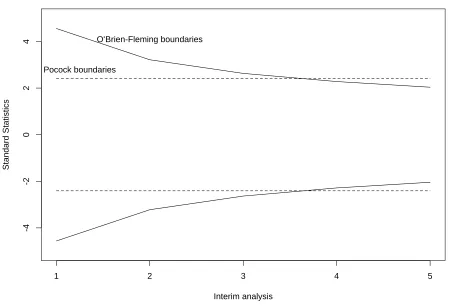
O’Brien & Fleming (1979) proposed a similar method using Pearson Chi-square tests where the test statistics are proportioned by the number of groups. Wang & Tsiatis (1987) also proposed approximately optimal one-parameter boundaries that have the form of c(α, K, ∆)·i∆−0.5, i=1, . . . , K, where c(α, K, ∆) is derived from the joint probability given in (1.1). Pocock (∆=0.5) and O’Brien-Fleming (∆=0) boundaries are included within this class of boundaries that minimize the number of subjects required for detecting significance difference at given level of significanceα, and power 1−γ. In comparison, Pocock method has boundaries fixed through all group analyses while the value of O0Brien-Fleming boundaries decreases as the num-ber of groups increases. O0Brien-Fleming method has less chance of early stopping than Pocock method since its acceptance regions are wider in the early analyses and narrower when the trial is close to completion. Thus O0Brien-Fleming method is more conservative in early stopping than Pocock method. Figure 1.1 shows the boundaries for both Pocock and O’Brien-Fleming methods when K=5, α=0.05.
or the time of analyses. This approach generalizes the previous group sequential methods so that Pocock and O0Brien-Fleming monitoring procedure become special cases. For example, the alpha-spending function for Pocock boundaries is set as
α(πi) = α·log[1 + (e−1)πi]. For O
0
Brien-Fleming spending function in two-sided test, α(πi) = 4−4Φ(Zα
4/
√π
i), where 0≤πi ≤1. The proportion π can be defined as
the fraction of information observed up to some time. For example, πi = Ki at theith
group with maximum analysis time K. It can also be approximated by the variance up to time divided by the total variance of the test.
Once a spending function is selected, the information fractions π1, π2, . . ., πM,
determine the sequential boundary valuesb1, b2, . . ., bM, under the criteria
P(|T1|< b1,|T2|< b2, . . . ,|Tj−1|< bj−1,|Tj| ≥bj|H0) =α(πj)−α(πj−1) (1.2)
where 1≤j≤M, π0=0, πM=1, α(π0)=0, α(πM)=1. The sequential boundaries b1, b2,
. . ., bM can be determined numerically using the recursive integration formula by
Armitage, McPherson & Rowe (1969). Follow the sequential process, at each interim analysis, a test statistic is compared with a stopping boundary and the action of stopping or continuing a trial will be made.
1.4
Outline
Figure 1.1: Group Sequential Boundaries for Two-sided Tests with K=5 andα=0.05: ∆ =0 and ∆ =0.5
Interim analysis
Standard Statistics
1 2 3 4 5
-4
-2
0
2
4 O’Brien-Fleming boundaries
Table 1.1: Effect of Multiple Looks at the Nominal Level K False Positive Rate
1 0.050
2 0.083
3 0.107
4 0.126
5 0.142
10 0.193
20 0.246
50 0.320
100 0.374
1000 0.530
..
. ...
Chapter 2
Nuisance Parameters Free IBM
2.1
Introduction
10% difference, or a difference from 40% to 50%, would have been diminished to 80%. In the previous example, the treatment effect was given as the difference in re-sponse rates. In some cases, investigators may be interested in assessing relative risk, that is, the ratio of response rates between treatments. For example, a treatment may be deemed important if the relative risk is 1.5 or greater (i.e. a 50% relative increase in response). Hence, if the control group response rate were 10%, then a treatment that had a response rate of 15% or greater would be clinically important, whereas, if the control group response rate were 20%, then a 30% response rate or greater would be necessary for the treatment group. When evaluating sample sizes during the de-sign stage to detect relative risk differences with some prespecified power, the intial guess for the control group response rate plays even a more critical role as deviations from the initial guess will have a greater effect on power.
For ethical as well as practical considerations, most clinical trials are designed with formal sequential stopping rules. That is, the data from a clinical trial are monitored periodically, usually by an external data monitoring board, and, if the treatment difference becomes sufficiently large during one of the interim analyses, then the study may be stopped. Formal sequential boundaries have been derived that dictate how large the treatment difference must be at different interim analyses before a study is stopped. These boundaries are constructed so that the overall test has the desired operating characteristics. That is, the resulting sequential test will have the desired level of significance and power to detect a clinically important treatment difference. Issues regarding the effect on power, of misspecifying the nuisance parameter during the design stage, are similar to those discussed earlier for the fixed sample procedure. However, when data are monitored periodically, the parameters in the model can be estimated with the available data and if these estimates are sufficiently far from the values used in the design stage, then the investigators have the ability to alter the design; i.e. adaptively increase or decease the sample size. It is the feasibility of this strategy that we will investigate in this paper.
difference (usually parametrized through a single parameter) is directly related to the Fisher Information available in the data for that parameter. Consequently, a test will have the desired power to detect a clinically important difference, if the necessary information were available at the end of the study, independent of the nuisance pa-rameters. Since the Fisher Information can be estimated by the observed information, we suggest monitoring a study using the observed information rather than the sample size. Also, since for most estimators of treatment difference, the observed information and the standard error of the parameter estimate of treatment difference are related to each other, this means that we would continue monitoring a study until the stan-dard error becomes sufficiently small. Such a strategy may necessitate changing the sample size from that initially guessed during the design stage. This would be the case if the parameters used in designing the study differed from the truth.
these three scenarios and tables of results on power and type I error are given in 2.3. Finally, we give an account of summary in 2.4.
2.2
Information-based Monitoring in Group
Se-quential Studies
The general theory for information-based monitoring has been described in detail by Sharfstein & Tsiatis (1997). In this section, we recap the steps for implementing this in a group sequential study which is generalized by the use of a type I error spending function (Lan & DeMets 1983) fit for calculating O’Brien-Fleming bound-aries.
As always, we posit a statistical model for our data in terms of parameters (β, θ), where β denotes the parameter of interest. For our problem, the parameter β will denote treatment difference, which we take to be single valued, and θ will denote a vector of nuisance parameters necessary to adequately describe the probability distribution of the data. We will focus on testing the null hypothesis of no treatment difference, usually parametrized as H0 :β = 0, against a two-sided alternative β 6= 0.
The clinically important treatment difference will be denoted by βA. That is, if, in
truth, β ≥ βA, then we would want to detect such a difference with power at least
equal to 1− γ using a test at the α level of significance. We wish to emphasize that the manner in which we choose to parameterize the problem has important implications. For example, when we were comparing dichotomous response rates between two treatments, we realized that for some studies the interest might focus on detecting absolute differences, whereas, for other studies relative risk might be important. The choice for the parameter of treatment difference β, e.g. absolute difference or relative risk, implies that the clinically important difference, β = βA,
to characterize treatment difference, whether it be absolute difference, relative risk, relative odds, or some other more appropriate measure of treatment difference.
We will consider tests that are efficient such as Wald tests, score tests, or likelihood ratio tests. For concreteness, let us consider the level α (two-sided) Wald test that rejects the null hypothesis when the statisticW = ˆβ/se( ˆβ) exceeds, in absolute value,
Zα/2, where ˆβ denotes the maximum likelihood estimator for β, se( ˆβ) denotes the
standard error of the estimator, and Zx denotes the (1−x)th quantile of a standard
normal distribution.
The Fisher Information matrix is defined as the expected value of minus the Hessian (i.e. matrix of second partial derivatives with respect to all the parameters) of the log likelihood. Under the usual regularity conditions, the asymptotic variance of the maximum likelihood estimators ( ˆβ,θˆ) is equal to the inverse of the information matrix. The asymptotic variance for ˆβ is the corresponding element on the diagonal of the inverse of the information matrix. The Fisher Information for the parameterβ
is defined as the inverse of the asymptotic variance for ˆβ. If a single test of the null hypothesis were conducted using the levelα Wald test, then by standard asymptotic theory, one could show that the information forβ, denoted by I, necessary to detect the clinically important treatment difference βA, with power 1−γ, must equal
I = Z
α
2 +Zγ
βA
!2
.
This value of information is independent of the nuisance parameters θ, although the nuisance parameters come into play in the definition of the information. The key point is that Fisher Information can be estimated using the data. In fact, the standard error of ˆβ is generally obtained from the observed information matrix, which estimates the Fisher Information matrix. Consequently, se−2( ˆβ) can be used as an estimate for the
information I. This suggests that the desired power of a level α Wald test, to detect a clinically important difference, would be achieved when
se−2( ˆβ) = Z
α
2 +Zγ
βA
!2
.
If the data are to be monitored periodically, say, at times t1, . . . , tK, then Wald
these test statistics as W(tj), j = 1, . . . , K. A group sequential test would reject the
null hypothesis and stop the study at the first time tj for which |W(tj)| ≥ cj, j =
1, . . . , K, where the boundary values cj are chosen so that the group sequential tests
have the appropriate operating characteristics. Namely, the values cj must satisfy the
following equalities:
1−Pβ=0{
K
\
j=1
|W(tj)|< cj}=α
and
Pβ=βA{
K
\
j=1
|W(tj)|< cj}=γ.
In order to derive such group-sequential boundaries that satisfy the above equalities we must be able to characerize the joint distribution of the sequentially computed Wald test statistics {W(t1), . . . , W(tK)}. The key result that allows us to compute
such boundaries in terms of Fisher Information, comes from the general theorem given by Sharfstein et al. (1997), which may be stated as follows:
Theorem 1. If βˆ is an efficient estimate of β then, regardless of the model generating the data, the asymptotic joint distribution of the sequentially computed
K-dimensional statistic{W(t1), . . . , W(tK)} is multivariate normal with mean vector
β{I(t1)1/2, . . . , I(tK)1/2}
and K×K covariance matrix, whose (j, k)th element, j ≤k, is given by
"
I(tj)
I(tk)
#1/2
j, k = 1, . . . , K,
where I(tj) denotes the Fisher Information at time tj.
We notice from the above theorem that the joint distribution is completely char-acterized by the parameter β and the Fisher Information available at the interim times. Different stategies for deriving sequential boundaries have been suggested in the literature. A class of boundaries given by Wang & Tsiatis (1987) used power functions. Namely, the boundaries cj were chosen to be proportional to I(tj)∆−.5.
equalities above necessary for the level and power of the test to be respected. When the power ∆ = 0, the resulting boundaries are similar to those originally proposed by O’Brien & Fleming (1979) and we will refer to such boundaries as O’Brien-Fleming boundaries. Another popular class of boundaries is when ∆ =.5. These are similar to boundaries suggested by Pocock (1977). It has become standard practice in clin-ical trials to use O’Brien-Fleming type boundaries. Therefore, we will restrict our numerical studies to these boundaries only. It is often convenient to characterize the maximum information M I, necessary to have power 1 −γ to detect the clinically important difference βA, as
M I = Z
α
2 +Zγ
βA
!2
IF,
where IF, defined as the inflation factor, repesents the relative increase in the in-formation necessary for a group sequential test to achieve the same power as a fixed sample test. This is a useful construct since it is often the case that IF remains relatively stable for certain classes of group-sequential boundaries. For example, it is shown in Wang & Tsiatis (1987) that anIF of 1.03 is associated with O’Brien-Fleming boundaries that are monitored at least five times.
In practice, the information at the times of analysis are not generally known in advance. Lan & DeMets (1983) suggested that one specify a spending function that dictates the amount of the significance level to be used as a funtion of the maximum information, with the constraint that all the significance level α be used at the end of the study, i.e. whenI(tK) =M I. By so doing, the boundary values can be computed
adaptively at the time of an interim analysis,tj, by estimating the Fisher Information
using se−2( ˆβ(tj)). Spending functions that result in O’Brien-Fleming and Pocock type
boundaries are given by Lan & DeMets (1983).
At each interim analysis time in a group sequential study, the information I(t) is estimated by the inverse sample variance of the parameter estimator se−2( ˆβ(t)), where
ˆ
structure that only depends on the information at each of the interim analyses. In a maximum information trial, a study is terminated when a test statistic exceeds the stopping boundary or the maximum information is attained, i.e. se−2( ˆβ) = MI.
Information-based monitoring (IBM) is free of nuisance parameters in the sense that the monitoring number, se−2( ˆβ), uses only data–indicated nuisance parameter
values and does not involve any initially guessed values. Therefore, with IBM we can obtain robust values of power over any set of nuisance parameters given a specified value of interest. For the example mentioned in 2.1, the primary interest is 10% difference between the two response rates. The information number at each time is estimated by the inverse sample variance, which involves only observed sample response rates and sample sizes at the time. Therefore, the test should obtain a 90% power whether the potential set of response rates is (20%, 30%) or (50%, 40%).
To demonstrate our point numerically, in the next section we will show simulation results of power and significance level of tests also on other types of interest such as log ratio or logit of the two response rates. We adopt the standard assumption that subjects enroll in a study according to a Poisson process with a pre-specified rate. And the outcome of interest are all observed and relatively soon so that no censoring occurrs.
2.3
Simulation Studies
We first give a general definition on the example of comparing two treatment responses. Since individual responses are independent and dichotomous, the number of responses for treatment i are binomially distributed with a response probability
πi, where i = 1,2. The test is cast as H0 : β = 0 vs. H1 : β = βA, where β is the
difference of the two response rates, π1, π2; and βA is the interest that is considered
clinically important. We chose three common relationships of response rates for the identification of βA:
1. The original interest in response difference. βA=π1−π2.
2. Log ratio of response rates. βA=log ππ1
3. Log odds ratio (logit) of response rates. βA= log
π1
1−π1
π2
1−π2
.
To emphasize that information-based group sequential tests all show 90% power under 0.05 significance level regardless of the value (π1,π2), let’s assignπ2to be 0.1, 0.2, 0.3,
0.4, or 0.5. In order to make comparisons, we accommodate the value of π1 and βA
such that at least one pair of (π1, π2) is equal in each case of interest. To illustrate this,
let the pair of matching equality be (0.4, 0.3). Then for case 1, βA= 0.4−0.3 = 0.1
and for π2 = 0.1, 0.2, 0.4, 0.5, π1 is computed byπ1 =π2+βA which is 0.2, 0.3, 0.5,
and 0.6, accordingly. For case 2, with the same pair, βA = 0.29 and π1 is calculated
based on log ratio function with π2 value known. Similarly for case 3. Repeat the
steps again for another matching pair (0.35, 0.3) to find the values of βA and π1 for
each fixed π2. The complete value of π1 and π2 for both matching pairs and for all
cases are listed on Table 2.2 and 2.3.
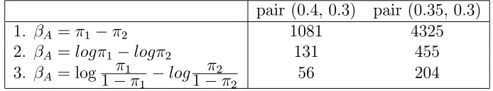
In data simulations, we assume that patient entry time is a Poisson process with total entry of 100 patients per year. The treatment indicator is a uniform (0,1) random variable, each patient having 50% chance of receiving either treatment. Each case of interest produces a different number of MI since the value of βA varies. Below
is a table of all MI numbers in all three cases for both matching pairs. For 8000
Table 2.1: MI values in all 3 cases of interests for both matching pairs. pair (0.4, 0.3) pair (0.35, 0.3)
1. βA =π1−π2 1081 4325
2. βA =logπ1−logπ2 131 455
3. βA = log1−π1π
1 −log
π2
1−π2 56 204
simulations, we averaged the number of tests rejected under the null hypothesis or under the alternative hypothesis, and also computed the average sample size (ASN). The simulation results are displayed in Table 2.2 and 2.3 as well.
We will first look at the results of case 1, interest in response differences, from Table 2.2. For the nuisance parameter set (π1,π2)=(0.3, 0.2), simulated tests give 90%
the number 783 in a fixed sample study in§1. This is one of the benefits in employing group sequential methods. For the same interest in detecting 10% difference, given (π1, π2)=(0.5, 0.4), we can see clearly that the tests obtain the same power. The
reason behind it is that rather than using total sample size as a criterion to end a study, in information-based monitoring a study ends if MI is exhausted. For the same value of interest MI stays the same. Thus a test would be expected to maintain the same power. We find the same conclusions for other interests in testing log ratio and logit of the response rates. Table 2.3 shows that detecting smaller values of interest requires larger sample sizes. For nuisance parameter values of (0.35, 0.3), tests for all three cases of interest are equivalent and thus require similar number of subjects.
2.4
Summary
Conventional statistical tests inquire a total sample size that depends on poten-tially unreliable values of nuisance parameters. This paper suggested monitoring a trial from a different angle using Fisher Information and MI number. Under a correct model assumption, an information-based monitoring study maintains expected power under a significance level regardless of the values of nuisance parameter sets, provided that the single hypothesis parameter of interest can be estimated efficiently and the alternative value of interest is preset. The idea is simulated via a simple scenario of comparing dichotomous responses among two treatments. Generally, information-based monitoring procedure is applicable to any type of model for any type of group sequential study given necessary conditions.
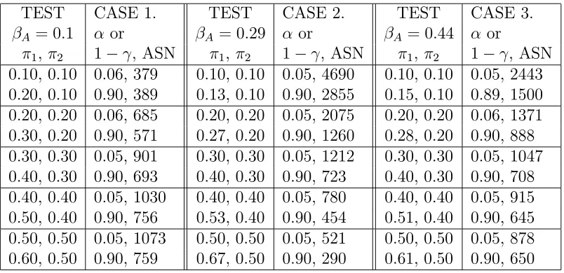
Table 2.2: Simulation results on 3 cases of parameter interests. Case1: response difference, Case2: log ratio, Case3: logit. The matching pair is (0.4, 0.3). α, 1−γ
are the computed type I error and power. ASN is the averaged sample size over 8000 simulations.
TEST CASE 1. TEST CASE 2. TEST CASE 3.
βA= 0.1 α or βA= 0.29 α or βA= 0.44 α or
π1, π2 1−γ, ASN π1, π2 1−γ, ASN π1, π2 1−γ, ASN
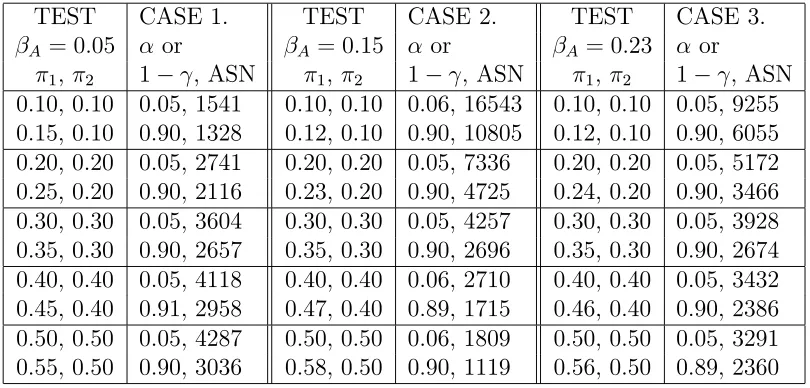
Table 2.3: Simulation results on 3 cases of parameter interests. Case1: response difference, Case2: log ratio, Case3: logit. The matching pair is (0.35, 0.3). α, 1−γ
are the computed type I error and power. ASN is the averaged sample sizes over 8000 simulations.
TEST CASE 1. TEST CASE 2. TEST CASE 3.
βA= 0.05 α or βA= 0.15 α or βA= 0.23 α or
π1, π2 1−γ, ASN π1, π2 1−γ, ASN π1, π2 1−γ, ASN
Chapter 3
IBM with Lagged or Censored
Data
3.1
Introduction
The use of sequential methods in clinical trials is now fairly common, and there is methodology and software available for their implementation. Specifically, information-based methods (Lan & Zucker 1993, Sharfstein & Tsiatis 1997) coupled with the use of alpha-spending functions (Lan & DeMets 1983) allow a flexible and unified approach for sequential monitoring of clinical trials.
clinical trial such as timing of clinic visits. The lag time may be due to a complicated combination of all of the above factors. Regardless of the exact cause, the lag time itself is of no scientific interest, but merely a factor that needs to be taken into account when inference is made from the data on response rate.
Lag may also be considered as censored at an interim time of analysis. The consequence is that the data that are actually available to the statistical center at any point in time may not be representative of the results that will eventually be available. Some lagged data may actually not be observed by the time a trial ends. In other words, the interim data may be biased in some way. For example, if information on responders came into the statistical center more quickly on the average than it did for nonresponders, then it would appear at an interim analysis as if the response rate was higher than it would be when all the data are complete. Also if the distribution of lag times was differential both by treatment and response status, then, even if the response rates were equal for two treatments, it would appear that there is a difference at an interim analysis.
There are several standard ways of dealing with this type of incomplete data. A naive way is to ignore the problem and conduct the statistical analysis with the available data. Alternatively, the analysis may be limited to those patients who entered the trial early enough to guarantee that their data were complete by the analysis time (this assumes that there is a maximum possible lag time). The results of this limited analysis should be unbiased. The problem with this method, however, is that it discards the information on some patients whose data are available, and thereby reduces the power of the analysis to detect a treatment difference. We propose a general methodology for analyzing all the available data, while still taking into account the effect of lag time. This is accomplished by considering weighted tests and estimators.
test statistics and estimators at the different monitoring times. As we illustrate in 3.3, the test statistics that we propose may be represented as stochastic integrals of counting process martingales. This representation, together with the powerful machinery developed for such processes, will enable us to derive the joint sequential distribution in 3.4. This will then allow us to compute stopping boundaries that preserve the desired operating characteristics by using information-based methods and alpha-spending functions. In 3.5, we applied the results derived from previous sections to an example of comparing two response rates. In 3.6, we performed simulations on data with dichotomous responses to demonstrate that our proposed inverse weighted estimator is consistent and requires fewer individuals entered into a study than the other two commonly used estimators. Finally the conclusions and future approach for the study of efficiency in 3.7.
3.2
Notation
Before going into specific details, we first introduce some notation. For individual
i, the outcome variable of interest will be denoted by Yi. There is a follow-up time,
Ti, that is necessary before the variable of interest is determined. Follow-up time is
measured from patient entry and is referred to as patient time. The data that are collected over patient time will be denoted by {Zi(u), u≤ Ti}, where Zi(u) denoted
the data available at timeu. For example, for objective response of cancer patients on a given treatment, Ti represents the time that the ith patient undergoes treatment,
Zi(u) represents tumor size if it is measured at time u, and an objective response, Yi,
may be defined as the indicator of whether the minimum value of Zi(u) at measured
values of (u≤Ti :Zi(u)≥0) is less than .5 timesZi(0). Ultimately, we are interested
in making inference regarding the outcome variable Yi.
With complete follow-up, we would be able to calculate the outcome variable
Yi, on all patients and be able to use standard statistical techniques for inference.
However, in many instances, we will not be able to observe the entire data history
{Zi(u), u≤Ti}due to right censoring. Censoring may result from incomplete
censoring, as the reason for censoring does not involve patient choice. In contrast, censoring may occur when a patient withdraws from the study and data on that individual are no longer collected. To accommodate censoring, we define a time to censoring as a positive random variable Ci. For a sample of npatients, the data,
which include the possibility of being censored, can be described for theith individual by Vi = min(Ti, Ci), ∆i = I(Ti ≤ Ci), and ZiH(Vi), i = 1, . . . , n, where I(·) is the
indicator function, ZH
i (x) denotes the history of the Z process for the ith individual
up to time x; that is, ZH
i (x) = {Zi(u), u ≤ x}. For practical purpose, we need to
restrict the time we evaluate each individual up to time L. That is, entry time Ti is
the minimum of the time from treatment initiation to outcome observed or L.
3.3
A Consistent Estimator And Its Martingale
Structure
Our aim is to estimate the mean of outcome interest Y when the history of data is subject to right censoring. The kernel of the methodology is based on the use of the inverse selection probability weighted estimator. To motivate this estimator, we note that with complete information for each individual, an obvious estimator for the ex-pected value ofY, which we denoted byµY, isn−1Pni=1Yi. With censoring, there is a
potential censoring timeCi, which is assumed to be independent of the data-collection
process as well as of the time Ti. Let the distribution function of the censoring time
be given by 1−K(u), whereK(u) = P(C > u). The data-collection process would be censored ifCi < Ti. Therefore, at the time of ascertainment Ti, theith individual has
a probability K(Ti) of not being censored. Therefore, each person who has complete
information (i.e., uncensored) represents, on average, 1/K(Ti) individuals who might
have been censored. Hence, a weighted estimator using only uncensored individuals, i.e., complete cases, is given by n−1Pni=1 ∆iYi
K(Ti), where ∆i =I(Ti ≤Ci). That this is
an unbiased estimator of µY is a consequence of the following equality:
E ( 1 n n X i=1
∆iYi
K(Ti)
) = E " E ( 1 n n X i=1
∆iYi
K(Ti)
Ti, ZiH(Ti)
= E " 1 n n X i=1 Yi
K(Ti)
E{I(Ci ≥Ti)|Ti, ZiH(Ti)}
#
= E 1 n n X i=1 Yi !
=µY
Because the underlying survival distribution of censoring K(Ti) is unknown, we
pro-pose to estimate it using the Kaplan-Meier estimator (Kaplan & Meier 1958). This is done by simply reversing the roles of censoring time Ci and ascertainment time
Ti; i.e. here the time Ti censors the censoring time Ci. That is, with the data
{Vi =min(Ti, Ci),∆i, i= 1, . . . , n}, the Kaplan-Meier estimator for the distribution
of the censoring timeCi is defined by
ˆ
K(t) = Y
u<t
(
1− dN
c(u)
Y(u)
)
,
where Nc(u) =Pin=1I(Vi ≤u,∆i = 0), and Y(u) =Pni=1I(Vi ≥ u). The probability
weighted complete-case estimator is defined as
ˆ
µW T =
1
n
n
X
i=1
∆iYi
ˆ
K(Ti)
.
This estimator is similar to that used by Zhao & Tsiatis (1997) to find a consistent estimator for the distribution for Quality-Adjusted Life. Consequently, consistency and asymptotic normality would follow exactly as outlined in that paper.
For our problem, we let the filtration F(u) be the set of σ-algebras generated by σ{I(Ci ≤ t), t ≤ u;Ti, Zi(x),0 ≤ x < ∞, i = 1, . . . , n}, which is the increasing
information derived by the entire data process, including ascertainment times for all individuals together with the censoring times that are observed up to time u. Although this is not the usual filtration used for censored survival problems, we find that choosing an appropriate filtration is often key to being able to solve problems that involve censoring. Because our methodology depends on estimating the distribution of censoring rather than the distribution of failure times, we will use a counting process that counts the number of individuals censored over time instead of counting the number of uncensored events. Therefore, we consider the martingale process
Mic(u), which can be written as Mic(u) = Nic(u)−R0uλc(t)Yi(t)dt, where Nic(u) =
censoring distribution. We also define Mc(u) = PMic(u), Nc(u) = PNic(u) and
Y(u) = PYi(u).
Using some well-known martingale integral equations, the probability weighted estimator can be expanded as
n1/2(ˆµW T−µY) =n−1/2 n
X
i=1
(Yi−µ)−n−1/2 n
X
i=1
Z L
0
dMic(u)
K(u) {Yi−G(Y, u)}+oP(1) (3.1) where
G(Y, u) = 1
S(u)E{YiI(Ti ≥u)},
S(u) = P(T > u),
and oP(1) is a term that converges in probability to zero as the sample size increase.
SinceYiisF(0) measurable, the two terms in (3.1) are uncorrelated and we use the
result of covariance structure of martingale process, the variance of n1/2(ˆµ
W T −µY)
is equal to
var(Yi−µ) +
Z L
0 {
G(Yi2, u)−G2(Yi, u)}S(u)
λc(u)
K(u)du (3.2) The detailed derivation of (3.1) and (3.2) is shown in Appendix A.
For large samples, the martingale version of central limit theorem (Fleming & Harrington 1991) can be used to show that ˆµW T is consistent and asymptotically
normal, and that the asymptotic variance of n1/2(ˆµW T −µY) can be estimated by
1 n " 1 n n X i=1
∆i(Yi−µˆW T)2
ˆ
K(Ti)
+ 1
n
Z L
0
dNc(u) ˆ
K(u) { ˆ
G(Y2, u)−Gˆ(Y, u)}
#
(3.3)
The second peice of the estimate is derived by taking the Nelson estimatordNc(u)/Y(u) for λcdu,
the Kaplan-Meier estimators ˆK(u) and ˆS(u) forK(u) andS(u), and ˆG(Yi, u), ˆG(Yi2, u)
for G(Yi, u),G(Yi2, u); where
ˆ
G(Y, u) = 1
n
1 ˆ
S(u)
n
X
i=1
∆iYiI(Ti ≥u)
ˆ
K(Ti)
linear; that is, the estimator minus the estimand can be approximated by a sum of identically and independently distributed mean zero random variables, which are re-ferred to as influence functions. The asymptotic properties for such asymptotically linear estimators are therefore directly related to their influence function. In particu-lar, the asymptotic variance of the estimator is the variance of the influence function for a single observation.
3.4
Sequential Joint Distribution with Censored
Data
The problems associated with incomplete follow-up are most pronounced during interim analyses when the trial participants have varying amounts of follow-up and completeness. In most clinical trials sequential stopping rules are used to stop a study early if treatment difference become sufficiently large during an interim analysis. In order to develop such sequential stopping rules with desired operating characteristics (i.e., type I and type II errors) we must be able to characterize the joint distribution of relevant test statistics and estimators over calendar time. In the previous section, we described a comprehensive approach for testing and estimating at a single analysis time with incomplete follow-up data. We will generalize these results in order to derive the joint distribution of the sequentially computed tests or estimates. Once we have derived the joint sequential distribution we will then be able to construct stopping boundaries for group sequential tests that have the desired type I error and power. The key to deriving the joint sequential distribution is to identify the influence function of the estimators at the interim monitoring times. The joint distribution of the sequentially computed estimators would then be asymptotically normal with the correlation structure of their corresponding influence functions.
To accommodate interim monitoring, we define a random variable Ei to denote
as a realization of a sequence of independent random vectors {Yi, Ti, ZiH(Ti), Ei},
i= 1, . . . , n. It is important to distinguish between two different time scales, patient time versus calendar time. Entry into the study occurs at calendar time as does the analysis of the data at different interim times. However, the time Ti and the process
ZH
i (x) are measured from the time patient i enters into the study. The variable Ei
will be assumed to be independent of {Yi, Ti, ZiH(Ti)}. In this representation, n is
the total number of patients that will eventually enter the trial at random times Ei,
i = 1, . . . , n, during a fixed accrual period. Asymptotic theory, which is predicated on letting n go to infinity, is a consequence of an increasing number of individuals arriving during the accrual period. This type of asymptotic theory most closely represents the situation in a large scale clinical trial, and has been used to derive the sequential theory for clinical trials based on calendar time, (Tsiatis 1981,1982,1995). Of course, at any time t, the analysis is limited to only those n(t) = Pin=1I(Ei ≤ t)
individuals who entered the study prior to that time. Also, if the analysis is conducted at calendar tiemt, then an individual would have incomplete follow-up (i.e, censored data) if Ti ≤t−Ei. We therefore define the censoring variable at analysis time t as
Cti=t−Ei.
In many instances, the research hypothesis under investigation can be cast as a hypothesis testing question involving a single scalar parameter β. For example, if tumor response is the primary outcome, β may denote the difference in the response rates between two treatments. The model is usually parametrized so that the primary question being tested is the null hypothesisH0 :β = 0. In a group-sequential analysis,
the null hypothesis is tested at different interim times with the possibility of early stopping if the test statistic becomes sufficiently large at any of the analyses. We will focus on the use of a Wald test for this purpose, although a parallel development could also be used for score tests. Towards that end, we denoted the estimator for a parameter of interest calculated using only the data available up to calendar time t, by ˆβt. Most estimators are asymptotically linear; that is, they can be written as
n1/2( ˆβt−β0) =n−1/2
n
X
i=1
φt(Yi, Ti, ZiH(·), Ei)I(Ei ≤t) +op(1),
influence function of ˆβt. By the central limit theorem, the asymptotic distribution
of n1/2( ˆβ
t−β0) is normally distributed with mean zero and variance equal to the
variance of φt(Yi, Ti, ZiH(·), Ei)I(Ei ≤t).
If the data are monitored at interim times t1, . . . , tK, then the joint distribution
of
n1/2( ˆβt1 −β0), . . . , n
1/2( ˆβ
tK −β0)
equivalent to the joint distribution of their corresponding influence functions
n−1/2
n
X
i=1
φt1(Yi, Ti, Z
H
i (·), Ei)I(Ei ≤t1), . . . , n−1/2
n
X
i=1
φtK(Yi, Ti, Z
H
i (·), Ei)I(Ei ≤tK)(3.4)
By the multivariate central limit theorem, the K-dimensional random vector (3.4) converges to a multivariate normal random vector with mean zero and K×K covari-ance matrix Ω with elements
Ωjk = cov[φtj(Yi, Ti, Z
H
i (·), Ei)I(Ei ≤tj), φtk(Yi, Ti, Z
H
i (·), Ei)I(Ei ≤tk)]; (3.5)
j, k = 1, . . . , K.
3.5
Application in Comparing Two Response Rates
As an example, we illustrate how this method would be applied if we wanted to evaluated the sequential distribution of an estimator for response rate with incomplete follow-up. Let θ denote the probability of response. This would correspond to the E(Y), where Y is a dichotomous indicator of response. Use of the inverse selection probability weighted estimator for θ at calendar time t would result in
ˆ
θt =n−1(t) n
X
i=1
∆ti
ˆ
Kt(Ti)
YiI(Ei ≤t)
where ∆ti = I(Cti ≥ Tti), Cti = t−Ei, and ˆKt(u) is the Kaplan-Meier estimator
for Cti using the censored data min(Ti, Cti) for {i : Ei ≤ t}. Using the martingale
toKt(u) = P(Cti ≥u)/π(t) we may write
n1/2(ˆθt−θ) = n−1/2 n
X
i=1
π(t)−1{Yi−θ}I(Ei ≤t)
−n−1/2
n
X
i=1
π(t)−1
Z dMCti(u) Kt(u)
{Yi−G(Y, u)}+op(1),
where L is the maximum time to evaluation. This implies that the influence function for ˆθt is given by
φt(Yi, Ti, ZiH(.), Ei)I(Ei ≤t) = π(t)−1{Yi−θ}I(Ei ≤t)
−π(t)−1
Z L
0
dMCti(u) Kt(u)
{Yi−G(Y, u)} (3.6)
From (3.4), the asymptotic joint distribution of the estimator forθevaluated at times
t1, . . . , tK is a multivariate normal with mean zero and covariance matrix given by
(3.5).
It remains now to evaluate the covariance structure. It suffices to consider the influence function at two arbitrary points s < t; that is, we wish to compute
covφs(Yi, Ti, ZiH(.), Ei)I(Ei ≤s), φt(Yi, Ti, ZiH(.), Ei)I(Ei ≤t)
The important useful feature is that the influence functionis is expressed as a stochas-tic integral of a martingale process. If we additionally note that the martingale process
MCsi(u) = MCti(u+ (t−s)), then the influence functions at times s and t may be
written as stochastic integrals with respect to a common martingale process,MCti(u).
Invoking some simplifying formula for the covariance of stochastic integrals with re-spect to the same counting process, then after some algebra we obtain
covφs(Yi, Ti, ZiH(.), Ei)I(Ei ≤s), φt(Yi, Ti, ZiH(.), Ei)I(Ei ≤t)
= varφt(Yi, Ti, ZiH(.), Ei)I(Ei ≤t)
(3.7)
A detailed proof is shown in Appendix B.
based design and monitoring” for this problem. Statistical information is equated with the inverse of the variance of the estimator, which grows over time as we accumulate more data. The group-sequential stopping rules can then be constructed according to the methods proposed by Lan & DeMets (1983), whereby an alpha-spending function is specified that dictates how much of the significance level can be used as a function of the statistical information. This in turn may be translated into corresponding stopping boundaries that preserve the overall type I and type II error.
One immediate consequence of the above result involves testing the equality of response rates between two treatments. The test would be based on the difference between the treatment specific estimates of response rates computed above. A simple calculation shows that the difference of the two estimators of responses, calculated sequentially over calendar time, also has the independent increments structure. The monitoring process for this problem may then be carried out routinely.
3.6
Simulations
A numerical simulation is performed to test the equality of response rates between two treatments, A, B, with information-based monitoring procedure. Let πi denote
the probability of response for each treatment. The null hypothesis is H0 : θ =
πA−πB = 0. A set of data are generated under the assumption that individual entry
time Ei follows a Poisson process with total entry of 500 subjects per time unit. The
outcome of response Y is a dichotomous variable. And individual response or non-response time to each treatment is exponentially distributed with parameterλvaried. That is, the lag time TAi for individualito respond to treatment A has λA= 1 while
for non-responding to treatment A, the parameter λN
A = 2. Similarly for treatment
B, the lag time TBi follows exponential distributions with λB = 2 for responders and
λNB = 1 for nonresponders. The rates of information available at time t not only vary by response time but also by treatments. This design signifies the bias that is caused by incomplete follow-up in a trial. The data are divided into groups according to treatments. LetYli be the response outcome of an individual taking treatment l, l=
taking treatment l; ∆tli=I(Cti ≥Tli), where Cti =t−Ei, the censored time.
Before carrying out the information-based monitoring procedure, we will first show the estimate and and asymptotic variance for each method. Naively, we could ignore the problem of incomlete follow-up and use the data available at time t to estimate the probability of responses. The naive estimator is denoted by θN Vˆ .
ˆ
θN V = ˆπAN V −πˆBN V =
1
nA(t) nXA(t)
i=1
YAi∆tAi −
1
nB(t) nXB(t)
i=1
YBi∆tBi,
where ˆπN VA = 1
nA(t) nXA(t)
i=1
YAi∆tAi, πˆBN V =
1
nB(t) nXB(t)
i=1
YBi∆tBi.
And the asymptotic variance for ˆθN V is computed impirically. That is,
ˆ
Var(ˆθN V) =
1
nA(t)
1
nA(t)−1 nXA(t)
i=1
{I(Ei ≤t)I(Trt =A)−πˆN VA }
2
+ 1
nB(t)
1
nB(t)−1 nXB(t)
i=1
{I(Ei ≤t)I(Trt =B)−πˆBN V}2
For a desired 5% type I error and 90% power, the naive estimate is expected to have a much higher risk of making a type I error in a trial.
To take into account of the lag time variable, we assume the maximum lag time to be 1 time unit. That is, at time t the information before time (t− 1) will be complete. Thus at each interim analysis, we draw inference using data only one unit before time. The maximum lag time estimator
ˆ
θM L = ˆπAM L−ˆπ M L B =
1
nA(t−1)
nAX(t−1)
i=1
YAi−
1
nB(t−1)
nBX(t−1)
i=1
YBi,
where ˆπM LA = 1
nA(t−1)
nAX(t−1)
i=1
YAi, πˆM LB =
1
nB(t−1)
nBX(t−1)
i=1
YBi.
And the asymptotic variance
ˆ
Var(ˆθM L) =
ˆ
πM L
A (1−πˆAM L)
nA(t−1)
+πˆ
M L
B (1−πˆBM L)
nB(t−1)
ˆ
θM L is a consistent estimate. But since this method discards partial information
The inverse weighted estimator for the probability of response for each treatment group is
ˆ
πlIW = 1
nl(t) nXl(t)
i=1
∆tliYli
ˆ
Ktl(Tli)
, l=A, B.
Thus the inverse weighted estimator for θ is
ˆ
θIW =
1
nA(t) nXA(t)
i=1
∆tAiYAi
ˆ
KtA(TAi)
+ 1
nB(t) nXB(t)
i=1
∆tBiYBi
ˆ
KtB(TBi)
The asymptotic variance of ˆθIW is the sum of the asymptotic variance based on
(3.3) under each treatment group . Simulations should demonstrate that this method maintains the desired type I and type II errors, and reduces the number of individuals required in a trial than the maximum lag time method.
With the estimated variances, we can compute the proportion of information, I/MI, at each interim time where I is the inverse variance and MI is the maximum number. A study ends when a clinical difference is identified or when all information is exhausted, i.e. I/MI=1. To futher enhance the phenomena that incomplete follow-up may lead to biased results in the early interim analysis, we choose the alpha-spending function that resembles the Pocock boundary which is more optimistic in early stopping. For the probability of response ranging from 0.1 to 0.5, we would like to detect a 0.05 difference under the alternative hypothesis. Given the expected 5% level of significance and 90% power, the standard error under 1000 simulations for each hypothesis is equal to
q
0.05(1−0.05)
1000 = 0.006892. Therefore the simulation type I
error should be within the interval of (0.043, 0.057), and power within (0.893, 0.907). We also give the average sample number (ASN) for 1000 simulations to compare on all three methods. See Table 1.
two methods show lower than expected because Pocock boundaries are more liberate in stopping in the early stage of a trial, therefore increasing the chance of making type II error. For the use of O’Brien–Fleming boundaries, The powers obtained from the maximum lag and inverse weighted methods are indeed inside in expected range.
3.7
Future Approach
Table 3.1: Simulation result on 3 parameter estimators with incomplete follow-up data. Pocock boundaries are used.
Test Naive Max. lag time Inverse weighted
πA,πB α/(1−γ), ASN α/(1−γ), ASN α/(1−γ), ASN
0.10, 0.10 0.18, 2012 0.05, 2332 0.05, 2151
0.15, 0.10 0.90, 1812 0.90, 1565
0.20, 0.20 0.24, 3117 0.07, 3663 0.05, 3568
0.25, 0.20 0.90, 2514 0.90, 2307
0.30, 0.30 0.21, 4181 0.06, 4634 0.05, 4488
0.35, 0.30 0.90, 2978 0.90, 2796
0.40, 0.40 0.22, 4723 0.05, 5224 0.05, 5103
0.45, 0.40 0.90, 3241 0.90, 3124
0.50, 0.50 0.19, 5150 0.05, 5224 0.06, 4436
Table 3.2: Simulation result on 3 parameter estimators with incomplete follow-up data. O’Brien-Fleming boundaries are used.
Test Naive Max. lag time Inverse weighted
πA,πB α/(1−γ), ASN α/(1−γ), ASN α/(1−γ), ASN
0.10, 0.10 0.13, 2119 0.05, 2219 0.06, 1834
0.15, 0.10 0.90, 1980 0.88, 1455
0.20, 0.20 0.23, 3201 0.05, 3292 0.05, 2972
0.25, 0.20 0.90, 2736 0.89, 2138
0.30, 0.30 0.14, 3144 0.05, 4159 0.06, 3793
0.35, 0.30 0.89, 3262 0.90, 2573
0.40, 0.40 0.13, 3479 0.06, 4645 0.04, 4291
0.45, 0.40 0.91, 3508 0.90, 2808
0.50, 0.50 0.11, 4765 0.05, 4806 0.05, 4436
Bibliography
Armitage, P., McPherson, C. K. & Rowe, B. C. (1969), ‘Repeated significance tests on accumulating data’, Journal of the royal statistical society132, A:235–244. Bang, H. & Tsiatis, A. A. (1999), ‘Estimating medical costs with censored data’,
Biometrika.
Fleming, T. R. & Harrington, D. P. (1991),Counting Processes and Survival Analysis, Wiley, New York.
Friedman, L. M., Furberg, C. D. & DeMets, D. L. (1998), Fundamentals of Clinical
Trials, 3rd edn, Springer, New York.
Gill, R. D. (1980),Censoring and Stochastic Integrals, Mathematisch Centrum, Am-sterdam. Mathematical Centre Tracts 124.
Jewell, N., Dietz, K. & Farewell, V., eds (1992), AIDS Epidemiology-Methodological
Issues.
Kaplan, E. L. & Meier, P. (1958), ‘Nonparametric estimation from incomplete obser-vations’, Journal of The American Statistical Association 53, 457–481.
Lan, G. K. K. & DeMets, D. L. (1983), ‘Discrete sequential boundaries for clinical trials’, Biometrika70, 659–663.
O’Brien, P. C. & Fleming, T. R. (1979), ‘A multiple testing procedure for clinical trials’, Biometrics 35, 549–556.
Pocock, S. J. (1977), ‘Group sequential methods in the design and analysis of clinical trials’, Biometrika64, 191–199.
Robins, J. M. & Rotnitzky, A. (1992), Recovery of information and adjustment for dependent censoring using surrogate markers,inJewell, Dietz & Farewell (1992), pp. 297–331.
Robins, J. M., Rotnitzky, A. & Zhao, L. P. (1994), ‘Estimation of regression coeffi-cients when some regressors are not always observed’, Journal of The American
Statistical Association 89, 846–866.
Sharfstein, D. O. & Tsiatis, A. A. (1997), ‘The use of simulation and bootstrap in information-based group sequential studies’, Statistics in medicine 17, 75–87. Sharfstein, D. O., Tsiatis, A. A. & Robins, J. M. (1997), ‘Semiparametric efficiency:
implications for the design and analysis of group sequential studies’, Journal of
the American Statistical Association 92(440), 1342–1350.
Wang, S. K. & Tsiatis, A. A. (1987), ‘Approximately optimal one-parameter bound-aries for group sequential trials’, Biometric 43, 193–199.
Appendix A.
Derivation of n1/2(ˆµ
W T −µY) and its variance
Using an identity from Robins & Rotnitzky (1992, p.313)
∆i
K(Vi)
= 1−
Z ∞
0
dMc i(u)
K(u) ,
a well-known martingale integral representation Gill (1980, p.37) that ˆ
K(t)−K(t)
K(t) =−
Z t
0
ˆ
K(u−)
K(u)
dMc(u)
Y(u) ,
where ˆK(u−) is the left-continuous version of Kaplan-Meier estimator for censoring, and also
n−1Y(u) = ˆK(u−) ˆS(u−),
where ˆS(u) is the Kaplan-Meier estimator for S(u) = P(T > u), the simple weighted estimator can be expanded as
n1/2(ˆµW T −µY) = n−1/2 n
X
i=1
∆iYi
K(Ti)
+n−1/2
n
X
i=1
∆iYi
K(Ti)
(
K(Ti)−Kˆ(Ti)
ˆ
K(Ti)
)
−n1/2µY
= n−1/2
n
X
i=1
(Yi−µ)−n−1/2 n
X
i=1
Z L
0
dMic(u)
K(u) {Yi−Gˆ(Y, u)} = n−1/2
n
X
i=1
(Yi−µ)−n−1/2 n X i=1 Z L 0 dMc i(u)
K(u) {Yi−G(Y, u)}+oP(1) (A.1)
where
G(Y, u) = 1
S(u)E{YiI(Ti ≥u)}, ˆ
G(Y, u) = 1
n
1 ˆ
S(u)
n
X
i=1
∆iYiI(Ti ≥u)
ˆ
K(Ti)
, (A.2)
and oP(1) is a term that converges in probability to zero as the sample size increase.
to
var(Yi−µ) +E
"Z L
0
{Yi−G(Y, u)}2
K2(u) λ
c(u)Y i(u)du
#
= var(Yi−µ) +E
"Z L
0 {
Yi−G(Y, u)}2I(Ti ≥u)
λc(u)
K2(u)du
#
,
where Yi(u) =I(Vi ≥u) = I(min(Ti, Ci)≥u) =I(Ti ≥u)I(Ci ≥u)
and Yi(u)
K(u) =
I(Ti ≥u)I(Ci ≥u)
P(Ci ≥u)
=I(Ti ≥u)
= var(Yi−µ) +
Z L
0 {
G(Yi2, u)−G2(Yi, u)}S(u)
λc(u)
K(u)du
Appendix B.
Proof of independent increment structure using influence functionφ of two response
rates.
Our goal is to show that
covφs(Yi, Ti, ZiH(.), Ei)I(Ei ≤s), φt(Yi, Ti, ZiH(.), Ei)I(Ei ≤t)
= varφt(Yi, Ti, ZiH(.), Ei)I(Ei ≤t)
To start with, we reform the influence functions (3.6) at the two time points and shorten the notation φt(Yi, Ti, ZiH(·), Ei) to φt, φs(Yi, Ti, ZiH(·), Ei) to φs. And note
that
dMCti(u) = dNc
i(u)−λ c
t(u)yi(u)du
= I(Cti =u, Ti ≥u)−λtc(u)I(Cti ≥u, Ti ≥u)
= hI(Cti =u)−λct(u)I(Cti ≥u)
i
I(Ti ≥u)
= dM∗Cti(u)I(T
i ≥u)
, wheredM∗Cti(u) = I(C
M∗Cti(u) is also a martingale process at the time censoring occurred.
Thus at time t,
φtI(Ei ≤t) =π(t)−1{Yi−θ}I(Ei ≤t)−π(t)−1
Z L
0
dM∗Cti(u) Kt(u) {
Yi−G(Y, u)}I(Ti ≥u)
(B.1) At time s, it can be shown following the definition that
dM∗Csi(u) =dM∗Cti(u−(t−s)) Ks(u)φ(s) = Kt(u)φ(t)
Hence,
φsI(Ei ≤s) = π(s)−1{Yi−θ}I(Ei ≤s)−π(s)−1
Z L
0
dM∗Csi(u) Ks(u)
{Yi−G(Y, u)}I(Ti ≥u)
= π(s)−1{Yi−θ}I(Ei ≤s)
−π(t)−1
Z L
0
dM∗Cti(u+ (t−s)) Kt(u+ (t−s)) {
Yi−G(Y, u)}I(Ti ≥u)
= π(s)−1{Yi−θ}I(Ei ≤s)
−π(t)−1
Z L+(t−s)
t−s
dM∗Cti(u) Kt(u) {
Yi−G(Y, u−(t−s))}I(Ti ≥u−(t−s))
(B.2)
Now to find the covariance of the influence functions at time s and t,
covφsI(Ei ≤s), φtI(Ei ≤t)
=EφsI(Ei ≤s)φtI(Ei ≤t)
−EφsI(Ei ≤s)
EφtI(Ei ≤t)
There are four cross products from EφsI(Ei ≤s)φtI(Ei ≤t)
.
• The cross product of 1st terms of (B.1)& (B.2)
Ehπ(t)−1π(s)−1{Yi−θ}2I(Ei ≤s)I(Ei ≤t)
i
=π(t)−1E{Yi−θ}2 (B.3)
Since s < t, I(Ei ≤ s)I(Ei ≤ t) = I(Ei ≤ s), Ei is independent of Yi, and
EI(Ei ≤s)
• The cross product of 1st term of (B.1) & 2nd term of (B.2)
π(t)−2E
"
{Yi−θ}I(Ei ≤t)
Z L+t−s t−s
dM∗Cti(u) Kt(u) {
Yi−G(Y, u−(t−s))}I(Ti ≥u−(t−s))
#
= π(t)−2E
"Z dM∗Cti(u)I(E
i ≤t)
Kt(u)
{Yi−θ}{Yi−G(Y, u−(t−s))}I(Ti ≥u−(t−s))
#
= π(t)−2E
"Z dM∗Cti(u) Kt(u))
{Yi−θ}{Yi−G(Y, u−(t−s))}I(Ti ≥u−(t−s))
#
(B.4)
where dM∗Cti(u)I(E
i≤t) =dM∗Cti(u).
The range [t−s, L+(t−s)] = [0, L+(t−s)]\[0,t−s). The integral from [t−s, L+(t−s)] in (B.4) is then the difference of two stochastic integrals, hence has expectation zero. Therefore, (B.4) = 0.
• The cross product of 2nd term of (B.1) & 1st term of (B.2)
π(s)−1π(t)−1E
"
{Yi−θ}I(Ei ≤s)
Z L
0
dM∗Cti(u) Kt(u)
{Yi−G(Y, u)}I(Ti ≥u)
#
=π(s)−1π(t)−1E
"Z L
0
dM∗Cti(u)I(E
i ≤s)
Kt(u) {
Yi−θ}{Yi−G(Y, u)}I(Ti ≥u)
#
(B.5)
I(Ei ≤s) = I(t−Ei ≥t−s)
dM∗Cti(u)I(E
i ≤s) =
h
I(Cti=u)−λtc(u)I(Cti ≥u)
i
I(Ei ≤s)
= I(t−Ei =u)I(t−Ei ≥t−s)−λtc(u)I(t−Ei ≥u)I(t−Ei ≥t−s)
=
I(t−Ei =u)−λct(u)I(t−Ei ≥u) , for u≥t−s
−λc
t(u)I(t−Ei ≥t−s) , for u < t−s
=
dM∗Cti(u) , foru≥t−s
−λc
t(u)I(Ei ≤s) , for u < t−s
Therefore,
(B.5) =π(s)−1π(t)−1E
"Z t−s
0
−λc
t(u)I(Ei ≤s)
Kt(u)
{Yi−θ}{Yi−G(Y, u)}I(Ti≥u)
#
+π(s)−1π(t)−1E
"Z L t−s
dM∗Cti(u) Kt(u)
{Yi−θ}{Yi−G(Y, u)}I(Ti ≥u)
#
The second item in (B.6) is the expectation of a stochastic integral from [0, L] minus the same martingale process but from [0, t−s), hence is equal to 0. For the first item we take the expectation inside the integral, since I(Ei ≤s) is
independent ofYi and E
I(Ei ≤s)
=π(s) which cancels out π(s)−1.
(B.6) = π(t)−1
Z t−s
0
−λc t(u)
Kt(u)
Eh{Yi−θ}{Yi−G(Y, u)}I(Ti ≥u)
i
= π(t)−1E
"Z t−s
0
−λc t(u)
Kt(u) {
Yi−G(Y, u)}2I(Ti ≥u)
#
(B.7)
where
Eh{Yi−θ}{Yi−G(Y, u)}I(Ti ≥u)
i
= Eh{Yi−G(Y, u) +G(Y, u)−θ}{Yi−G(Y, u)}I(Ti ≥u)
i
= Eh{Yi−G(Y, u)}2I(Ti ≥u)
i
+G(Y, u)EhYiI(Ti ≥u)
i
−G2(Y, u)S(u)
−θEhYiI(Ti ≥u)
i
+θG(Y, u)S(u) = Eh{Yi−G(Y, u)}2I(Ti ≥u)
i
,
note that G(Y, u) = 1
S(u)E{YiI(Ti ≥u)}
• The cross product of integral terms in (B.1), (B.2)
π(t)−2E
"Z L
0
dM∗Cti(u) Kt(u)
{Yi−G(Y, u)}I(Ti ≥u)
× Z L+(t−s)
t−s
dM∗Cti(u) Kt(u)
{Yi−G(Y, u−(t−s))}I(Ti ≥u−(t−s))
#
= π(t)−2E
"Z L t−s
λc
t(u)I(t−Ei ≥u)
K2
t(u)
{Yi−G(Y, u)}{Yi−G(Y, u−(t−s))}I(Ti ≥u)
#
(B.8)
This is resulted by applying the covariance structure of stochastic integrals, also
I(Ti ≥u)I(Ti ≥u−(t−s)) =I(Ti ≥u).
We again take expectation inside the integral and sinceEi is independent of Yi,
Ti, E
I(t−Ei ≥u)
=Kt(u)π(t),
(B.8) =π(t)−1
Z L t−s
λct(u)
Kt(u)
Eh{Yi−G(Y, u)}{Yi−G(Y, u−(t−s))}I(Ti ≥u)
i
= π(t)−1E
"Z L t−s
λc t(u)
Kt(u){
Yi−G(Y, u)}2I(Ti ≥u)
#
where with adding and subtracting G(Y, u) on {Yi−G(Y, u−(t−s))},
Eh{Yi−G(Y, u)}{Yi−G(Y, u−(t−s))}I(Ti ≥u)
i
=Eh{Yi−G(Y, u)}2I(Ti ≥u)
i
Now adding (B.3), (B.4), (B.7), (B.9), we obtain
EφsI(Ei ≤s)φtI(Ei ≤t)
= π(t)−1E{Yi−θ}2 + 0−π(t)−1E
"Z t−s
0
−λct(u)
Kt(u)
{Yi−G(Y, u)}2I(Ti ≥u)
#
+π(t)−1E
"Z L t−s
λct(u)
Kt(u)
{Yi−G(Y, u)}2I(Ti ≥u)
#
= π(t)−1E{Yi−θ}2 +π(t)−1E
"Z L
0
λc t(u)
Kt(u)
{Yi−G(Y, u)}2I(Ti ≥u)
#
= covφsI(Ei ≤s), φtI(Ei ≤t)
since EφsI(Ei ≤s)
= 0 =EφtI(Ei ≤t)
.
We are now left to find the variance of φtI(Ei ≤ t) and show it is equal to the
covariance above.
varφtI(Ei ≤t)
=EφtI(Ei ≤t)
2
= π(t)−1E{Yi−θ}2+π(t)−2E
"Z L
0
λct(u)I(t−Ei ≥u)
K2
t(u)
{Yi−G(Y, u)}2I(Ti ≥u)
#
= π(t)−1E{Yi−θ}2+π(t)−1E
"Z L
0
λct(u)
Kt(u)
{Yi−G(Y, u)}2I(Ti ≥u)
#
= covφsI(Ei ≤s), φtI(Ei ≤t)