Can Deep Learning Improve Genomic Prediction of Complex Human Traits?

(1)

HIGHLIGHTED ARTICLE

| GENOMIC PREDICTION

Can Deep Learning Improve Genomic Prediction of

Complex Human Traits?

Pau Bellot,*,1_{Gustavo de los Campos,}†,‡_{and Miguel Pérez-Enciso*},§,2 *Centre for Research in Agricultural Genomics (CRAG), Consejo Superior de Investigaciones Cientíﬁcas (CSIC) - Institut de Recerca i Tecnologies Agroalimentaries (IRTA) - Universitat Autònoma de Barcelona (UAB) - Universitat de Barcelona (UB) Consortium, 08193 Bellaterra, Barcelona, Spain,†Department of Epidemiology and Biostatistics, and‡Department of Statistics, Michigan State University, East Lansing, Michigan 48824, and§Institut Català de Recerca Avançada (ICREA), 08010 Barcelona, Spain ORCID IDs: 0000-0001-9503-4710 (P.B.); 0000-0001-5692-7129 (G.d.l.); 0000-0003-3524-995X (M.P.-E.)

ABSTRACTThe genetic analysis of complex traits does not escape the current excitement around artificial intelligence, including a renewed interest in“deep learning”(DL) techniques such as Multilayer Perceptrons (MLPs) and Convolutional Neural Networks (CNNs). However, the performance of DL for genomic prediction of complex human traits has not been comprehensively tested. To provide an evaluation of MLPs and CNNs, we used data from distantly related white Caucasian individuals (n100k individuals,m500k SNPs, andk= 1000) of the interim release of the UK Biobank. We analyzed a total offive phenotypes: height, bone heel mineral density, body mass index, systolic blood pressure, and waist–hip ratio, with genomic heritabilities ranging from0.20 to 0.70. After hyper-parameter optimization using a genetic algorithm, we considered several configurations, from shallow to deep learners, and compared the predictive performance of MLPs and CNNs with that of Bayesian linear regressions across sets of SNPs (from 10k to 50k) that were preselected using single-marker regression analyses. For height, a highly heritable phenotype, all methods performed similarly, al-though CNNs were slightly but consistently worse. For the rest of the phenotypes, the performance of some CNNs was comparable or slightly better than linear methods. Performance of MLPs was highly dependent on SNP set and phenotype. In all, over the range of traits evaluated in this study, CNN performance was competitive to linear models, but we did notfind any case where DL outperformed the linear model by a sizable margin. We suggest that more research is needed to adapt CNN methodology, originally motivated by image analysis, to genetic-based problems in order for CNNs to be competitive with linear models.

KEYWORDSConvolutional Neural Networks; complex traits; deep learning; genomic prediction; Multilayer Perceptrons; UK Biobank; whole-genome; Genomic Prediction regressions; GenPred

A

major challenge of modern genetics is to predict an individual’s phenotype (or disease risk) from the knowl-edge of molecular information such as genotyping arrays or even complete sequences. Applications of genomic prediction range from the assessment of disease risk in humans (e.g., de los Camposet al.2010) to breeding value prediction in ani-mal and plant breeding (e.g., Meuwissen et al.2013). Un-derstanding how DNA sequences translate into disease risk

is certainly a central problem in medicine (Lee et al.2011; Strangeret al.2011).

Genome-wide association studies (GWAS) have been used extensively to uncover variants associated with many impor-tant human traits and diseases. However, for the majority of complex human traits and diseases, GWAS-signiﬁcant SNPs explain only a small fraction of the interindividual differences in genetic risk (Maher 2008). Whole-Genome Regression (WGR), a methodology originally proposed by Meuwissen et al.(2001), can be used to confront the missing heritability problem. In a WGR, phenotypes are regressed on potentially hundreds of thousands of SNPs concurrently. This approach has been successfully adopted in plant and animal breeding (e.g., de los Camposet al. 2013), and has more recently received increased attention in the analysis and prediction of complex human traits (e.g., Yanget al.2010; Kimet al. 2017).

Manuscript received June 26, 2018; accepted for publication August 24, 2018; published Early Online August 31, 2018.

Supplemental material available at Figshare:https://doi.org/10.6084/m9.ﬁgshare. 7035866.

1_{Present address: Brainomix, 263 Banbury Road, Oxford OX2 7HN, United}

Kingdom.

2_{Corresponding author: Centre for Research in Agricultural Genomics (CRAG), ICREA,}

(2)

Most of the applications of WGRs in human genetics use linear models. These models have multiple appealing features and have proven to be effective for the prediction of com-plex traits in multiple applications. Recent developments in machine learning enable the implementation of high-dimensional regressions using nonlinear methods that have been shown to be effective in uncovering complex patterns relating inputs (SNPs in our case) and outputs (phenotypes). Among the many machine learning methods available, deep learning (DL) methods such as Multilayer Perceptrons (MLPs) have emerged as one of the most powerful pattern-recognition methods (Goodfellowet al.2016). DL has demonstrated its utility in disparate ﬁelds such as computer vision, machine translation, and automatic driving, among others. It has also been applied to genomic problems using Convolutional Neu-ral Networks (CNNs) to learn the functional activity of DNA sequences (Kelleyet al.2016), predict the effects of noncod-ing DNA (Zhou and Troyanskaya 2015), investigate the reg-ulatory role of RNA-binding proteins in alternative splicing (Alipanahi et al. 2015), or infer gene expression patterns, among others.

Shallow neural networks (NNs, e.g., single-layer net-works) have been considered for nonparametric prediction of complex traits in plant and animal breeding (Gianolaet al. 2011; González-Camachoet al.2012; Pérez-Rodríguezet al. 2012). Some of these studies suggest that NNs can achieve reasonably high prediction accuracy; however, there has not been consistent evidence indicating that NNs can outperform linear models in prediction. Perhaps most importantly, most of the available studies were based on relatively small sample sizes and limited numbers of SNPs. So far, the application of NNs for genomic prediction of complex traits has been lim-ited, with only a few studies published in animal (e.g., Okut et al.2011) and plant breeding (e.g., González-Camachoet al. 2016).

In this study, we present an application of DL for the prediction of complex human traits using data from distantly related individuals. Achieving high prediction accuracy with MLPs or CNNs requires using very large data sets for model training (TRN). Until recently, such data sets were not avail-able in human genetics. Fortunately, this situation has changed as very large biomedical data sets from biobanks become available. Here, we use data from the interim release of the UK Biobank (http://www.ukbiobank.ac.uk/), and com-pare the predictive performance of various MLPs and CNNs with commonly used linear regression methods [BayesB and Bayesian Ridge Regression (BRR)] using ﬁve complex human traits.

Materials and Methods

Data set

The UK Biobank (www.ukbiobank.ac.uk) is a prospective co-hort including half a million participants aged between 40 and 69 years who were recruited between 2006 and

2010. From the subjects whose genotypes and phenotypes were provided, we used data from those that were white Caucasians (self-identified and confirmed with SNP-derived principle components) and were distantly related (genomic relationships,0.03). For comparison purposes, we use the same data set and the same TRN testing (TST) partition as the one used by Kimet al.(2017). Thefinal data set consists of a total of 102,221 distantly related white Caucasian indi-viduals. The TRN set contains 80,000 subjects and the TST set, the remaining 22,221 individuals. Further details about sample inclusion criteria and quality control are provided in Kimet al.(2017).

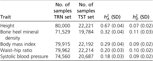
As in Kimet al. (2017), we also analyzed human height because it is a highly heritable trait with a very complex ge-netic architecture and a common human model trait in quan-titative genetic studies (Visscher et al. 2010). However, because human height is known to be a trait with high nar-row-sense heritability, we expect that a large fraction of phe-notypic variance could be captured with a linear model. Therefore, to contemplate traits for which nonadditive effects may be more relevant, we also considered bone heel mineral density (BHMD), body mass index (BMI), systolic blood pres-sure (SBP), and waist–hip ratio (WHR). Not all phenotypes were available for all individuals. The numbers of records available for each trait are given in Table 1. Phenotypes were all precorrected by sex, age, the center where phenotypes were collected, and with the top-10 SNP-derived principal components.

Genotypes

The UK Biobank’s participants were genotyped with a custom Affymetrix Axiom array containing820k (k= 1000) SNPs (http://www.ukbiobank.ac.uk/scientists-3/uk-biobank-ax-iom-array/). Here, SNPfiltering followed the criteria used in Kimet al.(2017). Briefly, SNPs with a minor allele frequency, 0.1% and a missing rate.3% werefiltered out using PLINK 1.9 (Changet al.2015). Mitochondrial and sex chromosome SNPs were also removed, except those in pseudoautosomal regions, yielding a total of 567,867 used SNPs.

For each of the prediction methods described below, we evaluated performance with SNP sets of 10k and 50k SNPs. In set “BEST,”the 10k or 50k top most-associated SNPs, i.e., Table 1 Number of phenotypes available and genetic parameters

Trait No. of samples TRN set No. of samples

TST set h2

A(SD) h2D(SD)

Height 80,000 22,221 0.67 (0.04) 0.07 (0.02) Bone heel mineral

density

71,529 19,784 0.32 (0.04) 0.11 (0.03)

Body mass index 79,915 22,192 0.29 (0.04) 0.09 (0.02) Waist–hip ratio 79,962 22,214 0.20 (0.03) 0.10 (0.02) Systolic blood pressure 74,560 20,687 0.18 (0.03) 0.09 (0.02)

h2A: Posterior density median and SD of genomic heritability.h

2

D:Posterior density median and SD of genomic dominance variance (% of phenotypic variance).h2

(3)

those with the lowestP-values in a GWAS on the TRN set for each trait, were chosen. In set“UNIF,”the genome was split in windows of equal physical length and the most-associated SNP within each window was chosen. This criterion was cho-sen to accommodate the philosophy of CNNs, which are designed to utilize the correlation between physically adja-cent input variables (see below). Windows were 309- and 61-kb long in the 10k and 50k SNP UNIF sets, respectively.

Variance components analyses

We estimated the proportion of variance that could be explained by additive and dominance effects using a genomic best linear unbiased prediction (GBLUP) model (VanRaden 2008). The additive genomic relationship matrix for additive effects was computed as in VanRaden’s equation

G¼ XX’

2Pmj¼1qj ð12qjÞ;

whereXis ann3mmatrix (nindividuals andmmarkers) that contains the centered individual genotype values, i.e., 22qj, 122qj, and 222qjwhen genotypes are coded as 0, 1,

and 2, withqjbeing the allele frequency of alternative allele “1”atj-th SNP. The dominance relationship matrix was cal-culated as proposed in Vitezicaet al.(2013):

D¼ MM’

4Pmj¼1½qj ð12qjÞ2

;

where the elements of matrix Mnxm are 22qj2, 2qj(12qj),

and22(12qj)2for genotypes 0, 1, and 2, respectively. Due

to computational constraints, 10,000 random individuals from the TRN set were used to build the genomic relationship matrices, although with all markers.

Bayesian linear models

BayesB (Meuwissenet al.2001) and Bayesian Ridge Regres-sion (also called BLUP in the animal breeding literature, Henderson 1984) are two widely used genomic linear pre-diction methods; thus, we used these two methods as bench-marks against which we compare DL techniques. In these models, the phenotype of thei-th individual can be expressed as:

yi¼b0þx’ibþei;

where bis a vector with regression coefﬁcients on marker genotypesxiande, a residual term. The likelihood is written as:

pðujyÞ ¼ Y

n

i¼1

N

yi2 b02x’ib;s2e

pðuÞ

The difference between BRR and BayesB lies in the prior speciﬁcationpðuÞ:In BayesB, the parametersuinclude the probabilitypof a given SNP being included in the model, and

this probability in turn is also sampled according to a b bi-nomial distribution, whereas all markers enter into the model for BRR (see,e.g., Pérez and de Los Campos (2014) for fur-ther details).

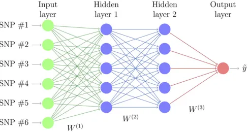
MLPs

MLPs, also called fully connected feed-forward NNs, are commonly used for DL. An MLP consists of at least three layers of nodes (Figure 1). Theﬁrst layer, known as the input layer, consists of a set of neurons (xi,j =1,m) representing the input features (SNP genotypes). Each neuron in the hidden layer transforms the values from the previous layer with a weighted linear summation,i.e., for theﬁrst layer and l-th neuronaðl1Þ¼

Pm

j¼1w

ð1Þ

lj xjþb

ð1Þ

0 ;wherew

ð1Þ

lj is the weight of

l-th neuron toj-th input in theﬁrst layer,b0is the intercept

(called“bias”in machine learning literature), followed by a nonlinear activation function f(al) that results in neuron’s

output. Subsequent layers receive the values from the pre-vious layers and the last hidden layer transforms them into output values. Learning occurs in the MLP by changing weights (w) after each piece of data is processed, such that the loss function is minimized. This process is carried out through back-propagation, a generalization of the least squares algorithm in the linear perceptron (Rosenblatt 1961; Rumelhartet al.1986; LeCunet al.1998a). The multiple layers and nonlinear activation distinguish an MLP from a linear perceptron and make them far more versatile for representing complex outputs. An issue with MLPs is the need to optimize the neuron architecture, which depends on numerous param-eters: activation function, dropout rate (i.e., the rate at which a random neuron is removed from the model, Srivastavaet al. 2014), and the number of layers and neurons per layer. See sectionHyperparameter optimizationbelow.

(4)

taking values 0, 1, and 2 for the three genotypes, as we did for the rest of the MLPs and CNNs described below.

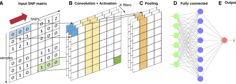
CNNs

CNNs (LeCun and Bengio 1995; LeCun et al.1998b) are a specialized kind of NN for data, where inputs are associated with each other and exploit that fact. The hidden layers of a CNN typically consist of convolutional layers, pooling layers, fully connected layers, and normalization layers. CNNs com-bine several layers of convolutions with nonlinear activation functions. Figure 2 shows a general diagram of a CNN. During the training phase, a CNN automatically learns the coefficients of the so called“filters.”Afilter is defined as a combination of the input values where the weights are the same for all input windows (e.g., SNP windows). For example, in image classification, a CNN may learn to detect edges from raw pixels in thefirst layer, and then use the edges to detect simple shapes (say circles) in the second layer. Then, these shapes can be used by the next layer to detect even more complex features, say facial shapes. Finally, the last layer is then a classifier that uses these high-level features. These learntfilters are then used across all input variables. How-ever, to make them slightly invariant to small translations of the input, a pooling step is added. CNNs have shown great success in computer vision, where pixel intensities of images are locally correlated. In the genomic prediction context, adjacent SNP ge-notypes are expected to be correlated due to linkage disequilib-rium. In this case, it makes sense to use one-dimensional kernels, as opposed to two-dimensional kernels used for images. This means that sliding sets of s consecutive SNPs are used for each filter (Figure 2), instead of squares of pixels.

Hyperparameter optimization

Hyperparameter optimization is a fundamental step for DL implementation since it can critically inﬂuence the predictive

performance of MLPs and CNNs. Here, we applied a modified genetic algorithm as implemented in DeepEvolve (Liphardt 2017) to evolve a population of MLPs or CNNs with the goal of achieving optimized hyperparameters in a faster manner than with traditional grid or random searches. The algorithm is described in Supplemental Material, Figure S1 and the different parameters optimized together with their theoreti-cal effects on the model capacity are presented at Table S1. This optimization was done for each trait independently us-ing the TRN set and the 10k BEST SNP set in two steps. In the first step, we selected the bestfive architectures for each of thefive traits independently. Next, all 25 solutions were eval-uated for the remaining traits. Finally, we selected the best three MLPs and CNNs that performed uniformly best across traits.

Assessment of prediction accuracy

For all prediction methods, parameters were estimated by regressing the adjusted phenotypes on SNPs set using data from the TRN set. Subsequently, we applied thefitted model to genotypes of the TST data set and evaluated prediction accuracy by correlating (R) the SNP-derived predicted phe-notype with the adjusted phephe-notype in the TST set. Since the MLP or CNN depends, to an extent, on initialization values, we ran each case six times and we retained the best learner in the TRN stage,i.e., using only the TRN set. Approximate lower-bound SE’s of R were obtained frompffiffiffiffiffiffiffiffiffiffiffiffiffiffiffiffiffiffiffiffiffiffiffiffiffiffiffiffiffiffiffiffiffiffiffiffið12R2_Þ₌_ð_n₂₂_Þ_;_n

being the TST data size.

Software

(5)

Bayesian GBLUP using BRR prior and eigenvalue decompo-sition ofGandDwas employed to estimate genomic herita-bilities with the BGLR package [see Forneriset al.(2017) for an application of this model]. Genomic matrices were com-puted with a Fortran program that employs Basic Linear Al-gebra Subroutines (BLAS) (Dongarra et al. 1990, www. netlib.org/blas/) for efficient parallelization, available at https://github.com/miguelperezenciso/dogrm. The rest of the analyses were implemented in python using scikit (Pedregosaet al.2011,www.scikit-learn.org), pandas (pan-das.pydata.org), and numpy (www.numpy.org/) among other libraries for the processing and analysis of the data. To implement machine learning methods, we used the Keras API (Chollet 2015, www.keras.io), which provides a high-level NN API on top of Tensorflow (Abadiet al.2015,www. tensorflow.org) libraries. Software and pipelines are avail-able athttps://github.com/paubellot/DL-Biobank.

Data availability

This research has been conducted using the UK Biobank Re-source under project identiﬁcation number 15326. The data are available for allbonaﬁderesearchers and can be acquired by applying athttp://www.ukbiobank.ac.uk/register-apply/. The Institutional Review Board (IRB) of Michigan State Uni-versity has approved this research with the IRB number 15– 745. The three authors completed IRB TRN. Lists of SNPs and P-values are available at https://github.com/paubellot/DL-Biobank. Supplemental material contains a summary of main

DL parameters, a description of the genetic algorithm used for hyperparameter optimization, and additional MLP and CNN results. Supplemental material available at Figshare: https://doi.org/10.6084/m9.ﬁgshare.7035866.

Results

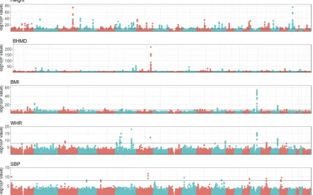
Thefive phenotypes analyzed span a wide range of genetic profiles, as the GWAS in Figure 3 and heritabilities in Table 1 show. Height is a well-studied phenotype in thefield of hu-man quantitative genetics and, in agreement with the litera-ture (e.g., Yanget al.2010), the GWAS does show numerous and highly significant peaks scattered throughout the ge-nome: 946 SNPs had a P-value , 1028, the tentative ge-nome-wide significance level. Height was also the trait with highest genomic heritability:h2

A= 0.67 (Table 1). Genomic

heritabilities were markedly lower for the rest of the pheno-types. As expected, the dominance variance for height was small relative to the additive variance; however, the esti-mates of dominance variance were between one-half and one-third of that of the additive variance for the other four traits.

(6)

significant region in a GWAS on a larger subset of the biobank data set. As for BMI and WHR phenotypes, they shared some peaks but they were more significant for BMI. Perhaps related to this, the genomic heritability of BMI was 50% larger than that of WHR (0.29vs.0.20, respectively, Table 1). The heri-tability of SBP was mildly lower than that of WHR and QTL peaks were concordantly less significant. We only found 15 SNPs with aP-value,1028in SBPvs.56 SNPs in WHR.

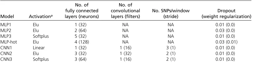
The retained MLPs and CNNs that performed uniformly best across traits are shown in Table 2. MLP1, MLP2, and MLP3 differ mainly in the number of layers: 1, 2, and 5, respectively. For CNNs, the optimum SNP window was very small with maximum overlap (stride = 1), but they differed in activation function, number of neurons, and on number of ﬁlters. For one-hot encoding, we evaluated only one MLP. Overall, the chosen regularization, as inferred from the genetic algorithm, was very small for either MLPs or CNNs (Table 2).

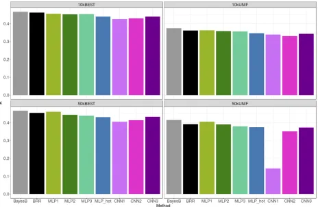
Figure 4 shows the TST correlation (R) between predicted and adjusted height for each of the methods and SNP sets. Overall, all methods performed similarly, although CNN models were slightly worse. Prediction correlations with the linear model were very similar to those reported in Kim et al.(2017), as expected because we used the same data set. Selecting SNPs based only on unrestricted GWAS P-values (BEST set) was systematically better than setting a restriction on the distance between retained SNPs (UNIF set), especially— and paradoxically—for CNNs. Penalized linear methods were not so sensitive to SNP choice, in particular when the total number of SNPs was large (50k). We did not observe a clear improvement in prediction accuracy for any of the methods when increasing the number of SNPs from 10k to 50k. For some CNNs (CNN3), adding SNPs was even detrimental when using the UNIF set.

Figure 5 shows the correlation between predicted and adjusted BHMD in the TST set, which displays a different picture from that obtained with height (Figure 4). For this phenotype, CNNs performed better overall than MLPs, espe-cially for 10k SNP sets. In particular, CNN3 conﬁguration was comparable or slightly better than Bayesian linear methods. Consistent with the height phenotype though, methods per-formed better with the BEST SNP set than with the UNIF set. For some MLPs and CNNs with the 50k sets, we observed

some convergence problems that persisted even after several reinitializations of the algorithm. This is likely due to the exponential increase in parameters to be learnt in nonlinear methods with large SNP data sets and to the reduced pre-dictive ability, compared to height. However, these issues were not observed with linear methods.

For the rest of the phenotypes, predictive accuracies were lower than for height or BHMD (Figure S2). Similar to what we observed for BHMD, in the case of BMI, WHR and SBP Bayesian linear methods, and the CNN3, were consistently the best methods overall. In some instances though, e.g., BMI, one-hot encoding or MLP2 could be preferred. Differences between top methods were never very large. In general, per-formance of MLPs or CNNs was sensitive to the speciﬁed network architecture, and highly dependent on the pheno-type analyzed (Figure 5 and Figure S2). This was not so much the case for Bayesian linear methods, which were far more stable.

CNNs are designed to exploit a spatially local correlation by enforcing a putative connectivity pattern between nearby inputs. This fact motivated the usage of equally spaced SNP sets (UNIF sets). However, simply selecting SNPs on absolute significance (BEST sets) was a better option across all anal-yses. This indicates that systematic controlling for linkage disequilibrium does not necessarily improve, and can even harm, prediction accuracy. Furthermore, CNN hyperpara-meter optimization suggested that maximum overlapping (stride = 1) between very small windows (2–3 SNPs) was the optimum configuration for CNNs (Table 2). To further investigate the effect of SNP spacing and stride on CNNs, we fitted CNN3 for height phenotype varying the overlap (max-imumvs.no overlap) and SNP window size (2–10 SNPs). We observed that overlapping between windows was better than no overlapping, and small windows (2–3 SNPs) should be preferred to large ones when using the BEST criterion (Table S2). In the case of uniformly distributed SNPs, differences between criteria were relatively small.

Discussion

With this work, we aim to stimulate debate and research on the use of DL techniques for genomic prediction. DL is Table 2 Main features of chosen MLPs and CNNs

Model Activationa

No. of fully connected layers (neurons)

No. of convolutional layers (ﬁlters)

No. SNPs/window (stride)

Dropout (weight regularization)

MLP1 Elu 1 (32) NA NA 0.01 (0.0)

MLP2 Elu 2 (64) NA NA 0.03 (0.0)

MLP3 Softplus 5 (32) NA NA 0.01 (0.0)

MLP-hot Elu 4 (128) NA NA 0.03 (0.01)

CNN1 Linear 1 (32) 1 (16) 3 (1) 0.01 (0.0)

CNN2 Elu 3 (32) 1 (32) 2 (1) 0.01 (0.0)

CNN3 Softplus 3 (64) 1 (16) 2 (1) 0.01 (0.0)

No., number; MLP, Multilayer Perceptron; Elu, exponential linear unit; CNN, Convolutional Neural Network.

(7)

prevailing in areas such as computer vision (LeCun et al. 2015), in part due to its ability to extract useful features (i.e., to learn a hierarchical-modular feature space from vi-sual space) and the ability of DL to map from these derived features into outputs (either a quantitative outcome or a set of labels). In these problems, the label is usually perfectly known and the input visual space consists of complex fea-tures, sometimes of mixed types, whose values vary over wide ranges but are locally correlated. The natures of com-plex trait analyses using SNP data are very different. First, the attribute (the expected value of a trait or genetic risk) is not observable. Rather, we observe a noisy version of it, which is a function of both DNA-sequence and environmental factors. Moreover, the inputs used in genomic prediction are much simpler (SNP genotypes can take only three values) and much more structured than the ones used in computer vision or other areas where DL has thrived. Furthermore, since al-lele frequencies of SNP genotypes are highly unbalanced, a large number of SNP genotypes can be considered as simple 0/1 bits. The complex and noisy nature of the phenotypes, and the relatively simple nature of the input data, may ex-plain why DNA-based prediction linear models perform sim-ilarly, and in many cases better, than DL.

The relative performance of DL vs. linear methods depended on the trait analyzed but also on the DL network

architecture. For height, a highly polygenic trait with a pre-dominant additive genetic basis, there were no large differ-ences between methods, although linear methods prevailed. This was not likely due to a limitation in the size of the data but to the nature of the problem, which apparently can be approximated rather well with a linear model. CNNs were the worst-performing method in height, whereas the perfor-mance of the simplest MLP (MLP1) was nearly undistinguish-able from BayesB or BRR (Figure 4). In contrast, some CNNs were comparable or slightly outperformed linear methods for BHMD, WHR, and SBP in some instances (Figure 5 and Fig-ure S2).

(8)

methods). The highly skewed distribution of allele frequen-cies makes it difﬁcult to accurately consider all three geno-type effects. Note also that one-hot encoding results in an increase in the number of parameters, increasing the risk of overﬁtting.

MLPs and CNNs are actually highly heterogeneous clas-ses of predictors. Depending on the configuration (e.g., on the number of layers, number of neurons per layer, or the activation function used, Table S1), very different models can be obtained. In addition to selecting the network con-figuration, hyperparameters that control regularization need to be estimated as well. Finding an optimal configu-ration for an MLP or CNN can be challenging. Here, we used a genetic algorithm to perform this optimization. Ge-netic algorithms are a well-known (e.g., Mitchell 1998) approach for maximizing complex functions in cases such as the one considered here, where optimum hyperpara-meter values are highly dependent between them. The complexity of DL methods contrasts with the frugality of penalized linear regressions, where the search is con-strained to the class of linear models and the only estimation problem consists offinding weights associated with each of the inputs.

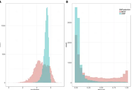
It was computationally impossible toﬁt all500k SNPs with 100k subjects in an MLP or a CNN, and some feature

(9)

proﬁles in Figure 3). In terms of linkage disequilibrium (measured as correlation between genotype values at two SNPs), the differences were dramatic since LD was very low genome-wide (UNIF set), whereas LD was much higher in the BEST sets (Figure 6b). In summary, choosing SNPs based only on individualP-values resulted in groups of clustered SNPs, the structures of which were better exploited by CNNs than when SNPs were chosen at equal intervals. As a result, CNNs performed better than some MLPs for BHMD or other traits (Figure 5 and Figure S2).

Our analyses show that CNNs performed comparatively better as narrow-sense heritability decreased and the con-tribution of dominance increased. Therefore, in our opin-ion, future efforts in DL research for genomic prediction should aim at improving mapping functions to overcome linear constraints that relate genotype to phenotype. For CNNs, methods for optimum exploitation of SNP disequi-librium in CNNs are also needed. A major problem here is that LD varies along the genome and therefore optimum SNP window sizes are not constant. This problem is similar to that found in learning from text, where the length of each document varies. Therefore, each individual word cannot be used as an input feature, because long documents and words would require different input spaces to shorter ones. Researchers in text machine learning have proposed several

methods to address those issues such as classical “bag of words” (BOW, Salton and McGill 1983) or more recent word2vec (Mikolovet al.2013) algorithms. The basic idea of both methods is to represent documents or words with numbers, turning text into a numerical form that DL can understand. BOW is based on the frequency of words, whereas word2vec maps every word into a vector, so sim-ilar words are closer. To use genotypes in CNNs more ef-ﬁciently, a similar approach could be explored. This representation should be smaller and length-independent, and yet able to encode the SNPs’information. To the best of our knowledge, CNNs have not been applied to human genetic prediction so far, but here we show that they are promising tools that deserve future research.

Acknowledgments

This work was funded by project grant AGL2016-78709-R (Ministerio de Economía y Competitividad, Spain) to M.P.-E., and National Institutes of Health grants R01-GM-101219 and R01-GM-099992 (USA) to G.d.l.C. and M.P.-E. The Cen-tre for Research in Agrogenomics receives the support of

“Centro de Excelencia Severo Ochoa 2016–2019” award SEV-2015-0533 (Ministerio de Economía y Competitividad, Spain).

(10)

Literature Cited

Abadi, M., A. Agarwal, P. Barham, E. Brevdo, Z. Chen et al.,

2015 TensorFlow: large-scale machine learning on

heteroge-neous systems. Available at: tensorﬂow.org. Accessed: July 1,

2018.

Alipanahi, B., A. Delong, M. T. Weirauch, and B. J. Frey,

2015 Predicting the sequence speci_ﬁcities of DNA- and

RNA-binding proteins by deep learning. Nat. Biotechnol. 33: 831_–

838.https://doi.org/10.1038/nbt.3300

Chang, C. C., C. C. Chow, L. C. Tellier, S. Vattikuti, S. M. Purcell et al., 2015 Second-generation PLINK: rising to the challenge

of larger and richer datasets. Gigascience 4: 7.https://doi.org/

10.1186/s13742-015-0047-8

Chollet, F., 2015 Keras: deep learning library for theano and

ten-sorﬂow. Available at:https://keras.io/. Accessed May 1, 2018.

de Los Campos, G., and A. Grueneberg, 2017 BGData: a suite

of packages for analysis of big genomic data. R package

ver-sion 1.0.0.9000. Available at:https://github.com/QuantGen/

BGData

de los Campos, G., D. Gianola, and D. B. Allison, 2010 Predicting

genetic predisposition in humans: the promise of whole-genome

markers. Nat. Rev. Genet. 11: 880–886.https://doi.org/10.1038/

nrg2898

de los Campos, G., J. M. Hickey, R. Pong-Wong, H. D. Daetwyler,

and M. P. Calus, 2013 Whole-genome regression and

pre-diction methods applied to plant and animal breeding.

Ge-netics 193: 327_–345.https://doi.org/10.1534/genetics.112.

143313

Dongarra, J. J., J. Du Croz, S. Hammarling, and I. S. Duff, 1990 A

set of level 3 basic linear algebra subprograms. ACM Trans.

Math. Softw. 16: 1–17.https://doi.org/10.1145/77626.79170

Forneris, N. S., Z. G. Vitezica, A. Legarra, and M. Pérez-Enciso,

2017 Inﬂuence of epistasis on response to genomic selection

using complete sequence data. Genet. Sel. Evol. 49: 66.https://

doi.org/10.1186/s12711-017-0340-3

Gianola, D., H. Okut, K. A. Weigel, and G. J. Rosa, 2011 Predicting

complex quantitative traits with Bayesian neural networks: a case

study with Jersey cows and wheat. BMC Genet. 12: 87.https://

doi.org/10.1186/1471-2156-12-87

González-Camacho, J. M., G. de Los Campos, P. Pérez, D. Gianola,

J. E. Cairnset al., 2012 Genome-enabled prediction of genetic

values using radial basis function neural networks. Theor. Appl.

Genet. 125: 759_–771.

https://doi.org/10.1007/s00122-012-1868-9

González-Camacho, J. M., J. Crossa, P. Pérez-Rodríguez, L. Ornella,

and D. Gianola, 2016 Genome-enabled prediction using

prob-abilistic neural network classi_ﬁers. BMC Genomics 17: 208.

https://doi.org/10.1186/s12864-016-2553-1

Goodfellow, I., Y. Bengio, and A. Courville, 2016 Deep Learning.

MIT Press, Cambridge, MA.

Henderson, C. R., 1984 Applications of Linear Models in Animal

Breeding. University of Guelph, Guelph, ON.

Kelley, D. R., J. Snoek, and J. L. Rinn, 2016 Basset: learning the

regulatory code of the accessible genome with deep

convolu-tional neural networks. Genome Res. 26: 990–999.https://doi.

org/10.1101/gr.200535.115

Kemp, J. P., J. A. Morris, C. Medina-Gomez, V. Forgetta, N. M.

Warringtonet al., 2017 Identiﬁcation of 153 new loci

associ-ated with heel bone mineral density and functional involvement

of GPC6 in osteoporosis. Nat. Genet. 49: 1468_–1475.https://

doi.org/10.1038/ng.3949

Kim, H., A. Grueneberg, A. I. Vazquez, S. Hsu, and G. de Los Campos,

2017 Will big data close the missing heritability gap?

Genetics 207: 1135_–1145.https://doi.org/10.1534/genetics.117.

300271

LeCun, Y., and Y. Bengio, 1995 Convolutional Networks for

Im-ages,Speech,and Time Series. MIT Press, Cambridge, MA.

LeCun, Y., L. Bottou, G. B. Orr, and K. R. Muller, 1998a Efﬁcient

BackProp, pp. 9–50 in Neural Networks: Tricks of the Trade,

edited by G. B. Orr and K. R. Müller. Springer-Verlag, Berlin.

10.1007/3-540-49430-8_2.

https://doi.org/10.1007/3-540-49430-8_2

LeCun, Y., L. Bottou, Y. Bengio, and P. Haffner, 1998b

Gradient-based learning applied to document recognition. Proc. IEEE 86:

2278–2324.https://doi.org/10.1109/5.726791

LeCun, Y., Y. Bengio, and G. Hinton, 2015 Deep learning. Nature

521: 436–444.https://doi.org/10.1038/nature14539

Lee, S. H., N. R. Wray, M. E. Goddard, and P. M. Visscher,

2011 Estimating missing heritability for disease from

genome-wide association studies. Am. J. Hum. Genet. 88: 294–305.

https://doi.org/10.1016/j.ajhg.2011.02.002

Liphardt, J., 2017 DeepEvolve: rapid hyperparameter discovery

for neural nets using genetic algorithms. Available at:https://

github.com/jliphard/DeepEvolve/. Accessed: January 2018.

Maher, B., 2008 Personal genomes: the case of the missing

heri-tability. Nature 456: 18–21.https://doi.org/10.1038/456018a

Meuwissen, T. H. E., B. J. Hayes, and M. E. Goddard,

2001 Prediction of total genetic value using genome-wide

dense marker maps. Genetics 157: 1819–1829.

Meuwissen, T. H. E., B. Hayes, and M. Goddard, 2013 Accelerating

improvement of livestock with genomic selection. Annu. Rev.

Anim. Biosci. 1: 221–237.

https://doi.org/10.1146/annurev-animal-031412-103705

Mikolov, T., K. Chen, G. Corrado, and J. Dean, 2013 Efﬁcient

estimation of word representations in vector space. arXiv: 1301.3781v3 [cs.CL].

Mitchell, M., 1998 An Introduction to Genetic Algorithms. MIT

Press, Cambridge, MA.

Nguyen, T. V., G. Livshits, J. R. Center, K. Yakovenko, and J. A.

Eisman, 2003 Genetic determination of bone mineral density:

evidence for a major gene. J. Clin. Endocrinol. Metab. 88: 3614_–

3620.https://doi.org/10.1210/jc.2002-030026

Okut, H., D. Gianola, G. J. Rosa, and K. A. Weigel, 2011 Prediction

of body mass index in mice using dense molecular markers and a

regularized neural network. Genet. Res. (Camb) 93: 189–201.

https://doi.org/10.1017/S0016672310000662

Pedregosa, F., G. Varoquaux, A. Gramfort, V. Michel, B. Thirion et al., 2011 Scikit-learn: machine learning in Python. J. Mach.

Learn. Res. 12: 2825–2830.

Pérez, P., and G. de Los Campos, 2014 Genome-wide regression &

prediction with the BGLR statistical package. Genetics 198: 483–495.https://doi.org/10.1534/genetics.114.164442

Pérez-Rodríguez, P., D. Gianola, J. M. González-Camacho, J.

Crossa, Y. Manès et al., 2012 Comparison between linear

and non-parametric regression models for genome-enabled

pre-diction in wheat. G3 (Bethesda) 2: 1595–1605.https://doi.org/

10.1534/g3.112.003665

Rosenblatt, F., 1961 Principles of neurodynamics. Perceptrons and

the theory of brain mechanisms. Spartan Books, Washington, DC.

Rumelhart, D. E., G. E. Hinton, and R. J. Williams, 1986 Learning

representations by back-propagating errors. Nature 323: 533–

536.https://doi.org/10.1038/323533a0

Salton, G., and M. McGill, 1983 Introduction to Modern

Informa-tion Retrieval. McGraw-Hill, New York.

Srivastava, N., G. Hinton, A. Krizhevsky, I. Sutskever, and R. Salakhutdinov,

2014 Dropout: a simple way to prevent neural networks from

overﬁtting. J. Mach. Learn. Res. 15: 1929–1958.

Stranger, B. E., E. A. Stahl, and T. Raj, 2011 Progress and promise

of genome-wide association studies for human complex trait

genetics. Genetics 187: 367–383. https://doi.org/10.1534/

(11)

VanRaden, P. M., 2008 Efﬁcient methods to compute genomic

predictions. J. Dairy Sci. 91: 4414–4423. https://doi.org/10.

3168/jds.2007-0980

Visscher, P. M., B. McEvoy, and J. Yang, 2010 From Galton to

GWAS: quantitative genetics of human height. Genet. Res. 92: 371–379.https://doi.org/10.1017/S0016672310000571

Vitezica, Z. G., L. Varona, and A. Legarra, 2013 On the additive

and dominant variance and covariance of individuals within the

genomic selection scope. Genetics 195: 1223–1230.https://doi.

org/10.1534/genetics.113.155176

Wan, X., C. Yang, Q. Yang, H. Xue, X. Fanet al., 2010 BOOST: a

fast approach to detecting gene-gene interactions in genome-wide

case-control studies. Am. J. Hum. Genet. 87: 325–340.https://

doi.org/10.1016/j.ajhg.2010.07.021

Yang, J., B. Benyamin, B. P. McEvoy, S. Gordon, A. K. Henderset al.,

2010 Common SNPs explain a large proportion of the

herita-bility for human height. Nat. Genet. 42: 565–569.https://doi.

org/10.1038/ng.608

Zhou, J., and O. G. Troyanskaya, 2015 Predicting effects of

non-coding variants with deep learning-based sequence model.

Nat. Methods 12: 931–934. https://doi.org/10.1038/nmeth.

3547