Fixation Probability in a Haploid-Diploid Population
Kazuhiro Bessho*,1and Sarah P. Otto†,1 *JSPS Research Fellow, Department of Evolutionary Studies of Biosystems, School of Advanced Sciences, SOKENDAI (The Graduate University for Advanced Studies), Hayama, 240-0193, Japan, and†Department of Zoology, University of British Columbia, Vancouver, V6T 1Z4, Canada ORCID ID: 0000-0003-3042-0818 (S.P.O.)
ABSTRACT Classical population genetic theory generally assumes either a fully haploid or fully diploid life cycle. However, many organisms exhibit more complex life cycles, with both free-living haploid and diploid stages. Here we ask what the probability of fixation is for selected alleles in organisms with haploid-diploid life cycles. We develop a genetic model that considers the population dynamics using both the Moran model and Wright–Fisher model. Applying a branching process approximation, we obtain an accurate fixation probability assuming that the population is large and the net effect of the mutation is beneficial. We alsofind the diffusion approximation for thefixation probability, which is accurate even in small populations and for deleterious alleles, as long as selection is weak. These fixation probabilities from branching process and diffusion approximations are similar when selection is weak for beneficial mutations that are not fully recessive. In many cases, particularly when one phase predominates, thefixation probability differs substantially for haploid-diploid organisms compared to either fully haploid or diploid species.
KEYWORDSfixation probability; Moran model; Wright–Fisher model; haploid-diploid life cycle; variance effective population size
C
LASSICAL genetic theories generally assume either a fully haploid (haplont) or fully diploid (diplont) life cycle (e.g., Crow and Kimura 1970). Organisms often exhibit more com-plex sexual life cycles, however, with both free-living haploid and diploid stages (haploid-diploid life cycle) (Mable and Otto 1998). For example, marine macroalgae generally exhibit an alternation of generations between a haploid-gametophyte stage and a diploid-sporophyte stage (Bell 1994, 1997). Furthermore, haploid and diploid life stages can differ substantially in morphology. For example, diploid-dominant species (e.g., Laminariales) have large diploid spo-rophytes and small haploid gametophytes, with the reverse found in haploid-dominant species (e.g.,Cutleriales multifida) (Hirose 1975; Bell 1994, 1997).Despite haploid-diploid life cycles being common in several groups of organisms, classical population genetic quantities,
such as thefixation probability and the effective population size, have not been determined for haploid-diploid organ-isms. Thefixation probability is fundamental to predicting the rate of adaptation of a species with an alternation be-tween free-living haploid and diploid generations. It is also important for predicting the ability of organisms to persist in a changing environment and to predict how patterns of molecular evolution depend on the life cycle. Indeed, a total of 5480 articles mention the probability of fixation in a genetic context [Google Scholar search, September 10, 2016: (“fixation probability” k “probability of fixation”) (genekgenetickallelekmutationkmutant)], in contexts rang-ing from the interpretation of sequence data, to the predic-tion of quantitative trait variapredic-tion, to the spread of disease resistance,etc.
In addition, thefixation probability is needed to model the evolution of the life cycle itself (i.e., the relative pro-portion of haploidy vs.diploidy), when one accounts for several of the complexities seen in haploid-diploid species such as coexistence of haploids and diploids in a popula-tion (e.g., Destombe et al. 1989; Hiraoka and Yoshida 2010) and differences in spatial distribution and dispersal ability (e.g., Bell 1997). In a related article, we model the dynamics of a modifier allele controlling the life cycle (Mable and Otto 1998), explicitly tracking the demographic Copyright © 2017 by the Genetics Society of America
doi: 10.1534/genetics.116.192856
Manuscript received July 6, 2016; accepted for publication November 10, 2016; published Early Online November 17, 2016.
Supplemental material is available online athttp://doi.org/10.5061/dryad.n4k76.
1Corresponding authors: Department of Evolutionary Studies of Biosystems, School of
Advanced Sciences, SOKENDAI (The Graduate University for Advanced Studies), Shonan Village, Hayama, Kanagawa 240-0193, Japan. E-mail: bessho_kazuhiro@ soken.ac.jp; and Department of Zoology, 6270 University Blvd., University of British Columbia, Vancouver, BC, V6T 1Z4, Canada. E-mail: [email protected]
and S. P. Otto, unpublished data). This related work re-quires the fixation probability in haploid-diploid species, as derived in the current article.
Given the fundamental importance of thefixation prob-ability in evolutionary theory, there is a surprising lack of stochastic analyses describing the fate of selected alleles with haploid-diploid life cycles, compared to the many analyses on exclusively haploid or diploid life cycles (e.g., Crow and Kimura 1970; Ewens 2004). To fill this gap, we develop genetic models that consider the population dynamics for haploid and diploid generations, deriving thefixation probability for a selected allele in such species. These results are further evaluated by comparison to nu-merical simulations.
Model
To calculate thefixation probability, wefirst extended the classical population genetic models, the Moran model and the Wright–Fisher (WF) model, to account for free-living haploid and diploid phases. In these models, we track the haploid and diploid population dynamics and changes in allele frequencies under the assumption of a one-locus ge-netic model with two alleles (resident alleleRand mutant alleleM). We assume the following: (1) that the total pop-ulation sizeNisfixed, (2) that there is an obligate alter-nation of generations between haploid and diploid phases, (3) that the species is monoecious with equal invest-ment in male and female gametes, and (4) that mating is random.
Because the number of individuals with genotype (GT) is a Markov process over time in both Moran and WF models, we letXðGTÞðtÞrepresent the number at timetas a random variable, and we letxðGTÞrepresent the realized number in a given generation. The index (GT) indicates the genotype of individuals or cells [(GT) = R or M for haploids and (GT) = RR, RM, or MM for diploids]. Summed over all genotypes, the population size is NðxRþxMþxRRþxRMþxMM¼NÞ. Parameters and
vari-ables in our model are represented in Table 1.
Moran model
In the Moran model, at every time step, death, reproduction, fertilization, and recruitment occur. First, one individual is randomly eliminated from the population in proportion to its mortality rate dðGTÞ: This individual is then replaced by a birth. At reproduction, diploids produce haploid spores at rate bðGTÞ ½0,bðGTÞ;and haploids produce female haploid gametes at ratebðGTÞ=2 [and male gametes at ratebðGTÞ=2: The female gametes can be fertilized with male gametes with a fertilization success offðGTÞ½0,fðGTÞ,1;where we assume that male gametes are not limiting. All haploid spores and fertilized diploid zygotes are candidate reproductive cells to replace the dead individual and are equally likely to be recruited.
We next consider a different type of population dynamics using the WF model. In this model, all diploids produce a numberwðGTÞ½0,wðGTÞof spores, and haploids produce wðGTÞ=2 female gametes ½andwðGTÞ=2 male gametes: As before, the female gametes are fertilized with male gametes with a fertilization success rate offðGTÞ½0,fðGTÞ,1:After the end of each time step, all parents are eliminated from the population, and the next generation is constructed by randomly sampling N individuals in proportion to the number of haploid spores and diploid zygotes produced by the previous generation (see Equation D1).
Individual-based simulations
To check the accuracy of the analytical results, we simu-lated the dynamics numerically. We started the system
fixed on the R allele, assuming that the system has reached ecological and demographic equilibrium (i.e., in the ab-sence of selection, see Appendix A and Appendix D for details), withH^¼^rModelH Nhaploids andD^¼^rModelD N dip-loids (rounded to have integer numbers of individuals) and with^rModelH ¼12^rModelD giving the frequency of hap-loids in the population (see Equation A8b for the Moran model and Equation D2 for the WF model). Next, we mutated one resident allele at random and simulated until this allele was fixed or lost in the population. To estimate thefixation probability, we repeated the process and estimated the probability from the resulting fre-quency offixation.
Data availability
The analysis, numerical simulations, and scripts to gen-erate the originalfigures were coded in Wolfram Math-ematica 10 (Supplemental Material, File S1), available for download from the Dryad Digital Repository (http:// doi.org/10.5061/dryad.n4k76).
Results
Fixation probability
Fixation probabilities in the Moran model using a
branching process approximation: We first develop a
branching process approximation (e.g., Haldane 1927; Yeaman and Otto 2011) for haploid-diploid life cycle spe-cies. Specifically, we calculate the fixation probability of a single allele that appears in the haploid phase (geno-typeM),pMoranH ;and thefixation probability for a single
allele that appears in a heterozygous diploid (genotype RM),pMoranD ;after which we calculate the average
proba-bility offixation for an allele that appears randomly in any individual. When using a branching process approach, the fates of mutations in different individuals are assumed to be independent of one another, which implicitly requires that the population size is large and that mutant alleles are lost or established while rare. Under these assumptions,
we obtain approximations for the fixation probabilities (Appendix B):
pMoranH ¼ f~MfRM2f~RfRR ~
fMfRMþfRM2
ffiffiffiffiffiffiffiffiffiffiffiffiffiffi
~ fRfRR
q ; (1a)
pMoranD ¼ f~MfRM2f~RfRR ~
fMfRMþ2f~M
ffiffiffiffiffiffiffiffiffiffiffiffiffiffi
~ fRfRR
q ; (1b)
where we define the expected reproductive rate
fðGTÞ¼bðGTÞ=dðGTÞ;the average fertilization rate for mutant gametesf¼ ðfRþfMÞ=2 (averaged over cases where the
mu-tant is carried by the sperm and when it is carried by the egg), the expected reproductive rate of a haploid mutant
~
fM¼ffM=2;and the expected reproductive rate of a haploid
residentf~R¼fRfR=2:Observe that the expected reproductive
rate of haploids is scaled by the average value offðGTÞfor the combining gametes divided by two, which accounts for the costs of sex (specifically for the possibility that not all female gametes are fertilized and for the fact that haploids must invest half of their reproductive resources in male gametes, which are unable to reproduce on their own). Equations 1a and 1b apply as long as the fixation probabilitiespH andpDare positive,
which occurs when the average mutant fitness is greater than the resident, where the relevant average across the
Symbol Interpretation
pModelH ;ðpModelD Þ Fixation probability in the branching process approximation when the single mutant arises in haploids (diploids); (1) for the Moran model and (D4) for the WF model
uModel
branch Averagefixation probability from the branching process approximation; (2) for the Moran model and (5a) for the WF model
uModel
diffusion Fixation probability from the diffusion approximation; (4) with (3) for the Moran model and (7) for the WF model
p0 Initial allele frequency;p0¼1= N
n
^
rModelH þ2^rModelD
o
N Total population size ^
H;ðD^Þ Number of haploids (diploids) at the population equilibrium;H^¼^rModel
H NandD^¼^rModelD N
^
rModelH ;ð^rModelD Þ Equilibrium fraction of haploids (diploids) in the resident population; (A8) for the Moran model and (D2) for the WF model
d(GT) Mortality rate of an individual with genotype (GT) in the Moran model l(GT) Expected life span of an individual in the Moran model;l(GT)= 1/d(GT) b(GT) Fertility rate of an individual with genotype (GT) in the Moran model w(GT) Fitness of an individual with genotype (GT) in the WF model f(GT) Fertilization success rate of an individual with genotype (GT)
d Arithmetic mean mortality rate;d¼ ðdRþdRRÞ=2
̑
d Harmonic mean mortality rate;d̑¼2=1 dRþ
1 dRR
^
d Weighted mean mortality rate;^d¼dR^rHþdRRr^D
^
b;ðw^Þ Weighted mean fertility rate in the Moran model,fRbR 2^r
Moran
H þbRRr^MoranD
^
w¼fRwR 2 ^r
WF
H þwRR^rWFD in the WF model
f Average fertilization success rate for rare mutant gametes;f¼ ðfRþfMÞ=2
f(GT) Expected reproductive rate of an individual with genotype (GT);fðGTÞ¼bðGTÞ=dðGTÞ ~
fðGTÞ Expected reproductive rate of a haploid individual with genotype (GT) considering the cost of sex;f~M¼ffM=2 andf~R¼fRfR=2
su
ðGTÞ Selection coefficient of the parametersu2 ff;b;d;wg
hu Dominance coefficient of the parametersu2 ff;b;d;wg sModel
ave Average selection coefficient;sMoranave ¼12
sf M 2þs
b
MþsdM
þ1 2ðs
b
RMþsdRMÞfor the Moran model, andsWF
ave¼12
sf M 2þswM
þ1
2swRMfor the WF model
NModel
e Effective population size relative to the diploid-only WF model; (8)
sModel
e Effective selection coefficient; (9a) for the Moran model and (10a) for the WF model
hModel
e Effective dominance coefficient; (9b) for the Moran model and (10b) for the WF model
x(GT) Number of individual with genotype (GT)
c(GT) Number of haploid spores (A2) and diploid zygotes (A3) with genotype (GT) ~
dðGTÞ Probability that an individual with genotype (GT) is eliminated from the population; (A1)
q(GT) Probability that genotype (GT) is recruited into the empty site; (A4)
mModel, (vModel) First (second) moment of change in allele frequency; (3) for the Moran model and (7) for the WF model X(GT)(t) Random variable describing the number of individual with genotype (GT) at timet
pM Average allele frequency weighted appropriately so that the dynamics of weak selection depend only on the allele frequency;pM¼lRþlRlRRpHþ
lRR
lRþlRRpDfor the Moran model, andpM¼ 1 2pHþ
1
2pDfor the WF model
pH, (pD) Allele frequency in haploids (diploids);pH¼xRxþMxMandpD¼
ðxRM=2ÞþxMM xRRþxRMþxMM
dp Difference in allele frequencies between haploids and diploids;dp¼pD2pH
rH Frequency of haploids in the entire population;rH¼ ðxRþxMÞ=N
FD Departure from Hardy–Weinberg in diploids;FD¼122pDð112pDÞxRRþxxRMþRMxMM
condition agrees with the invasion condition in a determin-istic model (K. Bessho and S. P. Otto, unpublished data). When haploids and diploids have similar reproductive rates
ðf~M fRMÞ;thefixation probability of a mutation appearing first in a haploid tends to be larger than a mutation appearing
first in a diploidðpMoran
H .pMoranD Þ;because all of the haploid
mutant offspring bear the mutant allele, whereas only half of the offspring of anRMdiploid do. As the cost of sex rises, however
ðf~Mdeclines relative tofRMÞ;the probability offixation becomes
increasingly more likely when the mutantfirst appears in a dip-loid, thereby delaying this cost.
The average fixation probability of a new mutation that arises uniformly at random among the individuals present in the resident population,uMoran
branch;can then be defined as:
uMoranbranch¼ ^r Moran
H ^
rMoranH þ2^rMoranD p
Moran
H þ
2^rMoranD ^
rMoranH þ2^rMoranD p
Moran
D ;
(2)
where ^rMoranH ¼
ffiffiffiffiffiffiffiffiffiffiffi
bRRdRR
p
ffiffiffiffiffiffiffiffiffiffiffiffiffiffi fRbRdR=2
p
þ ffiffiffiffiffiffiffiffiffiffiffibRRdRR
p is the equilibrium
propor-tion of haploids in the resident populapropor-tion (A8b) and where the“2”accounts for the fact that diploids carry two alleles that could have potentially mutated. Equation 2 allows the
fixation probability to be calculated for arbitrarily strong se-lection, but it will be accurate only as long as the fixation probabilities (1) are not negative.
Fixation probabilities in the Moran model using a diffusion approximation:Next, we derive thefixation prob-ability of a selected mutant allele in a haploid-diploid pop-ulation using Kolmogorov’s backward equation, given the
first and second moments for thefluctuations in allele fre-quencies. This diffusion equation provides an adequate approximation for the fixation probability even for small populations and deleterious mutations (e.g., Kimura 1957), unlike a branching process approximation. Rather than ana-lyzing the genotype frequencies, x(GT), we transform the
model into a new set of variables that allow us to perform a separation of timescales, assuming that selection occurs on a slower timescale and that ecological and demographic processes rapidly bring the system to a“quasi-equilibrium” (see Appendix C). This approach allows the dynamics of the mutant allele to be described by moments that depend only on the parameters and the current allele frequency (Appendix C). Specifically, we let the allele frequencies in haploids and diploids equal pH¼xM=ðxRþxMÞ and pD¼ ðxRM=2þ
xMMÞ=ðxRRþxRMþxMMÞ;respectively, and focus on the
fol-lowing new variables: the difference in allele frequencies between haploids and diploids dp¼pD2pH;the frequency
of haploids in the populationrH ¼ ðxRþxMÞ=N;the
depar-ture from the Hardy–Weinberg principle in diploids FD¼122p 1
Dð12pDÞ
xRM
xRRþxRMþxMM;and the allele frequency av-eraged across ploidy levels and weighted by the expected
pM¼lRþlRlRRpHþ
lRR
lRþlRRpD:Only with this weighted allele fre-quency is it possible to separate the timescales so that the leading-order change inpMis independent of the other
var-iables (Appendix C). This averaging also corresponds to weighting by the reproductive value of each class (Taylor 1990).
To perform the separation of timescales, we assume selection is weak byfirst defining the following selection [s(GT)] and
dom-inance (h) coefficients: fM¼fRð1þsfMÞ; bM¼bRð1þs b MÞ; bRM¼bRRð1þs
b
RMÞ; bMM¼bRRð1þs b
MMÞ; dM¼dRð12sdMÞ;
dRM¼dRRð12sdRMÞ;dMM ¼dRRð12sdMMÞ;hb¼s b RM=s
b MM;and
hd¼sd
RM=sdMM: We then assume weak selection by setting
su
ðGTÞ¼e~suðGTÞ ðu2 ff;b;dgÞ for each life history parameter, whereeis a small term.
The fast-scale dynamics can be tracked by determining changes in the system to leading orderðe0Þ;assuming that selection alters these dynamics only over a longer period of time. Doing so, wefind that the system rapidly approaches a quasi-equilibrium state where there is a similar allele frequency in haploid and diploid populations ðdp0Þ; the fraction of
haploids is approximatelyrH^rMoranH ;the population is nearly
at Hardy–WeinbergðFD0Þ;and the allele frequency does not
change ðDpM 0Þ (see Appendix C and File S1). We then
calculate the average change in allele frequency to leading order, which requires that we keep linear-order terms in e and which accounts for selection (Appendix C andFile S1).
Furthermore to leading order, the second and higher moments of the change in allele frequency are the same as for the neutral case (i.e., when R and M are equivalent, dropping all terms in-volvingeÞ:Consequently, we derive the second moment for the change in allele frequency using the diffusion limit ðN/NÞ when selection is absent (Appendix C andFile S1), which allows us to determine the variance effective population size for this model. We also confirmed that the third moment goes to zero in the diffusion limit for the Moran model, justifying the use of a diffusion approximation (Karlin and Taylor 1981, p. 165).
Using thefirst and second moments for the expected change in the frequency of mutant alleles,mMoran andvMoran;we can calculate the backward equation for the fixation probability with an initial allele frequencyp0,uMorandiffusionðp0Þ(Appendix C):
vMoranðp0Þd 2uMoran
diffusion dp20 þm
Moranðp0ÞduMorandiffusion
dp0 ¼0; (3a)
where
mMoranðpMÞ ¼NpMð12pMÞ
n
2sMoran ave þpM
h
122hbsb
MMþ
122hdsd MM
io
2 ;
(3b)
vMoranðpMÞ ¼
pMð12pMÞ
h
ðdR=dÞ^rMoranH þ2ðdRR=dÞ^rMoranD
i
4r^MoranH ^rMoranD ;
(3c)
andsave ¼2 2MþsMþsM þ2ðsRMþsRMÞis the average
selection experienced by a rare allele across haploid and diploid stages. Here, we scale time as described in Appen-dix C and define the arithmetic mean mortality rate as
d¼ ðdRþdRRÞ=2:Under the diffusion approximation,
selec-tion is assumed to be weak and of orderOð1=NÞ;in which case both mMoran and vMoran are ofOð1Þ when we take the diffusion limit ðN/NÞ: Solving Equations 3a–3c with the boundary conditions, uModel
diffusionð0Þ ¼0 and uModeldiffusionð1Þ ¼1; we then obtain the fixation probability for any diffusion process (Crow and Kimura 1970, p. 424):
uModeldiffusionðp0Þ ¼ Rp0
0 exp
22Qp9 dp9 R1
0exp½22Qðp9Þdp9
; (4a)
withQðpÞ ¼RmvModelModelððppÞÞdp:When a mutation arises at random on a single chromosome within the population, the expected initial allele frequency is:
p0¼ lR lRþlRR
1
^
H
^ rMoranH ^
rMoranH þ2^rMoranD
þ lRR
lRþlRR
1 2D^
2r^MoranD ^
rMoranH þ2^rMoranD
¼ 1
N^rMoranH þ2^rMoranD ; (4b)
again weighting the allele frequency in each ploidy phase by its longevity.
Fixation probabilities in the WF model using a branching process approximation:We next develop thefixation proba-bilitiesuWF
branchandu WF
diffusionusing the WF model, again applying both branching process and diffusion methods (Appendix D).
The branching process approximation yields a pair of coupled nonlinear equations in pWFH and pWFD (Equations
D4a and D4b), which can be solved numerically to obtain thefixation probabilities for an allele appearing at random within the population when selection is strong:
uWFbranch¼
^ rWFH ^
rWFH þ2r^WFD p
WF
H þ
2^rWFD ^
rWFH þ2^rWFD p
WF
D ; (5a)
where now the fraction of haploids in the resident population is given by^rWFH ¼
ffiffiffiffiffiffi wRR p ffiffiffiffiffi~ wR p
þpffiffiffiffiffiffiwRR (see Equation D2). For compact-ness, we have written thefitness of a resident haploid con-sidering the cost of fertilization and sex asw~R¼fRwR=2:
We can also approximate the fixation probabilitiespWFH
and pWFD explicitly when selection is weak. To do so,
we define wM¼wRð1þswMÞ; wRM¼wRRð1þswRMÞ; wMM¼
wRRð1þswMMÞ; and hw¼swRM=swMM;where again we assume
weak selection by settingsw
ðGTÞ¼e~swðGTÞfor smalle:To leading
order ine;thefixation probabilities for an allele initially in a haploid individual or in a diploid individual become:
pWFH 2w~RwRR
~
wRwRRþw2RR
ffiffiffiffiffiffiffiffiffiffiffiffiffiffi
~
wRwRR p 2sWFave¼
4^rD ^
rWFH þ2^rWFD 2s
WF
ave;
(5b)
pWFD 2w~RwRR
~
wRwRRþ2w~R
ffiffiffiffiffiffiffiffiffiffiffiffiffiffi
~
wRwRR
p 2sWFave¼ 2^r WF
H ^
rWFH þ2^rWFD 2s
WF ave;
(5c)
where the average selective effect for a rare allele in the
WF model is defined assWF ave¼12
sfM
2 þs
w M þ1 2s w
RM:Plugging
Equation 5b and (5c) into (5a), we have
uWFbranch 8^r WF
H ^rWFD
^
rWFH þ2^rWFD
22s WF
ave: (6)
This branching process approximation is valid only for muta-tions whose average effect is beneficialðsWF
ave.0Þ:
Fixation probabilities in the WF model using a diffusion approximation:We also derive thefixation probability using a diffusion approach,uWF
diffusion;finding the appropriate drift and diffusion coefficients for use in Equation 4a. Again, we sought a transformation of variables that allowed a separa-tion of timescales, such that the leading-order term in selec-tion depended only on the parameters and the allele frequency. For the WF model, where all parents die each generation, the appropriate definition of the average mutant allele frequency ispM ¼ ðpHþpDÞ=2 (Appendix D). Applying
the separation of timescales, we obtain the drift and diffusion coefficients:
mWFðpMÞ ¼
NpMð12pMÞ
2sWF
aveþpMð122hwÞswMM
2 ; (7a)
vWFðpMÞ ¼
pMð12pMÞ
^
rWFH þ2^rWFD
8r^WFH ^rWFD ; (7b)
where time is measured in units of N generations (see Appendix D for the derivation). Equation 4a then gives the fixation probability, with the initial allele frequency p0¼1=½NðrWFH þ2rWFD Þ for a mutation appearing at
ran-dom on a single chromosome within the population. In contrast to the branching process approximation, thisfi x-ation probability can be calculated for both beneficial
ðsWF
ave.0Þand deleteriousðsWFave,0Þmutations, but assumes that this selection is weak.
Effective genetic parameters: To compare the fixation probabilities derived above to classical results for fully haploid or fully diploid populations, we define the vari-ance effective population size ðNModel
e Þ; selection coeffi -cient ðsModel
e Þ; and dominance coefficient ðhModele Þ that would give the same fixation probability obtained by a
diffusion approximation in the diploid WF model, a classi-cal standard for comparison.
Wefirst define the variance effective population size using the number of diploid individuals in a WF model that would exhibit the same allele frequency variation for a haploid-diploid species by definingNModel
e =N¼pMð12pMÞ=ð2vModelp Þ
(Ewens 2004). Note thatNewould be the census sizeNin the diploid-only WF model butN/2 in the haploid-only WF model, because we use the diploid WF model to define the effective parameters. From the diffusion approximations above, wefind:
NMorane ¼
2^rMoranH ^rMoranD
ðdR=dÞ^rMoranH þ2ðdRR=dÞ^rMoranD
N; (8a)
NeWF¼ 4^r WF
H r^WFD ^
rWFH þ2^rWFD N: (8b)
Note that the variance effective population size is substantially reduced in populations where one of the phases is rare ð^rModelH 0 or r^ModelD 0Þ; reflecting the increased amount of drift that occurs in that phase in species with a strict alternation of generations. When the death rates are equal ðdR¼dRR¼dÞ; NMorane is half NWF
e ;reflecting the higher variance in reproductive success
that is typically observed in the Moran model com-pared to the WF model (e.g., Otto and Day 2007, p. 583 and p. 643).
We next consider the effective selection and dominance coefficients. To do so, we defineseand heas the selection coefficient and the degree of dominance in the classic dip-loid WF model, in which the drift term for the change in allele frequency is DpM¼sepMð12pMÞ½heþ ð122heÞpM
(see Crow and Kimura 1970). Note that the drift term obtained for haploid-diploid populations per generation
ðmModel=NÞhas the same functional form with respect top
M
(see Equation 3b and Equation 7a). Consequently, we can
findseandhefrom the pair of equations describing the changes in allele frequency whenpM= 0ðDpM=½pMð12pMÞ ¼seheÞ and when pM = 1 ðDpM=½pMð12pMÞ ¼seð12heÞÞ; obtaining:
sMorane ¼2sMoranave þ h
122hb
sbMMþ
122hdsd MM
i
2 ; (9a)
hMorane ¼ 2s Moran ave
4sMoran ave þ
h
122hbsb
MMþ
122hdsd MM
i; (9b)
for the Moran model, and
fi fi
on a linear scale whensModel
ave $0:Curves give the branching process results allowing for strong selection [red; Moran from (2) with (1); WF from (5a) with (D4)], the weak-selection approximation to the branching process [black dashed; Moran from (13b); WF from (13a)], and the diffusion approximation [blue; Moran from (4a) with (3); WF from (4a) with (7)].dindicates thefixation probability estimated from 10,000 numerical simulations, with intervals indicating the Wilson score 95% C.I. Parameters: (A) sbM¼2sMoranave and s
b
RM¼s
b
MM¼0; (B) s
b
M¼0; s
b
RM¼2sMoranave ; and hb¼0:5; (C) s
b
M¼0;
sbRM¼2sMoranave ;andhb¼1;(D)swM¼2sWFave;andswRM¼0;(E)swM¼0;swRM¼2sWFave;andhw¼0:5;(F)sMw ¼0;swRM¼2sWFave;andhw¼1:Other parameters:
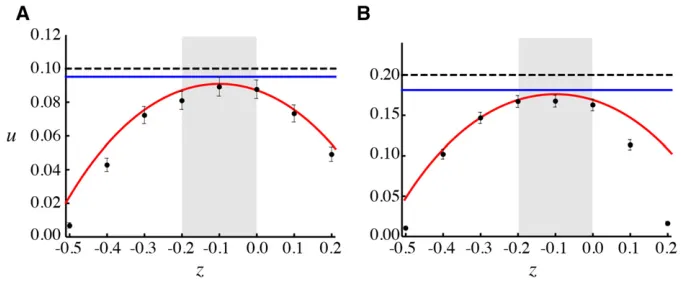
N= 100,fR= 0.5,bR¼bRR¼1000;dR¼dRR¼0:005;wR¼wRR¼1000;andsfM¼sMd ¼sdRM¼sdMM¼0;such that the fraction of haploids in the resident population is^rModelH ¼2=3:
sWFe ¼2sWFaveþð122h
wÞsw MM
2 ; (10a)
hWFe ¼ 2s WF ave 4sWF
aveþ ð122hwÞswMM
; (10b)
for the WF model. For an additive beneficial allele
ðhb¼hd¼hw¼1=2Þ;we havesMoran
e ¼2sMoranave ;sWFe ¼2sWFave; andhMoran
e ¼hWFe ¼1=2:
Given the above definitions for the variance effec-tive population size (Ne), the effective selection coeffi -cient (se), and the effective dominance coefficient (he), we regain the fixation probabilities derived above, uModeldiffusion;from thefixation probability in the classic dip-loid WF model (Kimura 1957, 1962; Crow and Kimura 1970, p. 427):
u*ðp0Þ ¼
Rp0
0 exp
22Nese
ð2he21Þp9
12p9 þp9dp9
R1
0exp½22Nesefð2he21Þp9ð12p9Þ þp9gdp9 :
(11)
For arbitrary dominance, the result must be numerically in-tegrated, but for additive mutationsðhb¼hd¼hw¼1=2Þ;
we have:
uModeldiffusionðp0Þ ¼ Rp0
0 exp
22NModel e sModele p9
dp9 R1
0exp
22NModel e sModele p9
dp9
¼12exp
22sModele NeModelp0
12exp22sModel e NModele
: (12)
Assuming weak positive selection on an initially rare mutation ðsModel
e NeModelp00Þ in a large population
ðsModel
e NeModel..1Þ;we obtain the classic approximation to thefixation probability,uModel
diffusionðp0Þ 2sModele NeModelp0:The result is the same as that obtained using branching process-es if we assume weak selection, as given by Equation 6 for the WF model:
uWFbranchuWFdiffusion 8^r WF
H ^rWFD
^
rWFH þ2^rWFD
22s WF
ave; (13a)
and by taking the Taylor series of Equation 2 to leading order in selectionðeÞfor the Moran model:
uMoranbranchuMorandiffusion
8^rMoranH ^rMoranD
^
rMoranH þ2^rDMoranhðdR=dÞ^rMoranH þ2ðdRR=dÞ^rMoranD isMoranave :
(13b)
We next turn to numerical analyses of these equations to better understand how thefixation probability depends on life history parameters of haploids and diploids.
Comparisons to numerical simulations
Similar haploid and diploid life histories:Wefirst consider the accuracy of these analytical approximations by com-paring the fixation probability to numerical simulations when the life history parameters are equivalent between haploid and diploid residents (bR=bRRanddR=dRRfor
the Moran model, wR=wRRfor the WF model). This
sce-nario may be appropriate for isomorphic species with mor-phologically similar haploid and diploid stages (e.g., the green alga Ulva, the brown alga Dictyota, the red alga Chondrus,etc.).
In Figure 1, we illustrate the fixation probability for the Moran model (A–C) and WF model (D–F) as a function of the average selection experienced by a rare allele,sModel
ave ;where selection acts only in the haploid phase (Figure 1, A and D; sb
MÞ or in the diploid phase (remaining panels; s
b
MM andh
bÞ;
assuming for simplicity that selection acts only through fer-tilityðsf
M¼s
d
M ¼s
d
RM ¼s
d
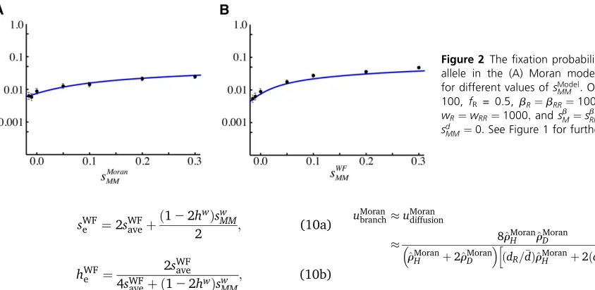
MM¼0Þ:Figure 2 represents thefi xa-tion probability for different values ofsModel
MM ;when selection
does not act on the allele while rare (i.e., the allele is fully recessive in diploids and has no selective benefit in haploids, sModel
ave ¼0Þin the Moran (A) and WF model (B). In Figure 3,
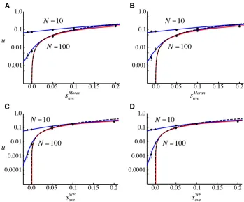
we illustrate how thefixation probability varies for a given total number of individuals,N.
The branching process approximation allowing for strong selection (solving numerically foruMoran
branchfrom Equation 2 and uWF
branch from Equation 5a with Equation D4) accurately pre-dicts thefixation probability from numerical simulations re-gardless of the strength of selection (red curve, see inset panels of Figure 1), but this method is valid only when the population size N is large and the average effect of a rare mutation is beneficial, f~MfRM.f~RfRR; failing when there
is no selection on a rare allele (Figure 2). As expected, ap-proximating the branching process results for weak selection
for different values ofsModel
MM :Other parameters:N= 100, fR = 0.5, bR¼bRR¼1000; dR¼dRR¼0:005;
wR¼wRR¼1000;andsbM¼s
b
RM¼sfM¼sdM¼sdRM¼
sd
MM¼0:See Figure 1 for further information.
(Equation 13) is accurate only when selection is weak (black dashed line in Figure 1).
By contrast, the diffusion equation (4a) with drift and diffusion coefficients (3) for the Moran model and (7) for the WF model provides a good approximation as long as selection is weak (Figure 1, Figure 2, and Figure 3, blue curves), even when the average effect of a rare mutation is not beneficial and/or the population size is small. Also, the diffusion well approximates the fixation probability when the mutation is fully recessive and has no effect in haploids (Figure 2), which is a case that cannot be handled by the branching process approximation because the fate of the allele is not determined while it is rare.
Because we have assumed equal death rates for haploids and diploids, thefixation probabilities behave similarly for the Moran (Figure 1, A–C) and WF models (Figure 1, D–F), except for the fact that the fixation probability is approxi-mately halved in the Moran model,uWF
diffusion2u Moran diffusion;due to the difference inNe(see Equation 8).
Different haploid and diploid life histories: We next con-sider thefixation probability in organisms whose life histories differ between haploid and diploid stagesðbR6¼bRR;dR6¼dRR
for the Moran model, andwR6¼wRRfor the WF model), as
would be appropriate for heteromorphic species (e.g., the green algaDerbesia, the brown algaMacrocystis, the red alga Porphyra,etc.). Again, both the branching process and diffu-sion approximations work well under the conditions assumed during their derivation (Figure 5). Thisfigure also compares the results to classical haploid-only or diploid-only models,
showing that the fixation probability in a haploid-diploid population differs dramatically as the frequency of haploids vs.diploids in the population varies.
We first discuss the case where the mortality rates of haploids and diploids are equivalent ðdR¼dRRÞ: With
equal death rates, haploids and diploids have the same expected life span in the Moran model, as is assumed in the WF model where all individuals die at each time step. In this case, the fixation probability of beneficial mutations with weak selection and a large population becomes
uMoran¼ 8r^Moran H r^
Moran D ð^rMoranH þ2^rMoranD Þ2
sMoran
ave for the Moran model and
uWF ¼ 8^rWF H ^r
WF D ð^rWFH þ2^rWFD Þ2
2sWF
avefor the WF model, using either
branch-ing processes or a diffusion approximation (Equation 13). We next compare thesefixation probabilities for haploid-diploid populations to the classic results for selection only in hap-loids (Moran:sH¼sfM=2þs
b
MþsdM;WF:sH¼sfM=2þswMÞvs.
selection only in diploids (Moran: sD¼ sbRMþsdRM; WF:
sD¼swRM), assuming selection is additive.
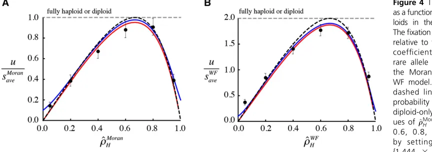
The fixation probability (13) reaches a maximum of uMoran¼ ðs
HþsDÞ=2 for the Moran model and uWF¼
ðsHþsDÞ for the WF model when ^rModelH ¼2=3 (Figure 4).
When haploids comprise two-thirds of a haploid-diploid pop-ulation, there is an equal number of alleles present in hap-loids and in diphap-loids, which maximizesNModel
e p0(minimizing drift for a newly arisen mutation), thereby maximizing the
fixation probability for a given total number of individuals. At this maximum, the fixation probability (Equation 13, black dashed curve in Figure 4) is the average of thefixation prob-ability in a fully haploid population (sHfor the Moran model
Moran model and (C and D) WF model, plotted as a function of (A and C) selection in haploids, and (B and D) selection in diploids withN = 10 or 100. Parameters: (A) sbM¼2sMoranave and s
b
RM¼s
b
MM¼0; (B)
sMb¼0; sbRM¼2sMoranave ; and hb¼0:5; (C)
sw
M¼2sWFaveandswRM¼swMM¼0;(D)swM¼0;
sw
RM¼2sWFave;andhw¼0:5:Other parameters:
fR = 0.5, bR¼bRR¼1000; dR¼dRR¼ 0:005; and sf
M¼sdM¼sRMd ¼sdMM¼0: See Figure 1 for further information.
and 2sHfor the WF model) and in a fully diploid population
(sDfor the Moran model and 2sDfor the classic diploid WF
model). In Figure 4, we explore a case where the fixation probability is the same in haplont and diplont populations (grey dashed curve), in which case thefixation probability in a haploid-diploid population under weak selection (13) is only the same if two-thirds of the population is haploid (black dashed curve). The simulation results tend to fall slightly below this expectation, however, due to the small population size and relatively large selection coefficients assumed (black dots in Figure 4).
When the fraction of haploids departs from two-thirds, however, thefixation probability decreases dramatically (Fig-ure 4), reaching zero when most individuals are haploids
ð^rModelH 1Þ or diploidsð^r
Model
D 1Þ:This sensitivity to the
relative proportions of haploids and diploids occurs because the new allele must be carried by both haploid and diploid individuals, in alternating generations, in a haploid-diploid population. Hence, when the ratio of haploids to diploids in the population is very skewed, the strength of random genetic drift is increased in whichever ploidy phase has fewer individuals.
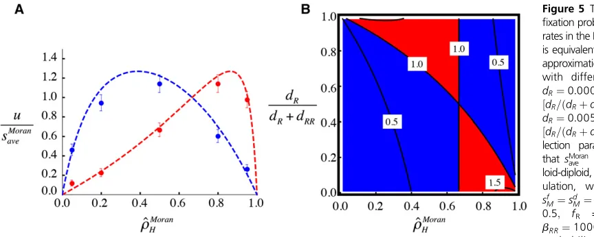
We next allow the mortality rates of haploids and dip-loids to differ as wellðdR6¼dRRÞ:As seen in Figure 5A, we
again find that the fixation probability approaches zero whenever the ratio of haploids to diploids is extremely skewed ð^rModelH near zero or one). With mortality rates
varying between the ploidy levels, however, the peakfi xa-tion probability no longer occurs atr^MoranH ¼2=3:As a con-sequence, increasing the mortality rate of haploids relative to diploids may increase or decrease thefixation probability of a beneficial mutation, depending on the overall popu-lation frequency of haploids. In Figure 5B, we illustrate the parameter space within which thefixation probability in a haploid-diploid population is larger than in a fully haploid and fully diploid population (red), or smaller than the two (blue), as a function of the frequency of haploids ðx-axis:r^MoranH Þ and the relative mortality rate
of haploidsðy-axis:dR=ðdRþdRRÞÞ:
At an intuitive level, beneficial alleles are better preserved and more likely tofix when the more common ploidy phase also has the lower mortality rate, allowing alleles to remain in this phase for longer.
Ploidally antagonistic selection:In this section, we consider cases where selection acts in opposite directions in haploid and diploid phases (ploidally antagonistic selection). The above derivations have not made assumptions about the sign of selection in each phase, although the branching process approximation assumes that thefixation probabil-ities in (1) are both positive. To assess the robustness of these approximations when selection acts in opposite di-rections in haploids and diploids, we setsu
M¼0:2þzand
su
RM¼ 2zðsModelave ¼0:1Þ foru2 fb;wgand varied the
de-gree of antagonism (z) in Figure 6.
The diffusion approximation (blue curves) applies only while selection in both phases is weak. The diffusion approx-imation depends only on the average strength of selection (see Equation 3b and Equation 7a) and fails to capture the large oscillations in allele frequency that occur between haploid and diploid phases whenzis large.
The branching process does, however, capture the decline in the fixation probability that occurs as the oscillations in selection across haploid and diploid phases increase in mag-nitude. When ploidally antagonistic selection becomes very extreme, however, selection no longer favors alleleMwhen it becomes common. We can measure selection onMonce com-mon as the difference infitness of M-bearingvs. R-bearing individuals relative to the now common genotypes,MMand M: 1
2 hð1þsu
RMÞ ð1þsu
MMÞ2 1iþ1
2
1 12su
M2
1;averaging across the two
phases. Selection only remains positive in Figure 6, favoring M when it becomes common, if z falls between20.377 and 0.177. Beyond these points, the branching process begins to break down because the loss orfixation ofMis no longer decided while it is rare. Indeed, once z extends beyond 20.432 and 0.232, both alleles MandR can invade when rare according to the branching process approximation in both the Moran and WF models. Beyond these values, we loids in the population ð^rModelH Þ:
Thefixation probability is measured relative to the average selection coefficient experienced by a rare allele ðuModel=sModel
ave Þ in (A) the Moran model and (B) the WF model. The horizontal gray dashed lines give the fixation probability in haploid-only and diploid-only populations. The val-ues of^rModelH of {0.05, 0.2, 0.4, 0.6, 0.8, 0.95} are obtained by setting bR¼wR equal to {1.444 3 106, 64000, 9000,
1777.78, 250, 11.08}. Selection parameters arefixed atsb
M¼s
b
RM¼swM¼swRM¼0:1; sfM¼sdM¼sdRM¼sdMM¼0;andhb¼hw¼0:5;withfR= 0.5, bRR¼wRR¼1000;anddR¼dRR¼0:005:See Figure 1 for further information.
expect ploidally antagonistic selection to maintain polymor-phism for extended periods of time [see bottom of Figure 6, A and B, inFile S1; the stochastic analog of the protected poly-morphism identified by Immleret al.2012].
In the WF model, a further complexity arises because of the fact that a mutation that appears in a haploid will only be in diploid offspring, haploid grand-offspring,etc., because of the assumption of completely nonoverlapping generations. This alternation can lead to the situation where the entire pop-ulation is composed of M haploids and RR diploids, fol-lowed in the next generation by R haploids and MM diploids; continuing to alternate until the population hap-pens to lose one genotype or the other. At that point, allele M tends tofix only when its geometric meanfitness
is higher:
ffiffiffiffiffiffiffiffiffiffiffiffiffiffiffiffiffiffiffiffi fM
2wMwMM q
. ffiffiffiffiffiffiffiffiffiffiffiffiffiffiffiffifR 2wRwRR q
;which requiresz,0.122. Because M is now in a different context,finding itself in MM diploids that are disfavored whenzis positive, the branching process fails to capture the probability offixation for large val-ues ofz.
Overall, wefind that our results continue to apply with ploidally antagonistic selection as long as selection in each phase is weak for the diffusion approximation and the fate of an allele is decided while it remains rare for the branching process approximation.
Discussion
Sexual organisms often exhibit complex life cycles alternating between different ploidy phases, with free-living haploid and diploid individuals. We develop a genetic model explicitly considering the population dynamics of haploid and diploid individuals by generalizing classical genetic models: the Moran model and the WF model. Using a branching process and a diffusion approximation, our work is thefirst to derive thefixation probability for organisms with haploid-diploid life cycles.
The fixation probability obtained by using branching processes (Equation 2),uModelbranch;provides a good approxima-tion to our simulaapproxima-tion results when the average effect of a mutation is beneficial ðsModel
ave .0Þ and the total population sizeNis sufficiently large, as long as ploidally antagonistic selection is not so strong that the allele becomes deleterious as it rises in frequency. On the other hand, thefixation prob-ability from the diffusion approximation (Equation 4a), uModel
diffusion;is accurate for both deleterious and beneficial mu-tations for both small and large populations, but only when selection is weak in each phase.
When average selection is weak, additive, and positive, and when starting from a single mutation, the branching process and diffusion approximations converge to Equation 13a for the WF model and Equation 13b for the Moran model. When the mortality rates are equal in haploids and diploids, the
fixation probability reduces in both models to:
uModel¼ 8^r Model
H r^ModelD
^
rModelH þ2^rModelD
2C Model
sModelave ; (14)
where CWF¼2 for the WF model and CMoran¼1 for the Moran model; reflecting the increased stochasticity in the Moran model, which samples both individuals to die and to give birth (all parents die in the WF model). Equation 14 demonstrates an important aspect of thefixation proba-bility in organisms with free-living haploid and diploid phases: beneficial alleles are less likely tofix in populations with skewed ratios of haploids to diploidsð^rModelH near zero or oneÞ:
This contrasts with classical results for haplont or diplont pop-ulations (Crow and Kimura 1970), where the other ploidy phase is assumed to be effectively infinite (no drift).
The“average effect”of selection, which averages selection across reproduction, fertilization, and mortality for both haploid and diploid phases, plays a key role in thefixation probability in haploid-diploid populations. Mutations can rates in the Moran model. (A) Panel is equivalent to the weak-selection approximation shown in Figure 3A with different mortality rates:
dR¼0:0005 and dRR¼0:005 ½dR=ðdRþdRRÞ 0:09(red), and
dR¼0:005 and dRR¼0:0005 ½dR=ðdRþdRRÞ 0:91(blue). Se-lection parameters are fixed so thatsMoran
ave is the same in a hap-loid-diploid, haplont, or diplont pop-ulation, with sbM¼s
b
RM¼0:05;
sf
M¼sdM¼sdRM¼sdMM¼0; hb¼ 0:5; fR = 0.5, and bR¼
bRR¼1000: (B) The fixation probability scaled to selection ðuMoran=sMoran
ave Þis shown as a function of^rMoranH (x-axis) anddR=ðdRþdRRÞ(y-axis). The blue region indicates when thefixation probability is less than that for both a haploid-only and diploid-only populationðuMoran=sMoran
ave ,1:0Þ:The red region indicates the region when thefixation probability is higher than both a haploid-only and diploid-only populationð1:0,uMoran=sMoran
ave Þ:See Figure 1 for further information.
have deleterious effects at one ploidy level, but not the other, and still be beneficial overall. Alternatively, such ploidally an-tagonistic selection can maintain polymorphism (Immleret al. 2012). In that case, the diffusion model can also be used with the mean and variance components derived here to obtain the time to loss of one or the other allele, or the stationary distri-bution, as well as thefixation probability.
Our results in a haploid-diploid population offer an in-teresting comparison to models with separate sexes (e.g., Crow and Kimura 1970; Hill 1979; Pollak 1990; Caballero 1995) or two patches (e.g., Maruyama 1970; Whitlock and Barton 1997; Whitlock 2003; Yeaman and Otto 2011). Con-siderfirst the case with separate sexes. To see the connection it is instructive to recalculate the variance effective popula-tion size using the method described in Crow and Kimura (1970), rather than the more formal derivation in Appendix D. In a population with two sexes consisting of M adult males and F adult females (both diploid) with allele frequenciesp♂andp♀, the average allele frequency among offspring is (p♂+p♀)/2 and the variance in allele frequency is [Var(p♂)+Var(p♀)]/4. This in turn equals14
pð12pÞ 2M þ
1 4
pð12pÞ 2F ;
assuming similar allele frequencies in the two sexes (p♂ = p♀ = p). Setting this to the variance expected in the classic diploid WF model without separate sexes, pð12pÞ=ð2NeÞ;we obtain the variance effective popula-tion sizeNe¼4MF=ðMþFÞ(Crow and Kimura 1970). For X-linked genes, the average allele frequency within the pop-ulation is instead (p♂+2p♀)/3, so that the expected variance is19
pð12pÞ
M þ
4 9
pð12pÞ
2F (note there is only one allele in males),
yielding Ne¼9MF=ð4Mþ2FÞ:One might initially assume that a haploid-diploid population would have a similar var-iance effective population size to anX-linked gene, but this is not the case. With a strict alternation of generations, a gene spends half of the generations in haploids and half in diploids, so the average allele frequency isðpHþpDÞ=2 (now
averaged over the alternation of generations), giving a var-iance in allele frequency of1
4
pð12pÞ
^
H þ
1 4
pð12pÞ
2^D and a variance
effective population size ofNe¼4H^D^=ðH^ þ2D^Þ(Equation 8b). This is most similar to the two sex, autosomal model but with M¼H^=2 and F¼D^:In both cases, descendants have an evolutionary history spent half in one type (males or haploids) and half in the other (females or diploids),
and the variance effective population size is sensitive to low numbers of either type. As a consequence, Ne is maximized in the haploid-diploid model when the phase with fewer genes (haploids) is relatively common
ðH^=ðH^þD^Þ 0:586Þ;whereasNeis maximized in the sex-linked model when the phase with fewer genes (males) is relatively rareðM=ðFþMÞ 0:414Þ:
The haploid-diploid model can also be thought of as a two-patch model, sharing similarities with models of subdivided populations (e.g., Tachida and Iizuka 1991; Gavrilets and Gibson 2002; Yeaman and Otto 2011). In the classical island and stepping stone models, thefixation probability in a sub-divided population is the same as that in an unsub-divided pop-ulation of the same total poppop-ulation size (Maruyama 1970). This assumes, however,“conservative migration,”where each population contributes to the dynamics of a metapopulation according to the local population size and where migration has no effect on the local population size (Whitlock and Barton 1997; Whitlock 2003). The haploid-diploid model, however, does not exhibit conservative migration. Rather, all haploids become diploids and vice versa (equivalent to a migration rate of 100% in the WF model). When one population is smaller (say haploids), that population has a much larger impact on the dynamics of the whole population because the larger pop-ulation (say diploids) descends entirely from it. Consequently, as we have shown here, thefixation probability of a haploid-diploid population does not obey Maruyama’s result for a single population, either haploid or diploid, with the same total number of individuals (Figure 4 and Figure 5).
By deriving the fixation probability for haploid-diploid populations, this work has extended classical population ge-netic results to organisms with an alternation of generations, allowing a better understanding of the role of stochasticity and drift in such species. Given that a large number of genes are expressed during both the haploid and diploid generations (Coelho et al.2007), the theoretical framework developed here also allows for the integration of selection of these “shared”(pleiotropic) genes across the life cycle.
Acknowledgments
We thank Ron Blutrich for help in the development of this manuscript. We also thank H. Otsuki, A. Sasaki, Y. Uchiumi, and (B) WF model, plotted as a function of the degree of ploidally antagonistic selection, z, where sModel
M ¼sModelave þz and sModelRM ¼2z: For small values ofz, selection remains direc-tional (gray box) but becomes ploidally antago-nistic outside this range. Parameters: (A)
sbM¼0:2þz; s
b
RM¼2z; hb¼0:5; and (B)
sw
M¼0:2þz;swRM¼ 2z;andhw¼0:5:Other parameters: fR = 0.5, bR¼bRR¼wR¼
wRR¼1000; dR¼dRR¼0:005; and sfM¼
sd
M¼sdRM¼sdMM¼0:See Figure 1 for further information.
of S.P.O., and two anonymous reviwers for helpful sugges-tions and discussions. This project was funded by a Grant-in-Aid from a Japan Society for the Promotion of Science (JSPS) postdoctoral fellowship for research abroad, a JSPS post-doctoral fellowship (16J05204) to K.B., and by a Natural Sciences and Engineering Research Council of Canada grant (183611) to S.P.O.
Literature Cited
Bell, G., 1994 The comparative biology of the alternation of gen-erations. Lect. Math Life Sci. 25: 1–26.
Bell, G., 1997 The evolution of the life cycle of brown seaweeds. Biol. J. Linn. Soc. Lond. 60: 21–38.
Caballero, A., 1995 On the effective size of populations with separate sexes, with particular reference to sex-linked genes. Genetics 139: 1007–1011.
Coelho, S. M., A. F. Peters, B. Charrier, D. Roze, C. Destombe et al., 2007 Complex life cycles of multicellular eukaryotes: new approaches based on the use of model organisms. Gene 406: 152–170.
Crow, J. F., and M. Kimura, 1970 An Introduction to Population Genetics Theory. Blackburn Press, Caldwell, NJ.
Destombe, C., M. Valero, P. Vernet, and D. Couvet, 1989 What controls haploid—diploid ratio in the red alga,Gracilaria verru-cosa?J. Evol. Biol. 2: 317–338.
Ewens, W. J., 2004 Mathematical Population Genetics 1: Theoret-ical Introduction. Springer Science & Business Media, New York. Gavrilets, S., and N. Gibson, 2002 Fixation probabilities in a
spa-tially heterogeneous environment. Popul. Ecol. 44: 51–58. Haldane, J. B. S., 1927 A mathematical theory of natural and
artificial selection, part V: selection and mutation. Math. Proc. Cambridge Philos. Soc. 23: 838–844.
Hill, W. G., 1979 A note on effective population size with over-lapping generations. Genetics 92: 317–322.
(Chlorophyta). J. Phycol. 46: 882–888.
Hirose, H., 1975 General Phycology, revised Ed. 2, Uchida Roka-kuho, Tokyo (in Japanese).
Immler, S., G. Arnqvist, and S. P. Otto, 2012 Ploidally antagonistic selection maintains stable genetic polymorphism. Evolution 66: 55–65.
Karlin, S., and H. E. Taylor, 1981 A Second Course in Stochastic Processes. Academic Press, New York.
Kimura, M., 1957 Some problems of stochastic processes in genetics. Ann. Math. Stat. 28: 882–901.
Kimura, M., 1962 On the probability offixation of mutant genes in a population. Genetics 47: 713.
Mable, K. B., and P. S. Otto, 1998 The evolution of life cycles with haploid and diploid phases. BioEssays 20: 453–462.
Maruyama, T., 1970 Effective number of alleles in a subdivided population. Theor. Popul. Biol. 1: 273–306.
Nagylaki, T., 1976 The evolution of one-and two-locus systems. Genetics 83: 583–600.
Otto, S. P., and T. Day, 2007 A Biologist’s Guide to Mathematical Modeling in Ecology and Evolution. Princeton University Press, Princeton, NJ.
Pollak, E., 1990 The effective population size of an age-structured population with a sex-linked locus. Math. Biosci. 101: 121–130.
Tachida, H., and M. Iizuka, 1991 Fixation probability in spatially changing environments. Genet. Res. 58: 243–251
Taylor, P. D., 1990 Allele-frequency change in a class-structured population. Am. Nat. 135: 95–106.
Whitlock, M. C., 2003 Fixation probability and time in subdivided populations. Genetics 164: 767–779.
Whitlock, M. C., and N. Barton, 1997 The effective size of a sub-divided population. Genetics 146: 427–441.
Yeaman, S., and S. P. Otto, 2011 Establishment and maintenance of adaptive genetic divergence under migration, selection, and drift. Evolution 65: 2123–2129.
Communicating editor: L. M. Wahl
The Moran model is a Markov process where the state of the population at timet+ 1 can be treated probabilistically given the frequencies of all genotypes,xðGTÞ;in the previous time step. At each time step, a single individual is chosen to die and one is chosen to give birth, so that the population size remains constant.
Wefirst choose an individual to die, weighting the chance that each type is eliminated by its mortality rate. Thus, the probability that an individual with genotype (GT) is eliminated from the population is
~
dðGTÞ¼
dðGTÞxðGTÞ
dRxRþdMxMþdRRxRRþdRMxRMþdMMxMM: (A1)
We then replace that individual with a birth chosen randomly from all of the spores and zygotes that could be produced by the remaining population at timet. Because we assume a large population size, we assume that the change in genotype frequency due to the death in this time step is negligible for common genotypes (this assumption is not made in the simulations or for rare genotypes in our analysis). The probability that a haploid spore is recruited is then proportional to the rate at which diploids reproduce by meiosis to produce either R- or M-bearing spores:
cR¼bRRxRRþ bRMxRM
2 ; (A2a)
cM¼bMMxMMþbRMxRM
2 : (A2b)
Given that resident and mutant gametes are produced at ratesgR¼bRxR=2 andgM¼bMxM=2;respectively, and accounting for
the probability of fertilization, the probability that a diploid zygote is recruited is:
cRR¼
fR
2
b2Rx2
R bRxRþbMxM;
(A3a)
cRM¼ fRþfM
2
bRbMxRxM bRxRþbMxM;
(A3b)
cMM¼
fM
2
b2Mx2
M bRxRþbMxM:
(A3c)
Overall, the probability that genotype (GT) is recruited into the empty site is:
qðGTÞ¼
cðGTÞ
cRþcMþcRRþcRMþcMM:
(A4)
To derive thefirst moment of mutant allele frequencyfluctuations, we calculate the conditional expected value for the change in any functionFof the random variable as
E h
DF!XðtÞ j!XðtÞ ¼!x i
¼E h
F!Xðtþ1Þ 2F!XðtÞ j!XðtÞ ¼!x i
; (A5)
where!XðtÞ ¼ ½XRðtÞ;XMðtÞ;XRRðtÞ;XRMðtÞ;XMMðtÞTand! ¼ ðx xR;xM;xRR;xRM;xMMÞT:
Using Equation A1 and (A4), the expected change in the number of individuals with genotype (GT), DXðGTÞðtÞ ¼XðGTÞðtþ1Þ2XðGTÞðtÞis:
E h
DXðGTÞðtÞ!XðtÞ ¼!x i
¼12~dðGTÞ
qðGTÞ2~dðGTÞ
12qðGTÞ
¼qðGTÞ2~dðGTÞ; (A6)
Note that Equation A6 can be rewritten as
E h
DXðGTÞðtÞX !ð
tÞ ¼!x i
¼gcðGTÞ2dðGTÞxðGTÞ
Ndmean ; (A7)
dRMxRMþdMMxMMÞ=N:
These expected changes in genotype frequencies can be used to track the dynamics of the system and determine its equilibrium properties.
Equilibrium
When the mutant allele is absent, the resident population approaches an equilibrium withH^haploids of genotypeR(xR) andD^
diploids of genotypeRR(xRR), with stochasticfluctuations around this point. Assuming the population size is large (dropping
terms of order 1/N), we can solve for the equilibrium number of haploids and diploids,
^
H¼^rMoranH NandD^ ¼r^MoranD N; (A8a)
using (A7), which yields^gbRRD^2dRH^ ¼0 and^g¼ ðdRH^þdRRD^Þ=½ðfRbRH^=2Þ þbRRD^;to obtain the frequencies:
^ rMoranH ¼
ffiffiffiffiffiffiffiffiffiffiffiffiffiffiffi
bRRdRR
p ffiffiffiffiffiffiffiffiffiffiffiffiffiffiffiffiffiffiffiffi fRbRdR=2
p
þ ffiffiffiffiffiffiffiffiffiffiffiffiffiffiffibRRdRR
p and^rMoranD ¼
ffiffiffiffiffiffiffiffiffiffiffiffiffiffiffiffiffiffiffiffi fRbRdR=2
p ffiffiffiffiffiffiffiffiffiffiffiffiffiffiffiffiffiffiffiffi fRbRdR=2
p
þ ffiffiffiffiffiffiffiffiffiffiffiffiffiffiffibRRdRR
p : (A8b)
Equation A8b emphasizes the fact that haploids are most common when diploids reproduce and/or die at a higher rate, and vice versa.
Appendix B: Fixation Probability in the Haploid-Diploid Moran Model Using a Branching Process Approximation
To derive thefixation probability of a mutant allele, wefirst apply the branching process approximation for a two-patch model (e.g., Yeaman and Otto 2011). Because the fate of a mutant allele is assumed to be determined while it is rare in a branching process approximation, we ignore homozygousMMmutants and consider only the change in number of haploid mutantsXM
and diploid mutantsXRM. As in Appendix A, we assume that the life cycle consists of the death of a single individual, followed by
the birth of an individual from the pool of haploid spores and zygotes that could be produced at that time step. In this birth step, we again assume that the population size is large enough that we can ignore the small change inqðGTÞthat occurs following the
death of an individual with one of the common genotypes.
When a single haploid mutant appears in the resident population, the numbers of individuals are xM= 1, xR¼H^21;
xRR¼D^;andxRM=xMM= 0. When a single diploid mutant appears in the resident population, we havexR¼H^; xM= 0,
xRR¼D^21;xRM= 1, andxMM= 0. Plugging these into Equation A1, the probabilities that a mutant individual is chosen to die
are:
~
dMjH¼
dM ^
dN and
~
dRMjD¼
dRM ^
dN; (B1)
where ^d¼dR^rHþdRR^rD (assuming the population is large) and otherwise residents are sampled to die (i.e., ~
dMjH¼12~dRjH2~dRRjH and~dRMjD¼12~dRjD2~dRRjDÞ:We add“|H”or“|D”to the subscript to clarify that we start with one
haploid or one diploid mutant individual.
When a single haploid mutant appears in the resident population, the expected number of zygotes is: cRRjH ¼
fRbRðH^21Þ 2
bRðH^21Þ
bRðH^21ÞþbM;cRMjH¼
fRþfM 2
bRbMðH^21Þ
bRðH^21ÞþbM;andcMMjH¼
fMbM 2
bM
bRðH^21ÞþbM:Because the diploid population consists solely ofRRindividuals, the rate of production of haploid spores is:cRjH¼bRRD^andcMjH ¼0:BecauseNis assumed to be very
large in a branching process approximation and homozygotes are rare, the probability that the sampled offspring will be of genotype (GT) given by Equation A4 is approximately:
qRMjH
ðfRþfMÞbM
2b^N andqMMjH0; (B2)
where^b¼fRbR 2 ^r
Moran
H þbRR^r
Moran
D :
When a single diploid mutant appears in the resident population, we have cRRjD¼fRbRH^=2; cRMjD¼cMMjD¼0;
cRjD¼bRRðD^21Þ þ ðbRM=2Þ;and cMjD¼bRM=2:Because Nis large and homozygous mutants rare, the probability that a
mutant offspring is sampled is:
2b^N
Letp0jHðp0jDÞequal the probability that a mutant allele introduced into a single haploid individual with genotypeM(single
diploid individual with genotypeRM) is lost from the descendant population at some point in the future. Assuming that its fate is determined before the homozygote mutantMMappears, that the population is at demographic equilibrium, and that the probabilities of loss are independent of each other; these probabilities satisfy the law of total probability, accounting for all possible death-birth transitions:
p0jH¼d~MjHþ~dRjH
12qRMjH
p0jHþd~RjHqRMjHp0jHp0jDþ~dRRjH
12qRMjH
p0jHþ~dRRjHqRMjHp0jHp0jD (B4)
when starting with one initialMhaploid, and
p0jD¼~dRMjDþ~dRRjD
12qMjD
p0jDþd~RRjDqMjDp0jHp0jDþ~dRjD
12qMjD
p0jDþ~dRjDqMjDp0jHp0jD (B5)
when starting with one initialRMdiploid. The probabilities offixation are then defined as the chance that loss does not occur:
p1jH¼12p0jHandp1jD¼12p0jD:Recalling the branching process assumption that the fate of the allele is determined while
the mutation is rare, the probability that a single mutant allele is chosen to die
~
dðGTÞ
or reproduceðqðGTÞÞremains roughly
constant during this period. The pair in Equation B5 can thus be solved to give thefixation probabilities:
p1jH¼
qRMjH
12~dMjH
2 ~dMjH~dRMjD
qMjDð12~dRMjDÞ qRMjH
12~dMjH
þ~dMjH
; (B6a)
p1jD¼
qMjD
12~dRMjD
2 ~dMjHd~RMjD
qRMjHð12d~MjHÞ qMjD
12~dRMjD
þ~dRMjD
: (B6b)
Because the population size is very large, the probabilities of death or recruitment of a mutantd~M=H;~dRM=D;qM=D;andqRM=Hare
very small. Hence, thefixation probabilities are well approximated by:
pMoranH ¼qMjDqRMjH2 ~
dMjHd~RMjD
qMjD
qRMjHþd~MjH
; (B7a)
pMoranD ¼qRMjHqMjD2 ~
dMjHd~RMjD
qRMjH
qMjDþ~dRMjD
: (B7b)
Plugging (B1), (B2), and (B3) into (B7) along with the frequency of haploids among residents, (A8b), we obtain (1). Furthermore, we can apply a Taylor expansion ineto Equation 1, assuming weak selection. Specifically, we plug (A8b) into (1) and rewrite f~ðGTÞ and fðGTÞ in terms of the life history parameters and the mutant’s effect on those parameters
e:g:; fM ¼fR
1þsMf
¼fR
1þe~sMf
:Carrying out the Taylor series, thefixation probability is then approximately
pMoranH 4dRR^r
Moran
D
dR^rMoranH þ2dRR^rMoranD s
Moran
ave ; (B8a)
pMoranD 2dR^r
Moran
H
dR^rMoranH þ2dRR^rMoranD s
Moran
ave : (B8b)
processes in the Moran model.
Appendix C: Fixation Probability in the Haploid-Diploid Moran Model Using a Diffusion Approximation
To derive thefixation probability from a diffusion approximation, we begin by deriving thefirst and second moments for the expected change in mutant allele frequency.
Separation of Timescales
Because the total number of individuals is held constant atN, dynamics forX(GT)are described by four variables. Transforming the original system of Equation A7 into the new variables,pM;dp;rH;andFD;we have equivalent dynamics for the expected
changes in the new variables. Applying a separation of timescales (e.g., Nagylaki 1976; Otto and Day 2007), we then calculate the slow dynamics for the change in frequency of mutant allelespM:The details of the calculations are given in a supplementary
Mathematicafile (File S1).
Letfhrepresent the expected change in each variableðh2 fpM;dp;rH;FDgÞacross one generation given the current state of
the population:
EDhðtÞj!XðtÞ ¼!x¼fh
e;pM;dp;rH;FD : (C1)
The exact functional form for each variable is provided inFile S1.
To approximate the above with weak selection, we apply a Taylor series expansion ineto Equation C1. To constant order
½Oð1Þ;we have:
fpM
0;pM;dp;rH;FD ¼gpMðrHÞdp; (C2a)
fdp
0;pM;dp;rH;FD ¼gdpðrHÞdp; (C2b)
frH
0;pM;dp;rH;FD ¼
2bRRdRRð12rHÞ22fRbRdRr2H
NfdRrHþdRRð12rHÞgffRbRrHþ2bRRð12rHÞg
; (C2c)
fFD
0;pM;dp;rH;FD ¼gFD
pM;dp;rH;FD ; (C2d)
(see detailed form of thegh functions in theFile S1). We assume that the population rapidly reaches a quasi-equilibrium
according to these equations, which are independent of selectionðe¼0Þand reflect ecological dynamics and the approach to Hardy–Weinberg. Solving for this quasi-equilibrium by setting Equations C2 to zero, we have the steady state approximations:
dp¼FD¼0 andrH ¼r^H;which givesfpMð0;pM;dp;rH;FDÞ ¼0 for anypM. Consequently, the population quickly approaches a state where there is a similar allele frequency between the haploid and diploid populationðdp0Þ;a Hardy–Weinberg ratio in
the diploid populationðFD0Þ;and a haploid-to-diploid ratio close to that in the resident population given by Equation (A8b)
ðrH^rHÞ:We refer to this as the quasi-equilibrium, to emphasize the point that the dynamics will still change slowly due to
selection.
After the state of the population approaches this steady state, the variables change over a longer timescale due to selection
½dp¼FD¼OðeÞandrH¼^rHþOðeÞ:To derive these slow dynamics, we setdp¼~dpe;FD¼~FDe;andrH¼^rHþr~Hein
Equa-tion C1 and perform a Taylor series expansion arounde¼0;now keepingOðeÞorder terms. Doing so, wefind that the change in allele frequency represents a closed variable system that does not depend on the dynamics of the other variables to this order:
E½DpMðtÞj!XðtÞ ¼! x MMoranp ðpMÞ ¼
pMð12pMÞ
n
2sMoranave þpM
h
122hbsb
MMþ
122hd
sdMM
io
2N
̑
d
^
d; (C3)
where the weighted mean mortality rate is^d¼r^HdRþ^rDdRRand the harmonic mean mortality rate isd̑¼2 .
1
dRþ 1
dRR
:
Appropriate Weight for the Average Allele FrequencypM
When we transform the variables using different allele frequency definitions, the dynamics of the allele frequency did depend on the other variables toOðeÞ:That is, defining the average allele frequency aspM¼apHþ ð12aÞpDwith an arbitrary weighting,
![Figure 1 ThesNon a linear scale whenresident population is(D4)], the weak-selection approximation to the branching process [black dashed; Moran from (13b); WF from (13a)], and the diffusion approximation[blue; Moran from (4a) with (3); WF from (4a) with (7](https://thumb-us.123doks.com/thumbv2/123dok_us/1524102.1186804/6.603.74.529.45.300/thesnon-whenresident-population-selection-approximation-branching-diffusion-approximation.webp)