Scholarship@Western
Scholarship@Western
Electronic Thesis and Dissertation Repository
8-17-2015 12:00 AM
Stochastic Stability and Uncertainty Quantification of Ring-based
Stochastic Stability and Uncertainty Quantification of Ring-based
Vibratory Gyroscopes
Vibratory Gyroscopes
Soroush Arghavan
The University of Western Ontario
Supervisor
Prof. Samuel F Asokanthan The University of Western Ontario
Graduate Program in Mechanical and Materials Engineering
A thesis submitted in partial fulfillment of the requirements for the degree in Master of Engineering Science
© Soroush Arghavan 2015
Follow this and additional works at: https://ir.lib.uwo.ca/etd
Part of the Computational Engineering Commons, and the Electro-Mechanical Systems Commons
Recommended Citation Recommended Citation
Arghavan, Soroush, "Stochastic Stability and Uncertainty Quantification of Ring-based Vibratory Gyroscopes" (2015). Electronic Thesis and Dissertation Repository. 2986.
https://ir.lib.uwo.ca/etd/2986
This Dissertation/Thesis is brought to you for free and open access by Scholarship@Western. It has been accepted for inclusion in Electronic Thesis and Dissertation Repository by an authorized administrator of
STOCHASTIC STABILITY AND UNCERTAINTY QUANTIFICATION OF
RING-BASED VIBRATORY GYROSCOPES
(Thesis format: Monograph)
by
Soroush Arghavan
Graduate Program in Mechanical and Materials Engineering
A thesis submitted in partial fulfillment
of the requirements for the degree of
Masters of Engineering Science
The School of Graduate and Postdoctoral Studies
The University of Western Ontario
London, Ontario, Canada
c
Effect of stochastic fluctuations in angular velocity on the stability of two DOF ring-type MEMS gyroscopes is investigated. The governing Stochastic Differential Equations are dis-cretized using the higher-order Milstein scheme in order to numerically predict the system response assuming the fluctuations to be white noise. Simulations via Euler scheme as well as a measure of Largest Lyapunov Exponents are employed for validation purposes due to lack of similar analytical or experimental data. The stability investigation predicts that the threshold fluctuation intensity increases nonlinearly with damping ratio. Under typical gyroscope oper-ating conditions, nominal input angular velocity magnitude and mass mismatch appear to have minimal influence on system stability.
Furthermore, construction, electrical improvements, testing and troubleshooting of a macro-scale ring-type gyroscope prototype is completed. Experiments have been conducted in order to investigate the linearity of system response, system behavior when subjected to environ-mental fluctuation in angular rate as well as the effects of angular rate and mass mismatch on system natural frequency. It is shown that the system natural frequency decreases with input angular rate and mass mismatch. It is also revealed that the system exhibits a more efficient damping behavior when subjected to stochastic speed fluctuations with fixed intensity at higher input angular rates.
Acknowledgements
I am forever in debt to my supervisor Professor Samuel F. Asokanthan who kindly provided me with guidance in the arduous path of research and introducing me to an exciting research field. I owe my knowledge to him and I thank him for helping me in this thesis which was made possible through him.
I would also like to thank the National Sciences and Engineering Research Council (NSERC) of Canada Discovery Grant and The University of Western Ontario for the Western Graduate Research Scholarship (WGRS) for supporting this thesis.
my caring father Mohammadhassan
and my wise and motivating brother Sina.
I would not have been here without your love and support.
I have been blessed with the gift of a cherished family.
Contents
Acknowlegements iii
List of Figures viii
List of Tables x
Nomenclature xi
1 Introduction and Literature Survey 1
1.1 Introduction . . . 1
1.2 Literature Review . . . 2
1.2.1 A Short History of Gyroscopes . . . 2
1.2.2 Vibrating String . . . 5
1.2.3 Mass-Spring . . . 5
1.2.4 Tuning Fork . . . 6
1.2.5 Vibrating Shell . . . 6
1.2.6 Ring-type . . . 7
1.3 Thesis Objectives . . . 13
1.4 Thesis Outline . . . 14
2 Governing Equations 16 2.1 Introduction . . . 16
2.2 Model Description . . . 16
2.5 Closure . . . 23
3 Stochastic Model Incorporating Uncertainty in Input Angular Rate 25 3.1 Introduction . . . 25
3.2 Gaussian White Noise . . . 26
3.2.1 Stochastic Calculus . . . 26
3.3 Stochastic Fluctuation in Angular Rate . . . 27
3.4 Itˆo-Taylor Expansion . . . 30
3.5 Lyapunov Characteristic Exponent . . . 34
3.6 Closure . . . 35
4 Stability Analysis Using Numerical Methods 36 4.1 Introduction . . . 36
4.2 Numerical Predictions . . . 37
4.3 Parametric Study . . . 42
4.4 Closure . . . 44
5 Experimental Results 46 5.1 Introduction . . . 46
5.2 Experimental Setup . . . 47
5.3 Experimental Results and Discussion . . . 53
5.4 Stochastic Fluctuation in Angular Rate . . . 61
5.5 Closure . . . 64
6 Conclusion 65 6.1 Thesis Contributions . . . 66
6.2 Recommendations for Future Research . . . 67
Bibliography 69
A Derivation of Equations of Motion 74
A.1 Introduction . . . 74
A.2 Energy Equations . . . 74
A.3 Natural Frequencies . . . 76
A.4 Normalized Equations of Motion . . . 78
B Matlab Codes 81 B.1 Introduction . . . 81
B.2 Time Series Simulation . . . 81
B.3 Largest Lyapunov Exponent Calculation . . . 85
B.3.1 Calculating Mutual Average Information . . . 85
B.3.2 Calculating Mean Period . . . 87
B.3.3 Calculating Lyapunov Exponents . . . 88
B.3.4 Finding Largerst Lyapunov Exponent of The Simulated Time Series . . 90
C Experimental Setup 92 C.1 Startup Procedure . . . 95
C.1.1 Rate Table Initial Startup . . . 96
C.2 Shutdown Procedure . . . 98
Curriculum Vitae 108
1.1 A simple gyroscope. (Scarborough, 1958) . . . 3
1.2 Schematics of a spring-mass type gyroscope (Reproduced from Clark, 1999) . . 6
1.3 SEM view of a tuning fork gyroscope. (G¨unthner et al., 2006) . . . 7
1.4 SEM view of a polysilicon ring gyroscope 1 mm in diameter. (Ayazi and Najafi, 1998) . . . 8
1.5 Schematic of a BAW inertial sensor. (Kempe, 2011) . . . 10
2.1 Schematic of the rotating ring geometry. (Cho, 2005) . . . 17
2.2 Visualization of the second flexural modes of the ring. (Cho, 2005) . . . 17
2.3 Variation of natural frequencies with angular rate with non-uniform mass as-sumption. (Cho, 2005) . . . 23
4.1 Example of stable time response. . . 37
4.2 Example of marginally stable time response. . . 39
4.3 Example of unstable time response. . . 39
4.4 Under-prediction of results by Euler scheme in a marginally stable case. . . 40
4.5 Under-prediction of results by Euler scheme in a marginally unstable case. . . . 41
4.6 Stability boundary in theµ-ζspace (Ω =2πrad/s). . . 43
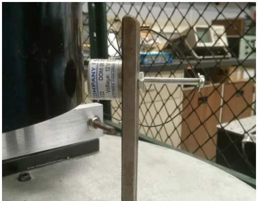
5.1 Experimental setup . . . 48
5.2 Configuration of an electromagnetic exciter. . . 49
5.3 Configuration of the Eddy-Current probes. . . 49
5.5 Implementation of stochastic angular rate fluctuation setup. . . 51
5.6 Block diagram representation of the experimental setup. . . 52
5.7 Schematic representation of the experimental setup. . . 53
5.8 Natural frequency shift in the Cross Spectrum Magnitude diagram due to an-gular rotation. . . 54
5.9 Linearity of nodal and anti-nodal measurements. . . 55
5.10 Suggested locations for mass anomaly. . . 56
5.11 Anti-nodal measurements of time response for 2.5% mass mismatch located at points 1 to 3. . . 57
5.12 Anti-nodal measurements of time response for 2.5% mass mismatch located at points 4 to 6. . . 58
5.13 Nodal measurements of time response for 2.5% mass mismatch. . . 58
5.14 Variation of natural frequency with mass mismatch - experimental results. . . . 59
5.15 Effects of fluctuations in angular rate on raw sensor measurements,Ω =0 rad/s. 61 5.16 Effects of fluctuations in angular rate on raw sensor measurements,Ω =2πrad/s. 62 5.17 Variation of output standard deviation with angular rate. . . 63
C.1 Experimental setup. . . 92
C.2 Experimental setup close-up . . . 93
C.3 Configuration of an electromagnetic exciter. . . 94
C.4 Configuration of the Eddy-Current probes. . . 94
C.5 Layout of a junction box. . . 95
C.6 Block diagram representation of the experimental setup. . . 99
C.7 Schematic view of the experimental setup. . . 100
C.8 Wiring diagram for single sensor operation. . . 101
C.9 Wiring diagram for dual sensor operation. . . 102
C.10 Front panel of the LabView script. . . 106
1.1 Grade requirements of gyroscopes (Yazdi et al., 1998) . . . 4
1.2 Applications of gyroscopes with estimated typical grades . . . 9
2.1 Physical properties of the MEMS ring . . . 22
4.1 Summary of LLE values for predicted time responses. . . 42
4.2 Variation of system natural frequencies with input angular rate. . . 44
4.3 Variation of system natural frequencies with mass mismatch. . . 44
5.1 Physical properties of the experimental ring . . . 48
5.2 Summary of measurements with concentrated mass located at different points on the ring. . . 60
C.1 Input 37-pin connection pinout (Rate table J100 and J101) . . . 103
C.2 Output 37-pin connection pinout (Rate table J102 and J103) . . . 104
C.3 ECL134 15-pin output connection pinout . . . 105
Nomenclature
α Rotational coordinate
δm Mass mismatch
δ(t) Dirac’s delta function
γ Ring model constant
κ1 Ring model constant κ2 Ring model constant
M Mass matrix
q Flexural generalized coordinate vector
µ Relative noise intensity measure
µ0 White noise intensity
Ω Angular rate
ω Frequency, Excitation frequency
ω01 Natural frequency of the first degenerate configuration of the second flexural mode
shape
shape
Φ Variable space
ρ Density
σ Stress component
σa Averaged standard deviation
v Velocity vector
ε Strain component
ξ White noise
ζ Damping ratio
A Cross-section area
a[X(t)] Drift coefficient
b Axial thickness
b[X(t)] Diffusion coefficient
D Damping matrix
d Number of dimensions in Milstein scheme
E Young’s elasticity modulus
F Generalized excitation force vector
f External force component
f1 Excitation force amplitude
G Gyroscopic matrix
h Radial thickness
I Mass moment of inertia
K Stiffness matrix
k Stiffness component
m Number of independent Wiener processes
N Normal distribution
n Mode shape number
O Terms in the order ofδt3/2or higher
q Flexural generalized coordinate
r Mean radius
S Power spectral density function
T Time interval
u Displacement
W Brownian motion, Wiener process
X Stochastic process
Introduction and Literature Survey
1.1
Introduction
The ancient civilizations designed a simple toy called a ”top” for the sole purpose of entertain-ment, unaware of the applications of the device in the millennia to come. The invention of the spinning top opened the door to exquisite, then unimaginable advancements in low-cost high-accuracy navigation devices used worldwide in a diverse list of applications from long-haul transportation to entertainment. A wide variety of gyroscopic devices have been developed in the past century in order to quantify rotation and, essentially, simplify navigation.
In the past two decades, the world of Micro Electro-Mechanical Systems (MEMS) offered un-precedented opportunities in reducing the weight, size, production cost and power consumption of the sensors as well as increasing their accuracy in by omitting unnecessary moving parts and fluids. It was only logical that MEMS methods were applied to gyroscopes and gave birth to a new range of navigation devices. Although these devices offer countless possibilities, they are still prone to sources of error such as drift, effects of temperature change and unwanted vibration.
Chapter1. Introduction andLiteratureSurvey 2
Laboratory at Western University and focuses on a modern type of MEMS gyroscopes called the ring-type gyroscopes. In an effort to model and study the effects of environmental fluctu-ations in angular rate of ring gyroscopes, stochastic methods are utilized and integrated using numerical methods.
Although ring-type gyroscopes have been studied and manufactured in MEMS scale, more research needs to be done on the behavior of MEMS and macro-scale ring-type gyroscopes and problems associated with this class of devices. For this purpose, an experimental macro-scale prototype previously developed by Cho (2009) has been completed and complementary experiments were conducted in order to visualize the behavior of the device and the effects of low natural frequencies associated with such macro-scale devices.
1.2
Literature Review
1.2.1
A Short History of Gyroscopes
Germany) and Johnson (1832, United States). The orientation of the wheel stayed consistent, therefore confirming that the Earth is rotating constantly since the supporting gimbal is directly connected to the Earth (Foucault, 1852). The device acquired the name ”gyroscope”, from the Greek words ”gyros” (revolution) and ”skopein” (to see); a device that allows the user to see the revolution of the Earth. Although the word ”gyroscope” is used by some authors exclu-sively for rotary sensors with spinning wheels, it can be generally used for any device that is used to demonstrate or measure rotation (Lawrence, 1993). George M. Hopking, American inventor, employed an electric motor to maintain the angular velocity of the wheel at any de-sired speed in 1878. An example of this type of gyroscopes can be seen in Figure 1.1. In 1898, Ludwig Obry patented a torpedo steering mechanism that operated based on gyroscopic inertia which might have inspired Elmer A. Sperry, who developed the first automatic airplane pilot using gyroscopes and the first gyro-stabilizer for reducing roll in ships (see Lawrence, 1993; Scarborough, 1958).
Simple Gyroscope
( P fut t<.t g r up h co urt es,y S,p er r y G y r rt s u.t 1 t c C rL.)
Figure 1.1: A simple gyroscope. (Scarborough, 1958)
perfor-Chapter1. Introduction andLiteratureSurvey 4
mance, namely rate, tactical and inertial grade, where the inertial grade provides the highest accuracy possible while the rate grade is used for low-accuracy demanding applications. Table 1.1 displays the different grades of gyroscopes and the requirements that need to be met for categorizing a device under each grade.
Specification Rate Grade Tactical Grade Inertial Grade Angle Random Walk (deg/
√
hr) >0.5 0.5∼0.05 <0.001 Bias Drift (deg/hr) 10∼1000 0.1∼10 <0.01 Full Scale Range (deg/s) 50∼1000 >500 >400 Dynamic Range (dB) 40 100 100
Noise (deg/s.√Hz) >0.1 0.5∼0.05 <0.001 Absolute Accuracy (%) 0.1∼1 0.01∼0.1 <0.001 Bandwidth (Hz) >70 ∼100 ∼100 Table 1.1: Grade requirements of gyroscopes (Yazdi et al., 1998)
The most usual form of a gyroscope was a mechanical device consisting of a heavy flywheel rotating at high speeds until mid 1950s. These types of gyroscopes formed the majority of navigation devices in vessels (Kempe, 2011; Scarborough, 1958). New types of gyroscopes emerged beginning in the 1950s with the introduction of the Sperry rate Gyrotron (Morrow, 1955) opening the way to new classes of angular rate measurement devices that would not fit under the conventional definition of a gyroscope. Various types of gyroscopes have been devel-oped ever since for specific range of applications, such as angle and angular rate measurement, remote sensing, photogrammetry, terrestrial surveying and terrain profiling (Jekeli, 2001). In 1963, a new class of gyroscopes were born with the introduction of Ring Laser Gyroscopes (RLG) and Fiber Optic Gyroscopes (FOG). This class of gyroscopes which take advantage of the phase shift of light beams, commonly known as the Sagnac effect, are able to measure an-gular rate with exceptionally high accuracy and form the majority of inertial grade gyroscopes (Loukianov et al., 1999).
referred to as vibratory gyroscopes have been developed in pursuit of reducing the production cost and size of the sensors. However they did not attract the attention of the scientific com-munity until the rise of MEMS devices due to apparent lack of advantages over conventional gyros. With the introduction of MEMS devices, a unique characteristic of the vibratory gyros gave popularity to these sensors which is feasibility of production in micro-scale. Ever since, vibratory angular rate sensors have been the focus of researchers with the hope to develop more cost-effective and accurate devices. This research has led to development of several types of vibratory gyros including the vibrating string, mass-spring and vibrating shell resonator gyro-scopes which currently fall under the rate or tactical grade accuracy classification.
1.2.2
Vibrating String
The vibrating string gyro, as the name suggests, consists of an oscillating string. The string is fixed on both ends and the vibration plane of the string tends to remain stationary in case the supports rotate about the string axis (Quick, 1964). Quick, in 1964, realized that the Coriolis acceleration causes the vibration to be coupled into the plane perpendicular to the vibration plane and hence the vibration plane appears to not be affected by the rotation. Quick designed an apparatus which measures the coupling due to rotation and essentially acts as an angular measurement sensor.
1.2.3
Mass-Spring
This type of gyroscopes usually contains a proof mass oscillating along the X-axis using a driving force (FD) with the frame free to rotate about theZ-axis as shown in Figure 1.2. Coriolis
force FC, due to rotation combined with oscillation results in deflection of the proof mass in
Chapter1. Introduction andLiteratureSurvey 6
Figure 1.2: Schematics of a spring-mass type gyroscope (Reproduced from Clark, 1999)
1.2.4
Tuning Fork
Rotation of a vibrating tuning fork about its base produces periodically varying Coriolis forces along the rotation axis. The variations in the angular rate can be qualitatively explained through conservation of angular momentum with the fork rotating more rapidly when the tines are closer to each other and the fork rotating more slowly when the tines are apart (Morrow, 1955). Hence, forcing the fork to rotate about its axis at a steady speed results in the varying motion of the tines which can be calibrated against the angular speed of the base. An example of a MEMS tuning fork gyroscope under a Scanning Electron Microscope (SEM) is shown in Figure 1.3.
1.2.5
Vibrating Shell
er-Figure 1.3: SEM view of a tuning fork gyroscope. (G¨unthner et al., 2006)
ent temperature sensitivities of the natural frequencies of the two modes. Vibrating shell gy-roscopes, however, overcome this problem by taking advantage of two identical mode shapes. Bryan (1890) analyzed the vibration of cylindrical and bell-shaped shells using a wine glass analogy. Bryan noted that a wine glass produces a pure and continuous tone when struck. However, twisting the wine glass around results in audible beats demonstrating that the nodal meridians do not remain fixed in space. Furthermore, Bryan concludes that since the beats can still be heard with the observer turning around while holding the vibrating glass, the nodes do not rotate with the same angular velocity as the glass or the observer.
1.2.6
Ring-type
sus-Chapter1. Introduction andLiteratureSurvey 8
penders (Maluf and Williams, 2004). This type of gyros gained popularity for their minimal drift to temperature fluctuation and high sensitivity to rotation. Moreover ring-type and in gen-eral the vibrating shells gyros exhibit higher immunity to unwanted environment vibration as opposed to e.g., tuning forks due to their weak interaction with the supporting structure (see Asokanthan et al., 2006; Lawrence, 1993).
Ring-type vibratory gyroscopes rely on Coriolis effect for operation similar to other types of modern angular rate sensors with the exception of ring-laser sensors. A ring-type angular rate sensor is usually composed of a thin, light-weight ring, an exciter and a sensor. An example of a MEMS ring gyroscope can be seen in Figure 1.4. Vibration in a certain vibratory mode is excited in the ring using an exciter. Coriolis forces induced in the ring during rotation of the ring cause the excited ring to shift vibration into the next resonance mode. A well-placed sensor is able to detect the resultant shift and the sensor output is then calibrated against the rotation (Kempe, 2011).
More recently, the advancements in the fields of micro-machining and Micro Electro-Mechanical Systems (MEMS) have enabled development of gyroscopes and accelerometers in a small package. Low power consumption, small size, low manufacturing cost as well as moderate accuracy are the main advantages offered by MEMS angular rates sensors which makes them ideal for usage in everyday and practical applications. MEMS packages are used nowadays in vehicles for applications such as designing active suspension and navigation, in cameras for image stabilization and in consumer electronics (such as smartphones) for a range of applica-tion from navigaapplica-tion to entertainment (Abedin, 2014). Table 1.2 shows the typical applicaapplica-tions of a MEMS inertial sensor with the estimated grade requirements (S¨oderkvist, 1994; Yates, 1999).
Application Range Accuracy Grade Automotive Safety 50∼200◦/s 1∼10◦/s Rate
Consumer 50∼100◦/s 0.5∼ 2◦/s Rate Medical 20∼100◦/s 0.1∼ 2◦/s Rate/Tactical Industrial 10∼ 50◦/s 0.01∼0.2◦/s Tactical
Table 1.2: Applications of gyroscopes with estimated typical grades
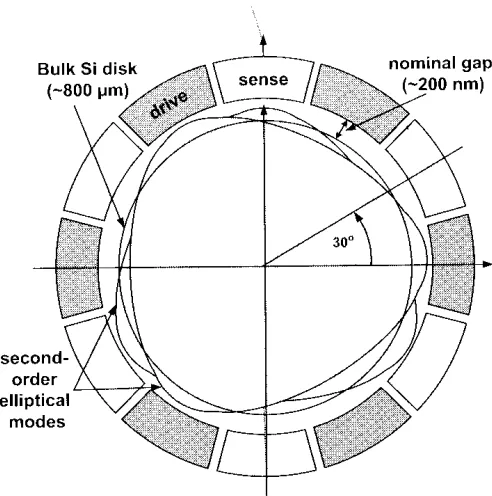
MEMS-based sensors primarily fall in the rate grade. Improvements in accuracy as well as their drift performance are warranted before they can be accepted as a true tactical or inertial grade device. To this end, several recent research as well as development efforts are underway. In the recent years, another type of sensors similar to ring gyroscopes called the Bulk Acoustic Wave (BAW) inertial sensors have been developed by Ayazi and Johari (2009) and currently in production by Qualtr´e Inc. BAW sensors are composed of a silicon disk which is manufactured in the HARPSS process and detect energy transfer as a result of rotation between two modes of high frequency (1 to 5 MHz) of the disk. BAW sensors offer full-scale ranges of 300∼ 3000◦/s
as well as temperature sensitivities as low as 0.05◦/s/◦C. A schematic of a BAW inertial sensor
Chapter1. Introduction andLiteratureSurvey 10
Figure 1.5: Schematic of a BAW inertial sensor. (Kempe, 2011)
Although the operating principles of the ring-type gyroscopes are fairly simple, complication might arise during typical manufacturing and operating conditions. Stability of the sensor is compromised when the device is subjected to disturbance caused by environmental fluctua-tions. Furthermore, development of a perfectly uniform ring is improbable resulting in non-uniform mass distribution of the ring, called mass mismatch. Introduction of mass mismatch affects the natural frequencies of the ring and essentially the operation as well as accuracy of the gyroscope. Hence, the main objective of the present thesis is assessment of dynamic sta-bility of MEMS-based ring-type vibratory gyroscopes under external disturbance as well as design and production of a macro-scaled prototype for the purposes of studying the physical and vibratory characteristics as well as the general behavior of the device.
motion was studied by Eley et al. (2000). Focusing on the system stability, a method for in-vestigating the stability of a linear gyroscopic system via a model of a rotating beam has been developed by Kammer and Schlack Jr. (1987). Recently, stability of a ring-based gyroscope when it is subjected to harmonic perturbation in angular rate has been studied via the method of averaging (Asokanthan and Cho, 2006). Although harmonic vibration may be a simple ap-proximation useful for modeling angular speed fluctuation emanating from the environment, white noise, which covers a wide range of frequencies, may be a more realistic representa-tion. Hence, introduction of the white noise is envisaged to aid in a more accurate prediction of the dynamic behavior of these devices as well as the physical systems they are mounted on. Asokanthan and Wang (2009) studied the effects of angular rate perturbations on mass spring systems using the second moment stability criteria and the method of averaging. The present investigation focuses on the dynamic stability of ring-structure gyroscopes based on their dynamic response, considering random perturbation in input angular velocity.
One of the most important factors that affect the operation of a ring gyroscope is deviation of the geometry from the intended axisymmetric design. Imperfections could occur mostly during the manufacturing stage. Non-uniformities in mass result in high levels of mechanical coupling and reduced secondary response which in return limits detection of low angular rates. To this end, previous research has shown that near-perfect aspect ratios are achieved using deep reactive ion etching as well as finer line photolithography is the fabrication process of silicon rings (Harris et al., 1998).
In another effort to increase the accuracy of ring gyroscopes Wang et al. (2010) designed and fabricated a sensor with harsh environmental conditions in mind. The final product demon-strated a low frequency split of 0.5 Hz between the sensing mode and driving mode frequencies due to high symmetry. Furthermore, it was shown that the frequency split remains consistent under different environmental conditions.
envi-Chapter1. Introduction andLiteratureSurvey 12
ronmental fluctuations on ring-type gyroscopes through numerical simulation. The developed schemes take advantage of the equations of motion for the ring-type gyroscopes which have been developed by Asokanthan and Cho (2006) based on the previous work by Huang and Soedel (1987). The present study further extends the work performed by Asokanthan and Cho (2006) for the periodic fluctuation by introducing a random perturbation in the angular rate. For this purpose, considering the random fluctuation, the governing equations that represent the motion of the gyroscopic system under investigation are written in the form of a system of standard Stochastic Differential Equations (SDE).
It is known that closed-form analytical solutions cannot be obtained for this class of systems owing to their highly non-differentiable character of the realization of the Wiener process (Higham, 2001). In the present study, the higher-order Milstein scheme is employed to sim-ulate the time response. The stochastic response of ring-based gyroscopes is then quantified for certain parameters of interest. The stability analysis is then performed based on the simu-lated responses so that the stability behavior of this class of gyroscopes can be predicted. To this end, an algorithm for computing the characteristic Lyapunov exponents of the response have been employed for validating the stability predictions via the stochastic response. Effects of damping and angular speed fluctuation magnitude on system stability have been quantified for different input angular velocities. In addition, these effects have also been quantified for a parameter that represents the non-uniformity in ring mass distribution.
1.3
Thesis Objectives
Although vibratory sensors are manufactured for common applications in MEMS-scale, it is not feasible to study the effects of environmental fluctuations on a MEMS-scale sensor due to the complexities of changing the geometry of the ring as well as selection of suitable mea-surement devices for a rotating MEMS ring. Moreover, numerical simulation of such devices poses another problem due to the barriers caused by the limitations of analytical and numerical methods. Considering the problem in hand, the present thesis aims to:
• Introduce environmental fluctuations in the input angular rate of ring-type vibratory gy-roscopes by employing a white noise function and develop the corresponding stochastic differential equations of motion considering the newly introduced noise intensity vari-able.
• Develop the required numerical tools using the available schemes in order to numeri-cally solve the resulting SDE and apply the developed scheme to the SDE. For this pur-pose, the goal is to employ the higher-order available schemes in order to obtain a novel method with higher accuracy than the simpler schemes and to implement the developed higher-order numerical equations using a Matlab script and validate the results against the commonly-used schemes using Largest Lyopunov Exponents stability assessment tools.
Chapter1. Introduction andLiteratureSurvey 14
• Develop a macro-scale ring-type vibratory sensor prototype using the experimental project previously initiated by Cho (2009). The project agenda includes development of reliable wiring of the device, installation and testing of sensors, development of a LabView script for data acquisition, monitoring and analysis, development of an instruction manual for safe operation and maintenance of the device as well as implementation of safety mea-sure to enmea-sure safe operation of the experimental setup.
• Conduct experiments on the bifurcation of natural frequencies of a ring-type gyroscope and demonstrate the reduction of natural frequency due to angular rotation as well as the non-linear behavior of the macro-scale device as a result of large-amplitude vibrations and relatively low natural frequency close to operating angular rates.
• Investigate the effect of increased non-uniform mass distribution due to manufacturing defects on natural frequencies of the system and compare the results with previous the-oretical analysis in literature. Furthermore, the goal is to demonstrate the effects of fluctuations in angular rate on system behavior which can be used to further the exper-imental research into dynamic stability of macro-scale systems similar to the numerical study performed in the present thesis.
1.4
Thesis Outline
The present thesis is comprised of a numerical and an experimental study on the behavior of ring-type gyroscopes. Conforming to the objectives of the thesis, the thesis is presented in the following chapters:
Differential Equations.
Chapter 3reviews the stochastic calculus tools required in order to numerically solve the de-veloped equations. Moreover, the common numerical schemes are introduced, explained and compared and the higher-order Milstein numerical scheme is applied to the stochastic diff eren-tial equation at hand.
The results of the numerical study are discussed inChapter 4. This chapter starts by validating the developed method using Largest Lyapunov Exponent method and comparing the method with the more commonly used Euler method. Times responses obtained using the Milstein method are analyzed and a parametrical study is performed in order to obtain an intensity threshold for fluctuations in angular rate using a prescribed system damping ratio. Effects of angular rate and mass uniformity on system natural frequencies are also discussed inChapter 4and the discussion on the findings is ensued.
The details of the experimental setup are discussed in Chapter 5 as well as the experimental results on effects of angular rate, environmental fluctuations and mass uniformity on system natural frequency.
Chapter 2
Governing Equations
2.1
Introduction
The governing equations for the system developed using Hamilton’s principle by Cho (2005) have been employed to study the effect of stochastic fluctuation in input angular rate. Complex Fourier series are then used to derive the modal shapes of the ring. In this chapter, the employed model is reviewed in order to better understand the experiments and implementation of the numerical models.
2.2
Model Description
The ring is assumed to be of uniform rectangular cross section of widthband sufficiently thin with the ratio of radial thickness hto mean radius r, i.e., (h/r)2 << 1 (see Love, 2013). The
material chosen for the ring is assumed to be isotropic and homogeneous while the transverse shear deformation of the ring is considered negligible in accordance with the thin ring assump-tion and the Euler-Bernoulli theory (see Soedel, 2004). It is assumed that the circumferential
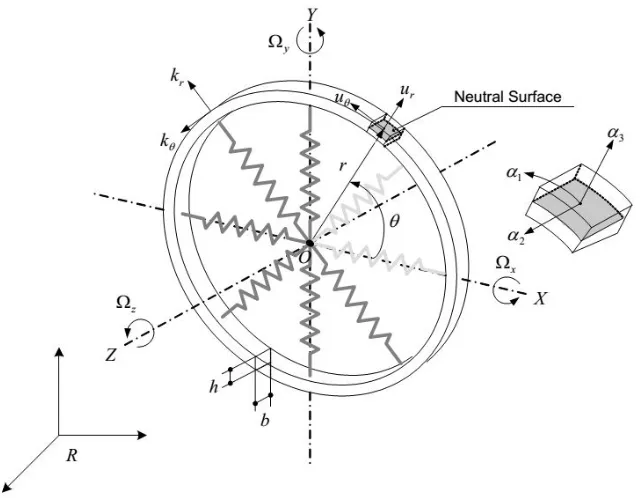
strain in mid-surface is zero and Galerkin’s procedure is employed to obtain the equations of motion in terms of suitable generalized coordinates. Figure 2.1 shows the geometry and parameters used in the present research.
Figure 2.1: Schematic of the rotating ring geometry. (Cho, 2005)
Chapter2. GoverningEquations 18
Rotational coordinates α1, α2 and α3 are used for locating the neutral surface elements and
ur anduθ represent the transverse and circumferential displacements, respectively. In order to
incorporate the stiffness of the ring into the model, eight radial springs are considered with the stiffness componentskr andkθ representing the radial and circumferential components,
re-spectively. Furthermore, the three components of the angular rate Ω are shown in the figure. However, the current analysis is focused on effects of angular rotation in theZ-axis direction and the other components are assumed to be zero. Due to the symmetry of the geometry, the ring exhibits different mode shapes with identical natural frequencies as shown in Figure 2.2, referred to as degenerate mode shapes. Energy transfer between these degenerate configura-tions due to angular rotation can be used in order to measure angular rate.
2.3
Governing Equations
For this particular mode, four generalized coordinates can be defined as shown in Figure 2.2, where the generalized coordinatesq1(t) andq2(t) represent the flexural displacements andq3(t)
andq4(t) represent circumferential displacements. It can be seen that the two configurations of
this mode are separated by 45◦ due to symmetry. In addition, the reversal of nodes and
anti-nodes in the two degenerate configurations has also been depicted in the figure. Furthermore, the derived equations of motion can be rewritten in terms of only the flexural modes by applying the amplitude ratios described by Huang and Soedel (1987),
q3 =−(1/n)q1 and q4 =(1/n)q2, (2.1)
The reduced discretized form of second order linear gyroscopic equations of motion for the ring using the flexural generalized coordinatesq= [q1 q2]T as:
Chapter2. GoverningEquations 20 M= 1 0 0 1+δm
(2.3) G=
0 −2Ωγ 2Ωγ 0
, (2.4) D=
2ζω01 0
0 2ζω02
, (2.5) K=
κ1+κ2Ω2 −Ω˙γ
˙
Ωγ κ1+κ2Ω2
, (2.6) F=
f1cosωt
0 . (2.7) where,
γ= bˆ˜ +n2aˆ˜ n(ˆ˜a+bˆ˜)
, κ1 =
ˆ˜
bcˆ˜−n2aˆ˜2 ρA(ˆ˜a+bˆ˜)
, κ2 =
n2(ˆ˜b+cˆ˜−4ˆ˜a)
ˆ˜
a+bˆ˜
− (2+n)(ˆ˜bcˆ˜−n
2aˆ˜)
(ˆ˜a+bˆ˜)2
!
,
ˆ˜
a=n2EI r4 +
EA
r2 , bˆ˜ = n 2EI
r4 +
EA r2
, cˆ˜ =n4EI r4 +
EA r2 .
The intermediate parameters ˜a, ˜b and ˜c are defined in Appendix A as the set of Equations (A.23).
The system matrix M is called the mass matrix. The effects of non-uniform distribution of mass along the circumference of the ring is incorporated in the mass matrix by employing the assumption that the mass of the ring is slightly higher, by the amountδmin the direction of the sensing coordinate. It may me noted that the stiffness matrix includes the centrifugal force term that depends on a factorκ2, which takes a negative value for the present system. Hence, overall
cou-pling term 2Ωγ, which is dependent on the input angular velocity. It is worth noting that owing to the gyroscopic as well as the centrifugal effects, the two undamped system natural frequen-ciesω01andω02vary with the input angular velocityΩ. However, at typical low input angular
velocities of about 2πrad/s, these two frequencies take nearly identical values (Asokanthan and Cho, 2006). The excitation frequency ω is usually chosen close to the system natural frequenciesω01andω02 which is discussed in detail in Section 2.4.
Keeping in mind that during the present research, the ring is excited only in one flexural mode, the force vector can be simplified to the form shown in Equation (2.7), where,
f1 =
2frbˆ˜
ρA(ˆ˜abˆ˜)
.
However, focusing on the system stability where the steady state response of the system is not of interest, the homogeneous form associated with Equation (2.2) in the absence of the excitation force f1is considered for the numerical analysis chapter of the thesis.
Moreover, the term ˙Ω can be neglected under the assumption of constant angular rate. On the other hand, this assumption is not practical in the presence of fluctuations in the angular rate. However, for the system under investigation, the contributions of the associated terms, ˙Ωγq1
and−Ω˙γq2 are negligible when compared to 2Ωγq˙1 and−2Ωγq˙2 at high angular rates where
instability becomes an issue. Therefore, it is sufficient to approximate ˙Ωγq1 = −Ω˙γq2 =0 for
the purpose of stability analysis. Also, for the case of uniform mass distribution of the ring, mass mismatchδm = 0. However, mass mismatch is taken into account for natural frequency computations, hence incorporating the effect of non-uniform distribution of mass in the system equations. Applying the assumed conditions, the governing equations of motion of a ring-based gyroscope take the form of a second order ordinary differential equation,
1 0 0 1 ¨ q+
2ζω01 −2Ωγ
2Ωγ 2ζω02
˙ q+
κ1+κ2Ω2 0
0 κ1+κ2Ω2
Chapter2. GoverningEquations 22
It is known that for a typical ring-based gyroscope operation, one of the second flexural modes is harmonically excited while the measurement of angular shift of this mode towards the cor-responding degenerate mode is employed in quantifying the angular rate. It may be noted that during the typical operation of a gyroscope an angular shift between 0◦ and 45◦ is realized as
discussed in Section 2.2 and earlier in Section 2.3. Hence, the coordinate q2 can be thought
of as being associated with the angular rate measurement while the coordinateq1can be
con-sidered to represent the excitation. For the purposes of numerical simulations, the geometric and material properties of the ring as shown in Table 2.1 have been used. In particular, these properties are employed to calculate the ring parametersγ,κ1 andκ2.
Property Value Density ρ=8800kg/m3
Young’s modulus E = 210×109N/m2
Mean radius r =500µm
Radial thickness h= 12.5µm
Axial thickness b=30µm
Table 2.1: Physical properties of the MEMS ring
2.4
Natural Frequency Variations
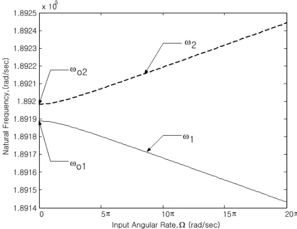
The natural frequencies of the two configurations of the second flexural mode depend on the mass mismatch factor as well as the angular rate of the ring. Using a micromachined ring-type sensor with isotropic material properties as described in Table 2.1, the variation of natural frequencies with angular rate can be obtained by Cho (2005) as depicted in Figure 2.3.
It can be seen that the natural frequencies of the two configurations remain the same in the absence of angular rate and mass anomalies. However, due to rotation of the ring about the
Figure 2.3: Variation of natural frequencies with angular rate with non-uniform mass assump-tion. (Cho, 2005)
the first flexural configuration decreasing while the second natural frequency is increased. Introducing mass mismatch to the system by settingδmas low as 0.01% results in the bifur-cation of the two natural frequencies in a stationary ring as shown in Figure 2.3. Similar to the ideal case, the first natural frequency is reduced with an increase in angular rate while the second natural frequency increases. Furthermore, increasing the mass mismatch consequently increases the bifurcation of natural frequencies.
2.5
Closure
Chapter2. GoverningEquations 24
Stochastic Model Incorporating
Uncertainty in Input Angular Rate
3.1
Introduction
Many physical phenomena can be modeled as random processes. When such a phenomenon appears in a dynamical system, the physical model takes the form of a Stochastic Differential Equation (SDE). SDEs appear in the modeling of certain phenomena due to the fluctuations which appear in, for example, the physical properties of a system and hence the coefficients of ordinary differential equations are no longer deterministic. Fluctuations may occur in many forms, a number of which are categorized based on the frequencies of the fluctuations.
In the present research, Gaussian white noise is selected to be fit as a wide bandwidth of frequencies is covered by this type of function. Advantages of using white noise include the ability to study the effects of a wider bandwidth of frequencies and perform more realistic simulations.
Chapter3. StochasticModel 26
3.2
Gaussian White Noise
White noise contains equal contributions from all visible frequency components. Whilst such processes seem to be physically impossible since the total energy of the signal would be in-finity, a white noise model of excitation is used very often and is found to be convenient in representing random processes. The reason is that any causal system only responds to a lim-ited range of excitation frequencies, therefore the components of the excitation which contain frequencies that are too high become irrelevant in predicting the system response. Ideal white noise is often used to simplify calculations and to obtain suitable orders of magnitude of the so-lution. Understanding the effect of white noise on the dynamic response of the system requires the basics of stochastic calculus which will be discussed in this chapter.
3.2.1
Stochastic Calculus
A stochastic process can be defined as any discrete or continuous process that is a collection of random variables associated with a deterministic parameter (Jekeli, 2001). A stochastic process
X can be mathematically defined as
(Xt,t ∈T)= (Xt(φ),t ∈T, φ ∈Φ),
defined on a space Φ, whereT is an arbitrary time interval. Keeping the definition in mind, a stochastic processW = (W(t),t ∈[0,∞]) is called a (standard) Brownian motion or Wiener process if the following conditions are satisfied (Mikosch, 1999; Kloeden and Platen, 1992):
• The process is continuous and starts at zero, i.e.,W(0)= 0.
• Expected value of the process is zero at any given time, i.e.,E[W(t)]= 0, and
distributionN(0,t−s).
White noise is defined as a wide-range stationary process ξ(t) with mean zero and constant spectral density functionS(ω)=S0, whereωrepresents any arbitrary frequency in the domain
[−∞,+∞]. The important properties of white noise can be summarized as:
• E[ξ(t)]=0, and
• E[W(t)W(t+τ)]=S0δ(t).
The name, ”white”, comes from the fact that the average power is distributed uniformly in fre-quency, similar to white light. Furthermore, considering a functionW(t), generating a Brow-nian motion with variance S0, it can be show that the first time derivative of W(t) is in fact
Gaussian white noise (Kloeden and Platen, 1992):
ξ(t)= dW
dt . (3.1)
This result is later on used in introducing noise to the geometrical system by generating a se-quence of random number based on a Brownian motion and using the numerical first derivative to simulate white noise.
3.3
Stochastic Fluctuation in Angular Rate
Chapter3. StochasticModel 28
reduction of order technique is employed. For this purpose four state variables are defined as:
q1 = x1, q˙1 = x2, q2 = x3, and ˙q2 = x4.
Substituting the defined variables x1 tox4into Equation (2.8) yields:
˙
x2+2ζω01x2−2Ωγx4+(κ1+κ2Ω2)x1 =0 (3.2)
(1+δm) ˙x4+2Ωγx2+2ζω02x4+(κ1+κ2Ω2)x3 =0 (3.3)
In order to represent the random fluctuation in the input angular velocity, these fluctuations are assumed to take the form of a white noise process. Understanding that the first time derivative of a Brownian motion process is Gaussian white noise, a Brownian motion function W(t) is employed to simulate the white noise (see e.g., Kloeden and Platen, 1992). Introducing the random fluctuation to a nominal input angular velocityΩ0, the input angular velocity is written
as:
Ω = Ω0+µ0ξ(t), (3.4)
where ξ(t) is white noise and µ0 is the noise intensity magnitude. Using Equation (3.4), the
centrifugal component of the equations of motion can be evaluated as:
Ω2= Ω2
0+2µ0Ω0ξ(t)+µ20ξ
2(t). (3.5)
The last term on the right hand side of Equation (3.5) is considered negligible due to its lower order of smallness, sinceµ0ξ(t) which represents fluctuations in angular rate is small relative to
the nominal angular rateΩ0and consequently µ20ξ2(t) 1. In order to better characterize the
fluctuation magnitude, a parameterµthat represents the noise intensity ratio is introduced as:
µ= µ0max(ξ(t))
max(Ω0)
Substituting Equations (3.4) and (3.5) in Equations (3.2) and (3.3) and multiplying the equa-tions bydtyields
dx2 =
2(Ω0+µ0
dW
dt )γx4−2ζω01x2−
κ1+κ2(Ω20+2µ0Ω0
dW dt )
2 x1
dt, (3.7)
dx4 =
1 1+δm
−2(Ω0+µ0
dW
dt )γx2−2ζω02x4−
κ1+κ2(Ω20+2µ0Ω0
dW dt )
2x 3
dt. (3.8) The equations for the four state variables can be obtained by simplifying the equations and neglecting the higher order terms:
dx1 = x2dt, (3.9)
dx2 =
2Ω0γx4−2ζω01x2−(κ1−κ2Ω20)x1
dt+2µ0γx4−2κ2µ0Ω0x1
dW, (3.10)
dx3 = x4dt, (3.11)
dx4 =
−2Ω0γx2−2ζω02x2−(κ1−κ2Ω20)x3
1+δm dt−
2µ0γx2−2κ2µ0Ω0x3
1+δm dW. (3.12)
Rewriting the equations in matrix form, a system of SDEs that represents the motion is obtained as: dx1 dx2 dx3 dx4 =
0 1 0 0
−κ1−κ2Ω2
0 −2ζω01 0 2Ω0γ
0 0 0 1
0 −2Ω0γ 1+δm
−κ1−κ2Ω2 0
1+δm
2ζω02
1+δm x1 x2 x3 x4 dt +
0 0 0 0
−2κ2µ0Ω0 0 0 2µ0γ
0 0 0 0
0 −2µ0γ 1+δm
−2κ2µ0Ω0
1+δm 0 x1 x2 x3 x4 dW, (3.13)
Chapter3. StochasticModel 30
the diffusion matrix,b[X(t)], with the state vectorX(t)= [x1 x2 x3 x4]T(see e.g., Higham,
2001; Kloeden and Platen, 1992; Higham and Kloeden, 2002). In the present numerical study, a smooth increase of the input angular rateΩ0from zero to 2πrad/s is employed for the purposes
of response predictions.
3.4
Itˆo-Taylor Expansion
It is known that an exact analytical solution does not exist for the stochastic differential equa-tions that represent the motion of a gyroscope. A numerical simulation of the system seems to be the most efficient method. For this purpose, a number of iterative approaches to integrate SDEs numerically have been developed in the recent past. The most widely-used ones are Euler-Maruyama, Euler-Heun, Milstein, derivative-free Milstein (Runge-Kutta approach), and Stochastic Runge-Kutta (see Schaffter, 2010). The higher-order Milstein scheme which takes advantage of the Itˆo-Taylor expansion for discretization of the SDE (Higham and Kloeden, 2002) is the most suitable for the present governing equations.
In an effort to describe this method, the Itˆo-Taylor expansion of the SDE for a scalar dependent variableX,
dX(t)= a[X(t)]dt+b[X(t)]dW(t) (3.14) is presented, wherea[X(t)] andb[X(t)], respectively, denote the drift and the diffusion terms while dW(t) represents the driving Wiener Process. Use of the Itˆo’s Lemma (Higham and Kloeden, 2002) leads to
d f[X(t)]= L0a[X(t)]dt+L1b[X(t)]dW(t), (3.15) where
L0 ≡ ∂
∂t +a
∂ ∂X +
1 2b
L1 ≡ b ∂
∂X,
and f(X[t]) is any function of X[t] with all functions evaluated at (t,x). The Itˆo formula can then be written in the form of the Itˆo stochastic integral equation:
f[X(t)]= f[X(t0)]+
Z t
t0
L0f[X(s)]ds+ Z t
t0
L1f[X(s)]dWs. (3.16)
Setting f(X)= Xand assuming thataandbdo not depend ontexplicitly, the equation becomes
X(t)= X(t0)+
Z t
t0
a[X(s)]ds+ Z t
t0
b[X(s)]dWs. (3.17)
Itˆo’s Lemma may be iterated to obtain constant integrands for the higher order terms. Choosing
f(X) = a[X(t)] and f(X)= b[X(t)] and applying Equation (3.16), the higher order coefficients are derived as
a[X(t)]= a[X(t0)]+
Z t
t0
L0a[X(s)]ds+ Z t
t0
L1a[X(s)]dWs, (3.18)
and
b[X(t)]= b[X(t0)]+
Z t
t0
L0b[X(s)]ds+ Z t
t0
L1b[X(s)]dWs. (3.19)
Substituting into Equation (3.17), yields
X(t)= X(t0)+
Z t
t0
(
a[X(t0)]+
Z s1
t0
L0a[X(s2)]ds2+
Z s1
t0
L1a[X(s2)]dW(s2)
) ds1 + Z t t0 (
b[X(t0)]+
Z s1
t0
L0b[X(s2)]ds2+
Z s1
t0
L1b[X(s2)]dW(s2)
)
dW(s1).
Chapter3. StochasticModel 32
Evaluation of the integrals follows:
X(t)=X(t0)+a[X(t0)]
Z t
t0
ds1+b[X(t0)]
Z t
t0
ds2
+Z t t0
Z s1
t0
L0a[X(t)]ds2ds1+
Z t
t0
Z s1
t0
L1a[X(s2)]dW(s2ds1
+Z t t0
Z s1
t0
L0b[X(s2)]ds2dW(s1)+
Z t
t0
Z s1
t0
L1b[X(s2)]dW(s2)dW(s1).
(3.21)
Substituting the functionsL0 andL1 as defined and carrying the integrals, the equation can be rewritten as
X(t)= X(t0)+a[X(t)]
Z t
t0
ds1+b[X(t)]
Z t
t0
dW(s1)
+b[X(t0)]b0[X(t0)]
Z t
t0
Z s1
t0
dW(s2)dW(s1)+O(δt3/2),
(3.22)
where O(δt3/2) represents terms that include δt3/2 or terms of higher order and b0 denotes derivative of functionbwith respect to variable X. The order of the terms are assessed with the the properties of Wiener process in mind, where E[dW2(t)] = dt and hence eachdW2 term is weighed similar in order as a first orderdtterm.
It should be noted that the double integral in Equation (3.22) is an Itˆo integral and therefore cannot be evaluated by classical calculus methods such as the conventional Reimann method. The double integral in Equation (3.22) can be evaluated using Itˆo integral rules as (Kloeden and Platen, 1992):
Z t
t0
Z s1
t0
dW(s2)dW(s1)=
1
2[W(t)−W(t0)]
2− 1
2(t−t0). (3.23) Substitution of the double integral in Equation (3.22) yields
X(t)= X(t0)+a[X(t)]
Z t
t0
ds1+b[X(t)]
Z t
t0
dW(s1)
+b[X(t0)]b0[X(t0)]{
1
2[W(t)−W(t0)]
2− 1
2(t−t0)}+O(δt
3/2
).
This equation forms the theoretical basis for both Euler and Milstein schemes (Higham and Kloeden, 2002). It may be noted that the Euler scheme is constructed using the first three terms of this expansion while incorporation of the fourth term yields the Milstein scheme. Considering the time interval [ti,ti+1], by choosing
t0 =ti, t =ti+1, ∆t =ti+1−ti, and∆Wi = W(ti+1)−W(ti),
the discretized form for the use of Milstein method is formulated as:
X(ti+1)= X(ti)+a[X(ti)]∆t+b[X(ti)]∆Wi+
1
2b[X(ti)]b
0
[X(ti)]
(∆Wi)2−∆t
, (3.25) where ∆W is a Wiener process with the properties E[W(t)] = 0 and E[W2(t)] = ∆t. For the purposes of numerical approximation,∆W can be generated using a uniformly distributed sequence of random numbers as (Kloeden and Platen, 1992):
∆W(ti)= N(0,1)∆ti (3.26)
Equation (3.25) when extended to multi-dimensional systems yields the component of the state vector employing Milstein scheme for numerical computations and takes the general form
Xu(t)i+1 = Xu(t)i +au[Xu(t)i]∆t+ m X
j=1
bu,j[Xu(t)i]∆W j i +
m X
j1,j2=1
Lj1bu,j2[Xu(t)
i]Ij1,j2, (3.27)
where the drift and diffusion terms, the driving Wiener process and the variables are written in vector form. In Equation (3.27),
Lj1 =
d X
k=1
bk,j1[Xu(t)
i]
∂
∂Xk, Ij1,j2 =
Z ti+1
ti
Z s1
ti
dWj1
s2dW
j2
s1,
b[X(ti)] is the diffusion coefficient matrix,dis the number of dimensions andmrepresents the
Chapter3. StochasticModel 34
The vector-based scheme presented in Equation (3.27), considering the system drift and diff u-sion coefficient matrices, is employed for the purposes of performing numerical computations to solve the system of equations that govern the gyroscope response. To this end, considering Equation (3.13) and settingdto 4 andmto 1 in Equation (3.27), the response takes the form:
Xu(ti+1)= Xu(ti)+au[Xu(ti)]∆t+bu,1[Xu(ti)]∆Wi +
4
X
k=1
1 2b
k,1[Xu
(ti)]
∂bu,1[X(ti)]
∂Xk
(∆Wi)2−∆t
, u= 1,2, . . . ,4.
(3.28)
The resulting four equations are employed in the prediction of gyroscope response.
Conforming to the goal of the present study, namely the stability investigation, free vibration of the gyroscope when subjected to an initial disturbance is examined.
3.5
Lyapunov Characteristic Exponent
The Lyapunov characteristic exponent for determining stability of dynamic systems was first introduced by Wolf et al. (1985). Lyapunov exponents are defined as the average rate of di-vergence or condi-vergence of nearby orbits in the n-dimensional phase space (Baker and Gollub, 1990). Any system with at least one positive Lyapunov exponent will inevitably become unpre-dictable, with the magnitude of the exponent reflecting on the time scale that system dynamics will diverge. Therefore, it is sufficient to only calculate the largest of the characteristic ex-ponents in order to determine system stability. In order to calculate Lyapunov exex-ponents, the long-term evolution of an infinitesimal n-sphere of initial conditions is observed as the spheres turn into n-ellipsoids. Theith one-dimensional Lyapunov exponent is then defined in terms of the ratio between the principal axes of the ellipsoid:
λi = lim t→∞
1
t pi(t) p0(t)
The method was further developed by Rosenstein et al. (1993) applied to small data sets with less computational effort. For the present work, the algorithm used was based on the method developed by Rosenstein et al. This method, as previously mentioned, requires reconstruction of the time response in phase space. For this purpose, the method of time delay as explained by Klikov´a and Raidl (2011), which is one of the most frequently used methods of phase space construction, was used. Using this algorithm, a parameter sweep was performed on noise intensity for different values of damping ratios. The details of the computer code used for this purpose can be found in Appendix B.
3.6
Closure
Chapter 4
Stability Analysis Using Numerical
Methods
4.1
Introduction
For the purposes of studying the stability of the gyroscope, time response for the free vibration of the system is examined, when the system is subjected to suitable initial conditions. Sim-ulations performed are based on an assumption that an initial displacement of 10−5m being exerted on the driving coordinate, q1, while stochastic fluctuations in input angular rate are
applied as described in Equation (3.4). The sensing coordinate q2 is then quantified for the
purposes of characterizing the gyroscope response.
Initially, the predicted responses using the higher-order Milstein scheme are compared with the results obtained using the simpler Euler scheme in order to assess the validity of the developed Milstein algorithm and also investigate the benefits of using a higher-order scheme. Moreover, the Largest Lyapunov Exponents of the predicted responses are evaluated in order to study the stability of the system. Finally, the higher-order Milstein scheme is used in order to find the stability threshold of the system under stochastic fluctuation and considering different damping
ratio values. The developed Matlab code is discussed in detail in Appendix B. The hardware used for numerical calculations consisted of a Windows 7 PC with an AMD Phenomtm Quad Core processor clocked at 2.2 GHz and 8GB of memory.
4.2
Numerical Predictions
In order to ascertain the accuracy of the developed model, the convergence of the simulation algorithm is tested with four different damping ratio values, namely 0.03, 0.05, 0.09 and 0.13. Numerical convergence is reached in 150000 or more time steps for a duration of 0.009 seconds of simulation time and the number of time steps is considered adequate for the remainder of the study.
The vector-based higher-order Milstein scheme has been chosen for this study instead of the
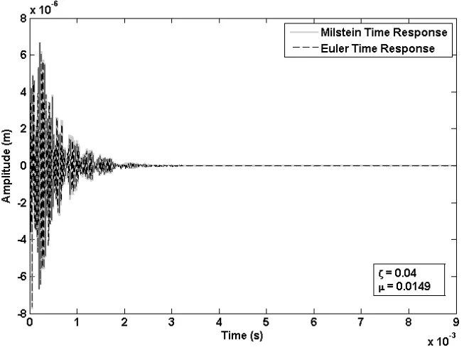
Figure 4.1: Example of stable time response.
Chapter4. StabilityAnalysisUsingNumericalMethods 38
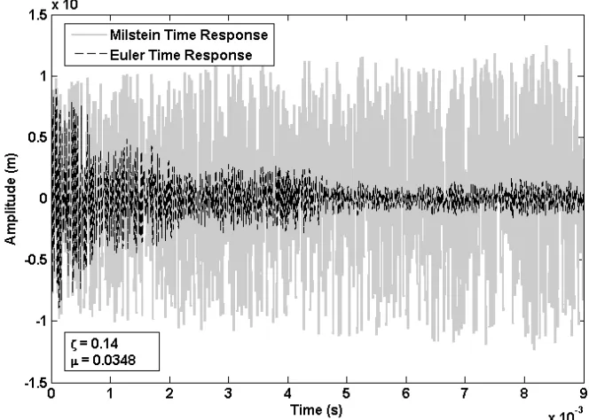
the numerical simulations by employing a higher-order scheme. System time responses gener-ated by the two methods were compared for the purposes of verifying the response predictions. Figures 4.1 to 4.3 show the responses of the gyroscope under different fluctuation magnitudes and displaying both stable and unstable behavior of the system. The Wiener process is numer-ically simulated using the random number generation function in MATLAB and employing the method discussed in Equation (3.26). The details of the developed MATLAB code used for generation of the Wiener process are available in Appendix B.2. Maximum relative noise intensity, as defined in Equation (3.6) has been used as a magnitude measure for representing environment fluctuation. Figure 4.1 shows the response of the system for a damping ratio of 0.04 and maximum relative noise intensity measureµ= 0.0149.
It can be seen that with sufficient damping, the system is observed to remain stable. However, as shown in Figure 4.2, as noise intensity is increased to a sufficiently high value to cause noticeable disturbance in the system, yet low enough to be damped, the system shows oscilla-tory motion until complete decay. It may be noted that a certain threshold intensity measure for each damping ratio is associated with transition to instability and this measure can be computed using the time responses.
Figure 4.2: Example of marginally stable time response.
Chapter4. StabilityAnalysisUsingNumericalMethods 40
Figure 4.4: Under-prediction of results by Euler scheme in a marginally stable case.
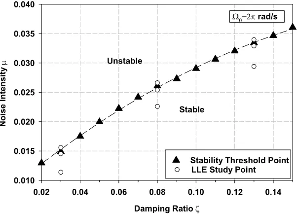
For the purposes of confirming that the results from Milstein and Euler schemes are com-patible, and also for studying the error introduced by neglecting higher-order terms in Euler scheme, a number of points have been chosen for the LLE study. Three highly stable points that correspond to damping ratios of 0.03, 0.08 and 0.13 and the respective maximum relative noise intensity values of 0.0114, 0.0225 and 0.0294 as displayed in Figure 4.6 have been cho-sen. LLE values evaluated at these points resulted in the same sign, in this case being negative confirming that the system is stable under such conditions. However, LLE values predicted by Eulers scheme have been found to be lower than those predicted by Milstein Scheme by 3.8 to 8.5 percent. Further, comparison of the time responses predicted by these two schemes reveals that the Euler scheme tend to under-predict the response for the present gyroscopic system. Hence, it may be concluded that contribution from the higher-order terms could be significant and the use of Milstein scheme is beneficial in some cases. However, for the purposes of pre-dicting the response of this class of gyroscopes Euler scheme offers lower computation time
Chapter4. StabilityAnalysisUsingNumericalMethods 42
and resource requirements. The details of the LLE calculations are summarized in Table 4.1. It should be noted that the difference percentage is calculated by considering the difference between the LLE values obtained using Milstein and Euler schemes divided by the LLE value obtained using Euler scheme.
Damping Ratioζ Raw noise intensityµ0 Milstein Euler Relative Difference
0.03 65 -1.31E+08 -1.35E+08 -3.8% 83 -1.72E+07 -2.28E+07 -24.3% 87 2.33E+07 2.20E+07 5.87% 0.08 129 -2.57E+08 -2.77E+08 -7.07%
147 -1.22E+07 -3.39E+07 -64% 152 6.36E+07 5.67E+07 12.1% 0.13 168 -4.05E+08 -4.43E+08 -8.5% 188 -5.93E+07 -9.80E+07 -39.5% 194 3.73E+07 4.11E+07 -9.04% Table 4.1: Summary of LLE values for predicted time responses.
In order to further confirm that the two schemes predict approximately compatible instability thresholds for the system, six marginal points as shown in Figure 4.6 have been chosen for analysis. Three points slightly above the threshold point within the unstable region and three points slightly below within the stable region have been chosen. The LLE analysis reveals that both schemes predict the LLE value with the same sign and therefore predicting stability and instability regions correctly.
4.3
Parametric Study
Damping Ratio
0.02 0.04 0.06 0.08 0.10 0.12 0.14
Noise I
ntensity
0.010 0.015 0.020 0.025 0.030 0.035 0.040
Stable
rad/s
Stability Threshold Point LLE Study Point
Unstable
Figure 4.6: Stability boundary in theµ-ζspace (Ω =2πrad/s).
Chapter4. StabilityAnalysisUsingNumericalMethods 44
velocity, affecting overall system stiffness. Further, it has been found that moderate changes in mass mismatch do not affect the noise threshold. However, unrealistic mass mismatch values close to 10 percent cause a reduction in the second natural frequency and as a consequence appear to contribute to a reduction in the noise threshold. It is worth noting that such values for mass mismatch and angular velocity are not of practical significance under typical gyroscope operating conditions. Variation of system natural frequencies with mass mismatch can be seen in Table 4.3. It should also be noted that increasing the mismatch only results in the reduction of the first natural frequency while the second natural frequency of the system is unaffected by the mismatch at a constant angular rate.
Ω0(rad/s) ω01(rad/s) ω02(rad/s) Change Relative to Stationary Ring
0 1.9864×10⁵ 1.9865×10⁵
-2π 1.9864×10⁵ 1.9865×10⁵ 0 % 10π 1.9862×10⁵ 1.9867×10⁵ 0.01%
Table 4.2: Variation of system natural frequencies with input angular rate.
δm ω01(rad/s) ω02 (rad/s) Change Relative to Stationary Ring
0 1.9864×10⁵ 1.9865×10⁵ -10−4 1.9864×10⁵ 1.9865×10⁵ 0 %
10−3 1.9855×10⁵ 1.9865×10⁵ 0.04%
10−2 1.9766×10⁵ 1.9865×10⁵ 0.49% 10−1 1.8940×10⁵ 1.9865×10⁵ 4.65%
Table 4.3: Variation of system natural frequencies with mass mismatch.
4.4
Closure
Chapter 5
Experimental Results
5.1
Introduction
In this chapter, the variations in natural frequency due to angular rate as well as manufacturing imperfections are studied by employing an experimental setup. The secondary objective of the conducted experiments is to demonstrate the phenomena that might not be otherwise easily investigated through a MEMS sensor such as nonlinear behavior that arises due to the smallness of natural frequency of a macro-scale ring-type angular sensor. Phenomena such as variations in system natural frequency due to the presence of input angular rate and decreased uniform distribution of mass as well as the effect of fluctuations in angular rate on system behavior are studied.
The experiments that are conducted in the present chapter are merely a means of observation of the expected behavior and not reproduction of the numerical results presented in Chapter 4. Further validation of results against theoretical data is not feasible due to the differences in the geometries used in the analysis. The predicted numerical results are obtained using the properties of a MEMS-scale geometry while the experimental data involves a macro-scale ring. This results in a significant difference in system natural frequency and therefore the input
angular rate being relatively higher than a MEMS-scale ring. Furthermore, the vibrations in the experimental setup are of high amplitude making contact-less sensing feasible, detection of the vibrations and natural frequencies possible with the naked eye and thus, resulting in increased non-linearity of the system.
Similar to Chapter 4, an experiment has been designed in order to study the effects of fluctua-tions in input angular rate on system behavior. However, due to the limitafluctua-tions of the physical system, it is not yet possible to reproduce the obtained numerical results. Therefore, a prelimi-nary experiment has been designed in order to reveal the effects of input fluctuation, the results of which can be used in future experiments on quantifying the effects of stochastic fluctuations in input angular rate.
5.2
Experimental Setup
The experimental setup consists of a long suspended C1095 blue-tempered cylindrical McMaster-Carr Supply Company steel shell with the properties summarized in Table 5.1. The shell is made by joining the two sides of a steel plate using spot welding and therefore natural vari-ations in mass mismatch as well as damping and stiffness are expected. However, it should be noted that the analytical and numerical studies in the present thesis are performed with a micro-scale ring in mind. In order to overcome the complexities of manufacturing a MEMS ring as well as associated problems with excitation and sensing methods, the constructed long macro-scale cylinder was considered for the experimental analysis instead, due to the similar-ities between dynamic characteristics of a non-rotating ring structure and a non-rotating long cylindrical structure (Cho, 2009).