DOA Estimation with Sparse Array Under Unknown Mutual Coupling

DOA Estimation with Sparse Array under Unknown

Mutual Coupling

Sheng Liu, Jing Zhao*, and Zhengguo Xiao

Abstract—In this paper, we propose a direction-of-arrival (DOA) estimation algorithm under unknown mutual coupling with a sparse linear array (SLA). We employ an SLA composed of two uniform linear arrays (ULA), and the element spacing of one of the subarrays is large enough to neglect the effect of the mutual coupling (MC). The fourth-order-cumulants (FOCs) of the received data from partial elements of the first subarray and all elements of the second subarray are exploited to construct a high-order FOC matrix. Then, the DOAs of incident signals are estimated by dealing with this high-order matrix. The array aperture is extended greatly due to the sparse structure. Hence, the proposed method shows much better performance than some classical blind DOA estimation methods in accuracy and resolution. We also propose some simulation results to prove the effectiveness of our method.

1. INTRODUCTION

Antennas play a very important role in wireless communication systems. The design method for smart antennas [1] and planar array [2] has been presented and shown improved performance in some aspects. Direction-of-arrival (DOA) estimation of incident signals is a momentous embranchment of array signal processing, and it also has received widespread concern in wireless communication [3]. Many classical DOA estimation techniques such as subspace-based methods [4–6], sparse reconstruction algorithms [7, 8] and support vector classification-based algorithm [9] were proposed by scholars in succession. However, most of these algorithms are conditional on that mutual coupling (MC) between sensors is ignored or known. In fact, MC exists unavoidably, particularly between the elements with small spacing, and it can affect the structure of array manifold. So the methods [4–9] are difficult to achieve satisfactory estimation performance in practice

Recently, in order to eliminate the effect of MC, many calibration algorithms [10–18] have been presented. Iterative method [10–12] is a commonly used technology to estimate MC coefficients (MCCs), but this method cannot estimate the DOA directly. The authors in [13] constructed a cost function, where the MCCs were separated from this cost function. Then, the directions of incident signals can be estimated by minimizing this cost function under unknown MCC (For convenience, we called this method as MCCS method). Though this method can eliminate the calculation burden by estimating the MCC, the performance of this method will decline sharply under low SNR or small angle interval environment. In [15], only the middle subarray (MS) of a ULA is utilized, and the DOA can be estimated without knowing the MCC (For convenience, we call this method as MS method). This technique was also applied to an L-shaped array in [16] and coherent signals in [17]. However, an obvious shortcoming of MS method is aperture loss. Moreover, the performances of these methods degrade when the incident direction is close to 90◦. In [18], an MS method based on FOC (FOC-MS) was proposed, but the computational complexity of this algorithm is very large. Some sparse

Received 17 August 2017, Accepted 21 September 2017, Scheduled 4 October 2017 * Corresponding author: Jing Zhao ([email protected]).

arrays [19, 20] with reduced mutual coupling have been proposed, but these arrays cannot contribute to eliminating mutual coupling.

In this paper, we employ two different uniform linear arrays (ULAs) to constitute a sparse linear array, which can be seen as a special two-level nested array [21–23]. The element spacing of the second ULA is far larger than the half-wavelength of incident signals. Hence, the effect of MC on this subarray can be neglected, and the array aperture is extended greatly. The received data from the second ULA and middle subarray of the first ULA are used to reconstruct an extended FOC matrix. Then, we can get the estimation of DOA by the traditional subspace-based algorithm [4]. The proposed method has much higher accuracy and resolution than the MCCS, MS and FOC-MS methods. It is worthy to mention that the computational complexity of the proposed algorithm is lower than the FOC-MS method.

2. DATA MODEL

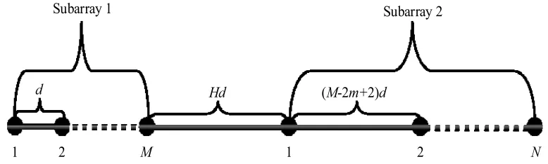
Assume that MC only exists between the elements with space distance less than m₂λ, where λ is the wavelength of incoming signals. We consider a nonuniform linear array consisting of two uniform linear arrays, and the array architecture is shown in Fig. 1. d= λ₂ is the distance between adjacent elements of the first subarray. The element spacing of the second subarray is (M−2m+ 2)d. Hdis the distance between the two subarrays, where (M−2m+ 2) ≥m andH ≥m. Suppose that the first sensor of the first subarray is the reference element. Consider K narrowband incoherent and non-Gaussian signals

s1(t), . . . , sK(t) coming from the directions θ = [θ1, . . . , θK]. Assume that M is an odd number and

J =M −2m+ 2 and L= M−2₂m+1.

Let x1(t) = [x1,1(t), . . . , x1,M(t)]T ∈ CM×1, x2(t) = [x2,1(t), . . . , x2,2(t), x2,N(t)]T ∈ CN×1 be the

received vectors of two subarrays, and the vectors can be expressed as

x1(t) = CA1(θ)s(t) +n1(t) (1)

x2(t) = A2(θ)s(t) +n2(t) (2)

where s(t) = [s1(t), . . . , sK(t)]T ∈ CK×1 is the non-Gaussian signal vector; A1(θ) =

[a1(θ1), . . . , a1(θK)]∈CM×K,A2(θ) = [a2(θ1), . . . , a2(θK)]∈CN×K,a1(θk) = [1, . . . , e−jπ(M−1) sinθk]T ∈

CM×1, a2(θk) = [e−jπ(M−1+H) sinθk, e−jπ(M−1+H+J) sinθk, . . . , e−jπ(M−1+H+(N−1)J) sinθk]T ∈ CN×1;

n1(t) = [n1,1(t), . . . , n1,M(t)]T ∈ CM×1 and n2(t) = [n2,1(t), . . . , n2,N(t)]T ∈ CN×1 are additive white

Gaussian noise vectors;C is the MC matrix (MCM) with the structure as [13, 15, 17]

C= ⎡ ⎢ ⎢ ⎢ ⎢ ⎢ ⎢ ⎢ ⎢ ⎢ ⎢ ⎢ ⎢ ⎣

c1 . . . cm 0 0 . . . 0

..

. . . . ... ... ... ... ...

cm . . . c1 . . . cm . .. 0

0 . . . ... ... ... ... 0 0 . . . cm . . . c1 . . . cm

..

. . . . ... ... ... ... ... 0 . . . 0 0 cm . . . c1

⎤ ⎥ ⎥ ⎥ ⎥ ⎥ ⎥ ⎥ ⎥ ⎥ ⎥ ⎥ ⎥ ⎦ (3)

LetJ = [0(2L+1)×(m−1), I2L+1,0(2L+1)×(M−2L−m)] with M−2₂m+1 =L as [17], then we have

˜

x1(t) = Jx1(t)

= ˜CA1(θ)˜s(t) + ˜Cn1(t)

= ˜A1(θ)˜s(t) + ˜n1(t)

where ˜A1(θ) = [˜a1(θ1), . . . ,˜a1(θK)] ∈ C(2L+1)×K, ˜a1(θk) = [ejπLsinθk, . . . ,1, . . . , e−jπLsinθk]T ∈

M N

d _{Hd (M-2m+2)d}

Subarray 1 _{Subarray 2}

1 2 1 2

Figure 1. Framework of sparse linear array.

c1e−jπ(L+m−1) sinθk+. . .+cme−jπ(L+2m−2) sinθk, k = 1,2, . . . , K; ˜x1(t) = [˜x1,1(t), . . . ,x˜1,J(t)]T ∈CJ×1,

˜

n1(t) = [˜n1,1(t), . . . ,n˜1,J(t)]T ∈CJ×1, and ˜C can be expressed as

˜

C= ⎡

⎣ cm . . . c1 . . . cm . . . 0 ..

. . .. ... ... ... ... ... 0 . . . cm . . . c1 . . . cm

⎤

⎦ (4)

3. ALGORITHM DESCRIPTION

3.1. The Reconstruction of FOC Matrix

In this subsection, a high-order FOC matrix R∈CJN×JN is constituted by the FOC of received data. LetRuv=cum{x2u₂,x˜∗_1(J−u1+1), x∗2v₂,x˜1(J−v1+1)}be the element of the uth row and vth column ofR,

and u1, u2, v1, v2 are determined uniquely byu, v according to

u=u1+u2J

v=v1+v2J

(5)

where 1≤u1, v1 ≤J, 0≤u2, v2 ≤N −1.

From Eq. (5), we have

Ruv = cum x2u2,x˜∗1(J−u1+1), x∗2v₂,x˜1(J−v1+1)

= cum

_K

k=1

e−jπ[M−1+H+(u2−1)J] sinθ_k

sk+n2,u2(t),

K

k=1

ejπ(J−u1−L) sinθ_k˜

s∗_k+ ˜n∗1,u1(t),

K

k=1

ejπ[M−1+H+(v2−1)J] sinθk_s∗

k+n∗2,v2(t),

K

k=1

e−jπ(J−v1−L) sinθk_{˜sk+ ˜n1,v} 1(t)

(6)

It is easy to know that

cum{sk,˜s∗k, s∗k,˜sk} = cum{sk(t), c∗(θk)s∗k(t), s∗k, c(θk)sk(t)}

Because the FOC of Gaussian noise is 0, Eq. (6) can be rewritten as

Ruv = K

k=1

pke−jπ(u−v) sinθk

+cum{n2,u2(t),n˜∗1,u₁(t), n2∗,v₂(t),n˜1,v1(t)}

=

K

k=1

pke−jπ(u−v) sinθk (8)

wherepk=|c(θk)|2cum{sk,s˜∗_k, s∗_k,s˜k}

According to Eq. (8), we have

R=BSBH (9)

where S = diag{p1, p2, . . . , pK}; B(θ) = [b(θ1), b(θ2), . . . , b(θK)] ∈ CJN×K; b(θk) =

[1, . . . , e−jπ(JN−1) sinθk_]T ∈_CJN×1_{,k= 1,2, . . . , K.}

EVD of matrixR yields

R=EsDsE_sH +EnDnE_nH (10) where Ds = diag{λ1, . . . , λK}, and λ1, . . . , λK are the K largest eigenvalues. At last, we can get the

estimation of θby MUSIC [4].

3.2. Complexity Analysis

In this subsection, we only compare the computational complexity of the proposed method with FOC-MS method [18]. The major computational complexity of the proposed algorithm isO{9(N J)2T+ (N J)3+

P(N J)2(N J−K)}, whereJ =M−2m+ 2 andP is the scanning times. For the FOC-MS method [18], the major computational complexity is O{9J14T+J16+P J14(J12−K)}, where J1 =M +N −2m+ 2.

Obviously, the complexity of proposed method is lower than FOC-MS method. In addition, the proposed method and FOC-MS method have higher computational complexity than the second order statistics-based methods [13, 15].

Figure 2. Space spectrum of four algorithms ([θ1, θ2, θ3] = [20◦,40◦,60◦]).

4. SIMULATION RESULTS

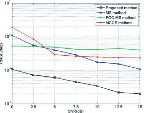
In this section, we perform several simulations to assess the performance of presented method, MCCS method [13], MS method [15] and FOC-MS method [18]. We assume that M = 9, N = 5, H = 5. Meanwhile, we employ a 14-element ULA with half-wavelength element spacing for the MCCS method, MS method and FOC-MS method. Let m = 3, c1 = 1, c2 = 0.9 + 0.4i, c3 = 0.5−0.3i, and scanning

intervalω= 0.1◦ in the simulations below. Define the root mean square error (RMSE) as

RM SE =

1

100K

100

j=1 K

k=1

(ˆθkj−θk)2 (11)

where ˆθkj is the estimation ofθk in thejth Monte Carlo trial.

Firstly, some simulations for comparison of resolution are carried out. Figs. 2, 3, 4, 5 show the space spectrums of the four methods under four different scenarios. Keep the number of snapshots at 200 and the SNR at 10 dB. Assume that four groups directions of three incident signals are [θ1, θ2, θ3] =

[20◦,40◦,60◦], [θ1, θ2, θ3] = [25◦,40◦,55◦], [θ1, θ2, θ3] = [30◦,40◦,50◦] and [θ1, θ2, θ3] = [35◦,40◦,45◦],

respectively. The comparison result in Fig. 2 indicates that the three directions with 20◦ angle interval can be discriminated clearly by the four algorithms. The discrimination of MCCS method is beginning to degrade as the angle interval narrows from 15◦to 5◦, which can be seen from Figs. 3, 4, 5. In addition, from Fig. 4, we can see that the DOAs of these signals can be distinguished reluctantly by MCCS and MS when the angle interval is 10◦. But when the angle interval is 5◦, only our method can discriminate the three directions, which is reflected from Fig. 5. Considering the comparison results from the four figures, we can say that our algorithm has higher resolution than the other three algorithms.

Figure 4. Space spectrum of four algorithms ([θ1, θ2, θ3] = [30◦,40◦,50◦]).

Figure 5. Space spectrum of four algorithms ([θ1, θ2, θ3] = [35◦,40◦,45]).

Figure 6. RMSE versus SNR. Figure 7. RMSE versus snapshots.

5. CONCLUSIONS

In this paper, a DOA estimation algorithm in the case of MC is addressed. Large interval ULA and small-interval ULA are used simultaneously to reduce the effect of MC. Because of the extension of array aperture, the estimation performance is better than many traditional blind DOA estimation algorithms in accuracy and resolution. From the simulation results in Section 4, we can know that the proposed method can get satisfactory estimation precision for different directions even if under a low SNR environment. Moreover, compared with the FOC-based algorithm, our algorithm not only has higher accuracy and resolution but also has lower computation complexity.

ACKNOWLEDGMENT

The authors would like to thank the editors and anonymous referees for their comments and suggestions that help us to improve the quality of this paper.

REFERENCES

1. Viani, F., L. Lizzi, M. Donelli, D. Pregnolato, G. Oliveri, and A. Massa, “Exploitation of parasitic smart antennas in wireless sensor networks,” Journal of Electromagnetic Waves and Applications, Vol. 24, No. 7, 993–1003, 2010.

2. Donelli, M. and P. Febvre, “An inexpensive reconfigurable planar array for Wi-Fi applications,”

Progress In Electromagnetics Research C, Vol. 28, 71–81, 2012.

3. Albagory, Y. A., “Performance of 2-d DOA estimation for stratospheric platforms communications,”

Progress In Electromagnetics Research M, Vol. 36, 109–116, 2014.

4. Schmidt, R. O., “Multiple emitter location and signal parameter estimation,” IEEE Transactions on Antennas &Propagation, Vol. 34, No. 3, 276–280, 1986.

5. Wen, F., Q. Wan, R. Fan, and H. Wei, “Improved music algorithm for multiple noncoherent subarrays,” IEEE Signal Processing Letters, Vol. 21, No. 5, 527–530, 2014.

6. Roy, R. and T. Kailath, “Esprit-estimation of signal parameters via rotational invariance techniques,” IEEE Transactions on Acoustics Speech & Signal Processing, Vol. 37, No. 7, 984– 995, 1989.

8. Yang, Z., L. Xie, and C. Zhang, “Off-grid direction of arrival estimation using sparse Bayesian inference,”IEEE Transactions on Signal Processing, Vol. 61, No. 1, 38–43, 2013.

9. Massa, A., M. Donelli, F. Viani, and P. Rocca, “An innovative multiresolution approach for DOA estimation based on a support vector classification,” IEEE Transactions on Antennas and Propagation, Vol. 57, No. 8, 2279–2292, 2009.

10. Friedlander, B. and A. J. Weiss, “Direction finding in the presence of mutual coupling,” IEEE Transactions on Antennas and Propagation, Vol. 39, No. 3, 273–284, 1991.

11. Bao, Q., C. C. Ko, and W. Zhi, “DOA estimation under unknown mutual coupling and multipath,”

IEEE Transactions on Aerospace & Electronic Systems, Vol. 41, No. 2, 565–573, 2005.

12. Cao, S., D. Xu, X. Xu, and Z. Ye, “DOA estimation for noncircular signals in the presence of mutual coupling,” Signal Processing, Vol. 105, No. 12, 12–16, 2014.

13. Wang, B. H., Y. L. Wang, H. Chen, and X. Chen, “Robust DOA estimation with uniform linear array under mutual coupling and selfcorrection of mutual coupling,” Science China Ser. E Technological Science, Vol. 34, No. 2, 229–240, 2004.

14. Li, H. B., Y. D. Guo, J. Gong, and J. Jiang, “Mutual coupling self-calibration algorithm for uniform linear array based on ESPRIT,”IEEE International Conference on Consumer Electronics, Communications and Networks, 3323–3326, 2012.

15. Ye, Z. and C. Liu, “On the resiliency of music direction finding against antenna sensor coupling,”

IEEE Transactions on Antennas & Propagation, Vol. 56, No. 2, 371–380, 2009.

16. Liang, J., X. Zeng, W. Wang, and H. Chen, “L-shaped array-based elevation and azimuth direction finding in the presence of mutual coupling,”Signal Processing, Vol. 91, No. 5, 1319–1328, 2011. 17. Mao, W. P., G. L. Li, X. Xie, and Q. Z. Yu, “DOA estimation of coherent signals based on direct

data domain under unknown mutual coupling,” IEEE Antennas Wireless Propag. Lett., Vol. 13, 1523–1528, 2014.

18. Liu, C., Z. Ye, and Y. Zhang, “DOA estimation based on fourth-order cumulants with unknown mutual coupling,” Signal Processing, Vol. 89, No. 9, 1839–1843, 2009.

19. Liu, C. L. and P. P. Vaidyanathan, “Super nested arrays: Linear sparse arrays with reduced mutual coupling — Part I: Fundamentals,”IEEE Transactions on Signal Processing, Vol. 64, No. 15, 3997– 4012, 2016.

20. Liu, C. L. and P. P. Vaidyanathan, “Super nested arrays: Linear sparse arrays with reduced mutual coupling — Part II: High-order extensions,” IEEE Transactions on Signal Processing, Vol. 64, No. 16, 4203–4217, 2016.

21. Pal, P. and P. P. Vaidyanathan, “Nested arrays: A novel approach to array processing with enhanced degrees of freedom,”IEEE Transactions on Signal Processing, Vol. 58, No. 8, 4167–4181, 2010.

22. Liu, S., L. S. Yang, D. Li, and H. L. Cao, “Subspace extension algorithm for 2D DOA estimation with L-shaped sparse array,” Multidimensional Systems & Signal Processing, Vol. 28, No. 1, 315– 327, 2017.