Abstract—This paper presents a microwave imaging for brain tumour detection utilizing Forward-Backward Time-Stepping (FBTS) inverse scattering technique. This technique is applied to solve electromagnetic scattered signals. It is proven that this technique is able to detect the presence of tumour in the breast. The application is now extended to brain imaging. Two types of results are presented in this paper; FBTS and FBTS integrated with image segmentation as a pre-processing step to form a focusing reconstruction. The results show that the latter technique has improved the reconstructions compared to the primary technique. Integration of the image segmentation step helps to reduce the variation of the estimated dielectric properties of the head tissues. It is also found that the optimal frequency used for microwave brain imaging is at 2 GHz and able to detect a tumour as small as 5 mm in diameter. The numerical simulations show that the integration of image segmentation with FBTS has the potential to provide useful quantitative information on the head internal composition.
1. INTRODUCTION
Brain tumour is a highly-reported malignancy around the world for its deadly effect if left untreated. According to Brain Tumour Research Report [1], brain tumour kills more children and adults under the age of 40 than any other cancers. A primary brain tumour is a cluster of an abnormal tissue that originates from the brain tissue, and secondary brain tumour originates from other cancer cells inside the body and metastases to the brain through blood stream. Meningioma and glioma are the most common types of brain tumour and account for approximately 61% of the primary tumour, and the latter is highly malignant [2]. They commonly grow at the cerebellum hemisphere of the brain. It is important to determine if the tumour is able to metastasize in order for radio-surgical management procedure to be arranged to control the tumour from spreading. The tumour size plays an important role to ensure the successful rate of the local control. As reported in [3], 87% success local control rate can be achieved if the tumour size is less than 1 cm in diameter; otherwise, the percentage will be reduced from 50% to 24%. Thus, early detection of the tumour is crucial to ensure that the tumour can be controlled from spreading to other parts of the brain or the body.
Microwave imaging is a well-established technique among researchers and industries and is employed to build a low cost and portable diagnostic machine [4–6]. Near-field electromagnetic imaging (EMI) using energy in radio and microwave frequency ranges is an attractive topic particularly in biomedical imaging [7, 8]. One of the key elements in any microwave imaging system is the inversion technique used to determine the location, shape and electrical properties of an unknown embedded object. Numerous
Received 6 July 2017, Accepted 17 September 2017, Scheduled 24 October 2017 * Corresponding author: Kismet Anak Hong Ping ([email protected]).
1 Applied Electromagnetic Research Group, Faculty of Engineering, Universiti Malaysia Sarawak, Kota Samarahan, Sarawak 94300,
researches have been carried out on biomedical imaging for breast cancer detection by using inverse scattering technique and come out with successful results but none being applied to head imaging [9– 11]. Due to the success in detecting the breast cancer, inverse scattering technique demonstrated a high potential in detecting brain tumour. Microwave imaging for head is challenging because of complex layered tissues in the brain. This paper is a pilot study, presenting results and discussion on head imaging for brain tumour detection by using inverse scattering technique.
A two-dimensional (2D) Forward-Backward Time-Stepping (FBTS) inverse scattering technique has been applied to the breast and demonstrated good results in detecting tumours in the breast [12–15]. Therefore, the focus of this paper is on a brain tumour detection utilizing inverse scattering technique in 2D head model. A homogenous head model of an MRI in 3D (.mnc format) is obtained from [16, 17]. A slice from the head model is selected to get the 2D transverse plane view, and this slice is then used as an object under test (OUT). For numerical analysis purposes, we consider 4 significant tissue types: skin, skull, grey matter (GM) and white matter (WM). The head model contains dielectric properties with high contrast between the skin and skull, and low contrast between GM and WM. This paper demonstrates the ability of the inverse scattering technique to detect an embedded tumour of different sizes in WM region. Safety was taken into account for microwave imaging even though electromagnetic wave is non-ionizing wave and has a certain impact on biological beings as it can increase the temperature at the area of incident wave. However, limiting the frequency to less than 6 GHz for a certain amount of time of exposure on tissues at a distance of 200 mm and below helps to prevent an adverse thermal effect [18, 19]. Therefore, a near-field EMI is used for this research.
2. METHOD
2.1. Forward-Backward Time-Stepping
Forward-Backward Time-Stepping (FBTS) is a technique to solve inverse scattering problem in time domain. Scattered signal transmitted from an antenna through an object is collected by receivers and solved by using FBTS algorithm to get the object’s information. The aim of using FBTS to solve electromagnetic inverse scattering is to determine the shape, location and electrical properties of the object [20–22]. A cost functional formula is used to help in minimizing number of iterations of the FBTS reconstruction:
F(p) = cT 0 M m=1 N n=1
Kmn(t)Vm(p;rn,t)−V˜m(rn,t)|2d(ct) (1)
where p is a set of variable dielectric values (permittivity and conductivity); c is the speed of light; T is the measurement time period,tis the time,m and nrepresent transmitting and receiving antennas, respectively; Kmn(t) is a weighting function of non-negative that holds a value of zero when t = T;
˜
Vm(rnt) are the measured electromagnetic field in time domain at positionrn antenna due to pulse of mtransmitter, whereas Vm(rnt) is the calculated electromagnetic field for a set of material parameters. Since the gradient method for cost functional minimization as in Equation (1) is applied, the gradient of the error functional with respect to permittivity and conductivity is necessary given by [23];
g(r) = (gε(r), gσ(r))t (2)
where,
gε = cT 0 M m=1 3 i=1
wmi(p;r, t) ∂
∂(ct)vmi(p;r, t)d(ct) (3)
gσ = cT 0 M m=1 3 i=1
wmi(p;r,t)vmi(p;r,t)d(ct) (4)
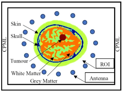
Figure 1. Configuration of the head model in 2D FDTD Scheme.
at timet=T. Figure 1 shows the numerical setup of an active microwave tomography. The FDTD cell size is given by Δx= 1 mm, Δy = 1 mm with a total cell size of 280×280 to complement the head phantom that consists of 16,413 points of reconstruction. This simulation space is bounded by 15 cells of Convolutional Perfectly Matched Layer (CPML) as absorbing boundary condition (ABC) has been used [24, 25]. 16 points of antenna are set up, elliptical in shape to minimize the gap variation between the head model and the antennas. The distance between the antennas and the head is varied from 20 mm to 28 mm. These variations are due to the irregular shape of the head model. These antennas are used as a transmitter sequentially while the other points act as receiving points for collecting data
˜
Vm(p;rn, t). Gaussian pulses with centre frequencies of 1 GHz and 2 GHz are utilized to illuminate the head phantom placed in a free space to ensure high penetration towards the head model.
The initial guess values are set at εr = 24.7 and σ = 0.19 denoted as the average of the total permittivity and conductivity value of the tissue types of the head model used. The simulations are carried out up to 100 iterations.
2.2. Focus Region with Image Segmentation
Segmentation is an important method that separates data into clusters. This method is used to classify various shapes of objects in an image. One of the segmentation methods, Otsu’s threshold segmentation method, is particularly a basic and powerful method to select and extract a region of interest (ROI) from the background (bi-level thresholding) on the basis of the distribution of grey levels in image [26–28]. This method will select the optimal threshold by maximizing between-class variance. Then, the result can be extended to output multilevel thresholding in order to increase the speed of computation [29]. In this work, the Otsu’s thresholding method is applied to process data of permittivity value of the head model instead of using standard image grey level range. The variance, σB2, is calculated by:
σ2B= d
k=1
ωk(μk−μT)2 (5)
wheredis the threshold value which is the maximum value of the brain image in terms of permittivity, ωk the cumulative probability of each data class,μk the mean for each class, andμT the mean weight of the data. The optimal threshold for different levels is chosen by:
t∗1, t∗2. . . , t∗d−1 = Arg MaxσB2 t1, t2, . . . , td−1
(6)
2.3. Head Model MRI 2D Derived Model
A homogeneous head model of an MRI simulated head data in 3D (.mnc format) is used with a size of 181×218×181 (in mm). The MRI data spatial resolutions are 1 mm3. A slice at z-axis 140 is chosen to get the 2D transverse plane view of the head model to test the FBTS technique. The data phantom contains 9 types of tissues which is later reduced to 4 significant tissues for the simulations, namely: skin, skull, WM and GM. The thicknesses of the skin, skull, WM and GM are in range of 9–12 mm, 5–12 mm, 3–24 mm and 3–13 mm, respectively. The fourth order Debye model parameters are as in Equation (7), mapped to each pixel of the 2D extracted MRI.
εr(ω) =ε∞+ 4
i=1
εSi−ε∞ 1+jωτi+
σs
jωε0 (7)
where, εr(ω) is the complex relative permittivity as a function of angular frequency, εSi the static permittivity at which the angular frequency, ω multiplies the relaxation time τi. ε0 denotes the permittivity of free space andε∞the permittivity at infinite frequency. The tumour location presented in this paper is fixed and embedded into the WM region as illustrated in Figure 2.
As mentioned in this paper, tumour size refers to the size of its diameter. Reconstruction of the brain image is based on the dielectric properties at 1 GHz and 2 GHz; therefore, the relative permittivity
Figure 2. Actual homogenous 2D head model with 5–15 mm tumour.
Table 1. Tissues permittivity and conductivity at 1.5 GHz.
Tissue εr (F/m) σ (S/m)
Skin 38.91 0.87
Skull 12.14 0.25
White Matter 36.90 0.95 Grey Matter 48.16 1.37
Tumour 59.90 1.65
Table 2. Tissues permittivity and conductivity at 1.5 GHz reduced by 30%.
Tissue εr (F/m) σ (S/m)
Skin 27.24 0.61
Skull 8.50 0.18
White Matter 25.83 0.67 Grey Matter 33.71 0.96
(c) (d)
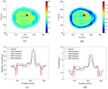
Figure 3. Reconstructed brain image with 15 mm tumour embedded at 1 GHz. (a) Reconstructed relative permittivity. (b) Reconstructed conductivity. (c) Cross-sectional view at y = 155 of reconstructed relative permittivity. (d) Cross-sectional view aty= 155 of reconstructed conductivity.
and conductivity for nominal Debye parameters evaluated at a frequency of 1.5 GHz are as in Table 1 [30– 32]. The permittivity and conductivity values are reduced by 30% of its originally obtained values from the Debye formula except for the tumour as described in Table 2. The reduction of the dielectric properties is due to the differences of water content in tissues, which correlates to age and can be roughly estimated up to 30% based on the data provided by Peyman [33, 34].
3. RESULTS AND DISCUSSION
(c)
(a) (b)
(d)
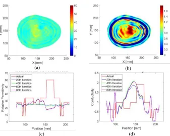
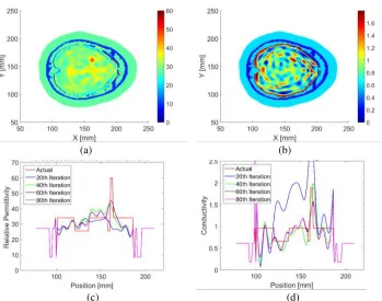
Figure 4. Reconstructed brain image with 15 mm tumour embedded at 2 GHz. (a) Reconstructed relative permittivity. (b) Reconstructed conductivity. (c) Cross-sectional view at y = 155 of reconstructed relative permittivity. (d) Cross-sectional view aty= 155 of reconstructed conductivity.
tumour.
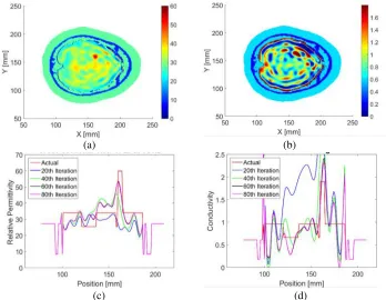
Figure 4 shows the results of illuminating the head model at 2 GHz. The reconstructions are poor compared to the results obtained at 1 GHz. The tumour is undetected due to a weak signal penetration. Also, the complexity of brain structure causes the estimation of 5 layers of tissues to become more difficult due to lack of information received at the receiver. Thus, it leads to an incorrect and inaccurate reconstruction which can be observed in Figures 4(c) and 4(d). The opposite results are obtained when the tumour sizes are reduced with less than 15 mm as shown in Figure 5 through Figure 7. The tumours embedded in the head model are detected by the algorithm for tumour sizes of 10 mm, 7 mm, and 5 mm; however, the detection becomes weaker as the tumour size is reduced to 5 mm. It is almost indistinct from the WM. These two cases prove that the weak signals penetration occurs at the tumour size greater than 15 mm due to the high relative permittivity of the tumour. It means that the signals penetration increases as the tumour size decreases.
(c) (d)
Figure 5. Reconstructed brain image with 10 mm tumour embedded at 2 GHz. (a) Reconstructed relative permittivity. (b) Reconstructed conductivity. (c) Cross-sectional view at y = 155 of reconstructed relative permittivity. (d) Cross-sectional view aty= 155 of reconstructed conductivity.
(c)
(a) (b)
(d)
(c)
(a) (b)
(d)
Figure 7. Reconstructed brain image with 5 mm tumour embedded at 2 GHz. (a) Reconstructed relative permittivity. (b) Reconstructed conductivity. (c) Cross-sectional view at y = 155 of reconstructed relative permittivity. (d) Cross-sectional view aty= 155 of reconstructed conductivity.
(c)
(a) (b)
(d)
(c) (d)
Figure 9. Reconstructed brain image with 10 mm tumour embedded at 2 GHz by integrating segmentation technique. (a) Reconstructed relative permittivity. (b) Reconstructed conductivity. (c) Cross-sectional view at y = 155 of reconstructed relative permittivity. (d) Cross-sectional view at y= 155 of reconstructed conductivity.
(c) (d)
(a) (b)
(c) (d)
(a) (b)
Figure 11. Reconstructed brain image with 5 mm tumour embedded at 2 GHz by integrating segmentation technique. (a) Reconstructed relative permittivity. (b) Reconstructed conductivity. (c) Cross-sectional view at y = 155 of reconstructed relative permittivity. (d) Cross-sectional view at y= 155 of reconstructed conductivity.
permittivity for the tumour are increased towards the actual values compared to the results obtained from the technique without focusing reconstruction region. In terms of location, size and shape, the estimation is accurate. The ability to detect the embedded tumour is degrading as the tumour getting smaller, but the results are better than the technique without image segmentation. From the results obtained through this research, a tumour size less than 5 mm diameter is merely undetectable, which is the reason that the results presented here are limited to 5 mm diameter. Detection of tumour according to the size depends on the frequency used as mentioned earlier. By increasing the frequency, it is able to detect a smaller tumour, but the tradeoff is weaker signal penetration. Throughout this research, the findings suggest that the optimum frequency for head imaging is at 2 GHz.
Both techniques used for the simulations, FBTS and FBTS integrated with image segmentation, are unable to reconstruct the GM and WM region at 2 GHz which requires an advanced technique to ensure better signals penetration to obtain sufficient information for reconstruction. Despite that, the primary objective is the ability to detect the embedded tumour at an early stage so that a further treatment can be done.
4. CONCLUSION
“The role of tumour size in the Radio Surgical management of Patients with ambiguous brain metastases,” Neurosurgery, Vol. 53, No. 2, 272–281, 2003.
4. Hossain, M. D., A. S. Mohan, and M. J. Abedin, “Beamspace time-reversal microwave imaging for breast cancer detection,” IEEE Antennas Wirel. Propag. Lett., Vol. 12, 241–244, 2013.
5. Mustafa, S., B. Mohammed, and A. Abbosh, “Novel preprocessing techniques for accurate microwave imaging of human brain,”IEEE Antennas Wirel. Propag. Lett., Vol. 12, 460–463, 2013. 6. Mobashsher, A. T., A. M. Abbosh, and Y. Wang, “Microwave system to detect traumatic brain injuries using compact unidirectional antenna and wideband transceiver with verification on realistic head phantom,”IEEE Trans. Microw. Theory Tech., Vol. 62, No. 9, 1826–1836, 2014.
7. Henriksson, T., N. Joachimowicz, C. Conessa, and J. Bolomey, “Quantitative microwave imaging for breast cancer detection using a planar 2.45 GHz system,”IEEE Trans. Instrum. Meas., Vol. 59, No. 10, 2691–2699, 2010.
8. Mohammed, B. J., A. M. Abbosh, S. Mustafa, and D. Ireland, “Microwave system for head imaging,”IEEE Trans. Instrum. Meas., Vol. 63, No. 1, 117–123, 2014.
9. Al Sharkawy, M., M. Sharkas, and D. Ragab, “Breast cancer detection using support vector machine technique applied on extracted electromagnetic waves,” Appl. Comput. Electromagn. Soc. J., Vol. 27, No. 4, 292–301, 2012.
10. Alqallaf, A. K., R. K. Dib, and S. F. Mahmoud, “Microwave imaging using synthetic radar scheme processing for the detection of breast tumours,”Appl. Comput. Electromagn. Soc. J., Vol. 31, No. 2, 98–105, 2016.
11. Bowman, T. C., A. M. Hassan, and M. El-shenawee, “Imaging 2D breast cancer tumour margin at terahertz frequency using numerical field data based on DDSCAT,” Appl. Comput. Electromagn. Soc. Journal, Vol. 28, No. 11, 1017–1024, 2013.
12. Takenaka, T., H. Jia, and T. Tanaka, “Microwave imaging of electrical property distributions by a forward-backward time-stepping method,” J. Electromagn. Waves Apllied, Vol. 14, No. 12, 1611–1628, 2000.
13. Takenaka, T., T. Moriyama, K. A. Hong Ping, and T. Yamasaki, “Microwave breast imaging by the filtered forward-backward time-stepping method,” 2010 URSI International Symposium on Electromagnetic Theory, 946–949, 2010.
14. Johnson, J. E., T. Takenaka, and T. Tanaka, “Two-dimensional time-domain inverse scattering for quantitative analysis of breast composition,”IEEE Trans. Biomed. Eng., Vol. 55, No. 8, 1941–1945, 2008.
15. Ping, K. A. H., T. Moriyama, T. Takenaka, and T. Tanaka, “Two-dimensional forward-backward time-stepping approach for tumor detection in dispersive breast tissues,”Mediterranean Microwave
Symposium, MMS 2009, 2009.
16. Cocosco, C. A., V. Kollokian, R. K. S., and A. C. Kwan, “BrainWe: online interface to a 3D MRI simulated brain database,” Neuro Image, Vol. 5, No. 4, 1997.
18. Canada, H., “Limits of human exposure to radio frequency electromagnetic energy in the frequency range from 3 kHz to 300 GHz,”Saf. Code, 2015.
19. Lin, J. C., “Safety standard for human exposure to radio frequency radiation and their biological rationale,” IEEE Microwave Magazine, Vol. 4, No. 4, 22–26, 2003.
20. Ping, K. A. H., T. Moriyama, T. Takenaka, and T. Tanaka, “Reconstruction of breast composition in a free space utilizing 2-D forward-backward time-stepping for breast cancer detection,” 4th IET International Conference on Advances in Medical, Signal and Information Processing (MEDSIP 2008), 313–313, 2008.
21. Yong, G., K. A. Hong Ping, A. Sia Chew Chie, S. W. Ng, and T. Masri, “Preliminary study of Forward-Backward Time-Stepping technique with edge-preserving regularization for object detection applications,” 2015 International Conference on BioSignal Analysis, Processing and Systems (ICBAPS), 77–81, 2015.
22. Ng, S. W., K. A. H. Ping, S. Sahrani, M. H. Marhaban, M. I. Saripan, T. Moriyama, and T. Takenaka, “Preliminary results on estimation of the dispersive dielectric properties of an object utilizing frequency-dependent forward-backward time-stepping technique,” Progress In Electromagnetics Research M, Vol. 49, 61–68, 2016.
23. Johnson, J. E., T. Takenaka, K. A. H. Ping, S. Honda, and T. Tanaka, “Advances in the 3-D forward-backward time-stepping (FBTS) inverse scattering technique for breast cancer detection,”
IEEE Trans. Biomed. Eng., Vol. 56, No. 9, 2232–2243, 2009.
24. Giannakis, I. and A. Giannopoulos, “Time synchronized convolutional perfectly matched layer for improved absorbing performance in FDTD,”IEEE Antennas Wirel. Propag. Lett., Vol. 14, 690–693, 2015.
25. Sullivan, D. M., Electromagnetic Simulations Using the FDTD Method, IEEE Press Marketing, New York, 2000.
26. Vala, H. J. and A. Baxi, “A review on Otsu image segmentation algorithm,” Int. J. Adv. Res. Comput. Eng. Technol., Vol. 1, No. 4, 387–389, 2013.
27. Otsu, N., “A threshold selection method from gray level histogram,” IEEE Trans. Syst. Man Cybern., Vol. 9, 62–66, 1979.
28. Khan, W., “Image segmentation techniques: A survey,” J. Image Graph., Vol. 2, No. 1, 6–9, 2013. 29. Liao, P. S., T. S. Chen, and P. C. Chung, “A fast algorithm for multilevel thresholding,” J. Inf.
Sci. Eng., Vol. 17, 713–727, 2001.
30. Mustafa, S., A. M. Abbosh, and P. T. Nguyen, “Modeling human head tissues using fourth-order Debye model in convolution-based three-dimensional finite-difference time-domain,” IEEE Trans. Antennas Propag., Vol. 62, No. 3, 1354–1361, 2014.
31. Yoo, D.-S., “The dielectric properties of cancerous tissues in a nude mouse xenograft model,”
Bioelectromagnetics, Vol. 25, No. 7, 492–497, Oct. 2004.
32. Thourn, K., T. Aoyagi, and J. Takada, “Numerical simulation of 2D scattering by a lossy dielectric cylinder using Debye modelling of absorbing material and pulse excitation source,”2015 7th Asia-Pacific Conference on Environmental Electromagnetics (CEEM), 165–168, 2015.
33. Peyman, A., S. J. Holden, S. Watts, R. Perrott, and C. Gabriel, “Dielectric properties of porcine cerebrospinal tissues at microwave frequencies: in vivo, in vitro and systematic variation with age,”
Phys. Med. Biol., Vol. 52, No. 8, 2229–2245, Apr. 2007.