BIROn - Birkbeck Institutional Research Online
Razgon, Igor (2016) On oblivious branching programs with bounded
repetition that cannot efficiently compute CNFs of bounded treewidth. Theory
of Computing Systems 61 , pp. 755-776. ISSN 1432-4350.
Downloaded from:
Usage Guidelines:
Please refer to usage guidelines at
or alternatively
On oblivious branching programs with bounded
repetition that cannot efficiently compute CNFs
of bounded treewidth
Igor Razgon
Department of Computer Science and Information Systems,
Birkbeck, University of London
[email protected]
Abstract
In this paper we study complexity of an extension of ordered binary decision diagrams (obdds) called c-obdds on cnfs of bounded (primal graph) treewidth. In particular, we show that for each k there is a class of cnfs of treewidth k ≥ 3 for which the equivalent c-obdds are of size Ω(nk/(8c−4)). Moreover, this lower bound holds if c
-obdd is
non-deterministic and semantic. Our second result uses the above lower bound to separate the above model from sentential decision diagrams (sdds). In order to obtain the lower bound, we use a structural graph parameter called matching width. Our third result shows that matching width and pathwidth are linearly related.
1
Introduction
Ordered Binary Decision Diagramsobdds is a famous representation of Boolean functions being actively investigated from both applied and theoretical perspec-tive. The theoretical research, among other things, has resulted in many upper and lower bounds ofobddsize realizing various classes of functions [14].
One such an upper bound, established in [7] states that a cnfof treewidth
k of its primal graph can be represented by an obddof size O(nk). In terms of parameterized complexity, this is anxp upper bound, that is the degree of the polynomial depends onk. A natural open question is whether this upper bound can be improved to anfptupper bound, i.e. one of the formf(k)∗nc, wherecis a universal constant.
This question is of a particular interest in the area of knowledge compilation because of the recent introduction of Sentential Decision Diagrams (sdds) [6] for which anfpt upper bounddoes hold. sdds share withobdds a number of nice properties and have a good potential to replaceobdds in applications. Yet
obdd-related machinery is much more developed (one reason for that is that obdds have been investigated for a much longer time) and hence it is interesting
to say if this gap between upper bounds can be significantly tightened by finding a better upper bound forobdds.
In [12], we answered this question negatively by demonstrating that for each
k ≥3 there is a class of cnfs of primal graph treewidth at mostk for which the size of equivalentobdds is Ω(nk/4). In this paper, which can be considered as a follow-up version of [12], our motivation is to see how far theobddcan be extended so that the above lower bound would hold for that extended model in a way that the lower bound in [12] would follow as a special case. As a result, we extend obdds as follows. First, for an arbitrary (but fixed) constant c we usec-obdds insteadobdd. That is, we allow each variable to occur at mostc
times along each computational path, however the occurrences are ordered asc
concatenated copies of the same fixed permutation (in this setting theobddis simply 1-obdd). Second, we allow the model to be non-deterministic. Roughly speaking, this means that instead of applying this restriction on a branching program, the restriction is applied on a switching and rectifier network. Third, we allow this restriction to besemantic, i.e to hold only forconsistentpaths that do not contain opposite occurrences of the same variables. The in-consistent paths are not constrained at all. We call the resulting model Nondeterministic Semanticc-obddand abbreviate itc-nsobdd. In particular, we show that for each fixedk≥3 there is a class ofcnfs (in fact, the same class as we used in [12]) for which the smallestc-nsobddis of size Ω(nk/(8c−4)). Clearly, the lower
bound forobdds follows if we substitutec= 1.
The above lower bound shows thatc-nsobdds are inherently different from
sddwith respect to representation ofcnfof bounded treewidth. Our second
re-sult shows that this difference can, in fact, be turned into a (non-parameterized) separation. In particular by, essentially, settingk to logn, we obtain a class of
cnfthat can be represented by polynomial sizesdds but require c-nsobddof
quasipolynomial size.
Our third result is related to the way the main lower bound is obtained. In particular, thecnfs we consider for the sake of obtaining lower bounds, corre-spond to undirected graphs. We introduce a graph parameter calledmatching width and show that the size of c-nsobddequivalent to the considered cnfis exponential in the matching width of the corresponding graph. Then we show that there are graphs for which the matching width is Ω(logn) times larger than their treewidth. The lower bound readily follows from the combination of these results. The relationship between matching width and treewidth suggests that the former issimilar to pathwdith. Our third result shows that this is indeed true, that is pathwidth and matching width are linearly related.
The last result might seem a little bit out of scope. The reason why we provide it in this paper is that matching width has already been used several time to obtain lower bounds [12, 11, 5]. So, it is interesting to see how it is connected to well known graph parameters. To the best of our knowledge [12] is the first paper where matching width for used for lower bounds, so a follow-up version of [12], seems the natural place for showing how matching width is connected to pathwidth.
with exponential lower bound provided for several functions. Thec-obddmodel is known to be more powerful than the ordinaryobdd. In particular, Theorem 7.2.2. of [14] provides a class of functions polynomial for 2-obddand exponential even for Free Binary Decision Diagrams (fbdd) (that is, read-once branching programs). Moreover, it is known that increse ofc adds computational power. In particular, it has been demonstrated in [3] that for each c ≥ 2 there is a class of functions computable by poly-size c-obdds and requiring exponential size c−1-obdds. Interesting refinements of this hierarchy involving width of branching programs have been proposed in [1, 9].
It is also known that non-determinism adds power to obdd. In particular, Theorem 10.2.3. of [14] demonstrates a class of functions that can be computed by poly-size non-deterministicobdds, yet require exponential size fbdds. We are not aware of the any existing researchspecifically on non-deterministic c
-obdds. They are obviously a special case of non-deterministic read k-times
branching programs and hence exponential lower bounds (e.g. [4]) apply to them. It is well known that semantic rather than syntactic restriction adds a lot of power if the obliviousness requirement is dropped. In particular, [8] demonstrates a class of functions that can be computed by poly-size semantic non-deterministic read-once branching programs but require exponential size if ‘semantic’ is replaced by ‘syntactic’. In fact, no super-polynomial lower bound is known for the former. We are not aware, however, if the semantic restriction adds any power to non-deterministicobdds. The lower bound of [12] has been generalized in [11] to a different direction than the one considered in this pa-per: namely the obliviousness was dropped. In particular, it has been shown that the non FPT lower bound holds for non-deterministic read-once branching programs.
Matching width can be seen as a special case of maximum matching width introduced in [13] when the underlying tree is a caterpillar. It has been shown in [13] that maximum matching width is linearly related to the treewidth. The linear relationship between matching width and pathwdith, established in this paper, looks natural in this context.
The rest of the paper is structured as follows. Section 2 introduces the necessary background. Section 3 states the lower bound on c-nsobdds along with the separation from sdd. The lower is proved in Section 4. The proof of linear relationship between matching width and pathwidth is provided in Section 5.
2
Preliminaries
where variables occurring positively inS (i.e. whose literals in S are positive) are assigned withtrueand the variables occurring negatively are assigned with
f alse.
A non-deterministic branching program Z is a directed acyclic graph dag
with one root rt and one leaf lf. Some of the edges of Z are labelled with literals of variables. A pathP of Z is consistent if it does not have two edges labelled with opposite occurrences of the same variable. This gives us possibility to defineA(P), the set of literals labelling the edges of a consistent pathP. A consistent root-leaf path ofZ is also called acomputational path. The function
Fcomputed byZis defined as follows. LetSbe an assignment to the variables of
Z. ThenSis a satisfying assignment ofF if and only if there is a computational pathP ofZ such that A(P)⊆S.
Special classes of non-deterministic branching programs can be defined by putting restrictions on properties of their root-leaf paths. A restriction is se-manticif it is applied tocomputational paths only andsyntacticif it is applied to all the root-leaf paths. In order to define the restriction we use in this paper, we need an additional notation.
Let SV be a permutation of variables and let S be a sequence of literals of (some) variables occurring in SV. We say that S is ordered according to
SV if for any two variables X and Y occurring in S, the occurrence of X is ordered before the occurrence ofY inS if and only ifS is ordered before Y in
V. For instance ifSV = (X2, X4, X5, X1, X3) then (¬X4, X5,¬X3) is ordered
according toSV.
Let P, P1, P2 be paths of a directed graph G. Then P = P1+P2 if P is
obtained by appendingP2to the end ofP1. For example, suppose that a path
is represented by a sequence of its vertices and letP = (v1, v2, v3, v4, v5). Then P= (v1, v2, v3) + (v3, v4, v5) and alsoP =P+ (v5) and alsoP= (v1) +P. This
definition is naturally extended to a a decomposition ofP =P1+. . . , Pk into an arbitrary number of paths.
We consider a class of non-deterministic branching programs Z for which there is a permutationSV of its variables and a constantcsuch that each com-putational (that is, the restriction is semantic) pathP ofZ can be represented asP =P1, . . . , Pc so that on eachPi each variable occurs at most once and the sequence of literals labelling the edges alongPi is ordered according toSV.
We call this class of branching programsNondeterministic Semanticc-obdd
and abbreviate itc-nsobdd. Notice that the ordering imposed on computational paths is more restrictive than the one imposed on read-c-times oblivious branch-ing programs. Indeed, in the latter case, variables can occur along a path in an arbitrary (though the same for all paths) order. In our case, however, the order of occurrences is determined by concatenation of c copies of the same
permutation of variables.
Given acnfF, itsprimal graph has the set of vertices corresponding to the variables ofF. Two vertices are adjacent if and only if there is a clause of F
where the corresponding variables both occur.
subset of V(G) and the bags obey the rules ofunion (that is, S
t∈V(T)B(t) =
V(G)),containment (that is, for each{u, v} ∈E(G) there ist∈V(t) such that
{u, v} ⊆B(t)), and connectedness (that is for each u∈V(G), the set of all t
such thatu∈B(t) induces a subtree ofT). The width of (T,B) is the size of the largest bag minus one. The treewidth of Gis the smallest width of a tree decomposition of G. If T is a path then (T,B) is a path decomposition The
pathwidth of a graph is the smallest width of its path decomposition.
V1
V1V2 V1V3
V1 V2 V3
V2 V3
V4 V5
V6 V7
V1
V4 V2
V1
V3 V5
[image:6.612.239.374.220.364.2]V7 V6
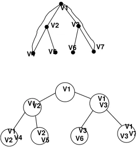
Figure 1: A graph and its tree decomposition
Figure 1 shows a graph and its tree decomposition. The width of this tree decomposition is 2 since the size of the largest bag is 3.
3
Lower bound parameterized by treewidth
In this section, given two integersr and k, we define a class of cnfs, roughly speaking, based on complete binary trees of height rwhere each node is asso-ciated with a clique of sizek. Then we prove that the treewidth of the primal graphs ofcnfs of this class is linearly bounded by k. Further on, we state the main technical theorem (proven in the next section) that claims that the small-est c-nsobddsize for cnfs of this class exponentially depends on rk. Finally, we re-interpret this lower bound in terms of the number of variables and the treewidth to get the lower bound announced in the Introduction.
Let G be a graph. A graph based cnf denoted by CN F(G) is defined as follows. The set of variables consists of variables Xu for each u∈ V(G) and variables Xu,v = Xv,u for each {u, v} ∈ E(G). The set of clauses consists of clausesCu,v=Cv,u= (Xu∨Xu,v∨Xv) for each{u, v} ∈E(G). In other words, the variables ofCN F(G) correspond to the vertices and edges ofG. The clauses correspond to the edges ofG.
mutually adjacent. DenoteCN F(CTr,k) byFr,k.
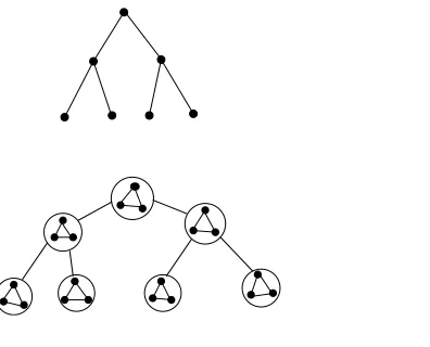
Figure 2: T2and CT2,3
Figure 2 shows T2 andCT2,3. To avoid shading the picture of CT2,3 with
many edges, the cliques corresponding to the vertices ofT2are marked by circles
and the bold edges between the circles mean that that there are edges between all pairs of vertices of the corresponding cliques.
Lemma 1 Letk≥2. Then the treewidth of the primal graph ofFr,k is at most 2k−1.
Proof. The primal graph of Fr,k can be obtained from CTr,k by adding one vertexve for each edgeeof CTr,k and making this vertex adjacent to the ends ofe. Let (T,B) be a tree decomposition of CTr,k of size at most 2k−1. For each vertexve, add a new vertex xto T adjacent to the vertex whose bag contains the ends of e. Associate with xa bag containing ve and the ends of
e. It is not hard to see that as a result we obtain a tree decomposition of the primal graph ofFr,k. Also, as the size of each new bag is 3 andk≥2, the width of the tree decomposition remains at most 2k−1. So, it remains to show that the treewidth ofCTr,k is at most 2k−1.
Consider the following tree decomposition (T,B) ofCTr,k. T is justTr. We look uponTr as a rooted tree, the centre ofTr being the root. The bag B(u) of each node u contains the clique of CTr,k corresponding to u. In addition, if u is not the root vertex then B(u) also contains the clique corresponding to the parent of u. Observe that (T,B) satisfies the connectivity property. Indeed, each vertex appears in the bag corresponding to its ‘own’ clique and the cliques of its children. Clearly, the set of nodes corresponding to the bags induce a connected subgraph. The rest of the tree decomposition properties can be verified straightforwardly. We conclude that (T,B) is indeed a tree decomposition of CTr,k. As the size of each bag is at most 2k, the width of (T,B) is at most 2k−1.
The following is the main technical result whose proof is given in the next section.
Theorem 1 The size ofobddcomputing Fr,k is at least2rk/(4c−2).
The following lemma reformulates the statement of Theorem 1 in terms of the number of variables ofFr,k andk.
Lemma 2 Letmbe the number of variables ofFr,k. Then the size ofc-nsobdd
computingFr,k is at least(6mk2)
k/(4c−2).
Proof. Recall that Tr has 2r+1−1 nodes. For each node a of Tr, Fr,k haskvariables corresponding to the vertices of the clique ofaplus k2
variables corresponding to the edges of this clique. In addition, ifais a non-root node then it is associated withk2variables connecting the clique ofawith the clique of its
parent. Thus each node ofTr is associated with at mostk+ k2+k2 variables and hence the total number of variablesm≤(2r+1−1)∗(k+ 2k+k2)≤2r∗6k2. Thus 2r≥ m
6k2.
It follows from Theorem 1 that the size of ac-nsobddcomputingFr,k is at least 2rk/(4c−2)= (2r)k/(4c−2)≥( m
6k2)
k/(4c−2)as required.
Two lower bound parameterized by the treewdith now easily follows.
Theorem 2 For eachp≥3there is an infinite sequence ofcnfs F1, F2. . . ,of
treewidth at most pof their primal graphs such that for each Fi the size ofc
-obddcomputing it is at least(3mp2)p/(8c−4), wherem is the number of variables
of Fi. In particular, for c = 1 and every fixed p, we get the earlier obtained
obddlower bound ofΩ(mp/4)as a special case.
Proof. For an odd p, consider the cnfsFr,(p+1)/2 for allr≥1 and for an
evenp, consider thecnfs Fr,p/2 for all r ≥1. By Lemma 1, the treewidth of
the primal graph ofFr,(p+1)/2 is at most pand of Fr,p/2 at mostp−1. Thus
the treewidth requirement is satisfied regarding these classes.
Taking into account Lemma 2 and performing simple algebraic calculation, we observe thec-nsobddsize is lower-bounded by (3mp2)p/(8c−4).
Theorem 1 also allows us to separate betweenc-nsobddand Sentential De-cision Diagramssdd[6] for every fixedc.
Theorem 3 There is an infinite family of functions that can be computed by SDDs of sizeO(n3)and for which the smallestc-NSOBDD are of size nΩ(logn)
(for each fixedc)
ProofConsider functions Fr,r. Let us compute the number n of variables ofFr,r. Following the calculation as in Lemma 2, we observe thatn= (2r+1− 1)∗(r∗(r2−1)+r) + (2r+1−2)∗r2= 2r(3r2+r)−5r2+r
2
Denote 3r2+rbyp
1 and 5r
2+r
2 byp2. Thenr= log
n+p2
p1 .
In particular, r ≥ logn−logp1 ≥ logn−r and hence r ≥ logn/2 for a
provided by Theorem 1 gives us lower bound 216log2c−n4 =n
log
16c−4 which is Ω(nlogn
for every fixedc.
On the other hand, for a sufficiently large n, r ≤log(n+p2)≤log(2n) =
logn+ 1. By Lemma 1, the treewidth of the primal graph of Fr,r is at most 2r−1 which is at most 2 logn+ 1 by the above upper bound. Thus, according to [6], the size ofsddfor Tr,r is bounded byO(22lognn) =O(n3), as required.
4
Lower bound parameterized by the matching
width
The central concept we use for the proof of Theorem 1 is that of matching width. A matchingM of a graph Gis a set of edges ofGsuch that no two edges are incident to the same vertex. LetSV be apermutation of the setV =V(G) of vertices of a graphG. LetS1 be aprefix ofSV (i.e. all vertices ofSV \S1are
ordered afterS1). Let us call thematching width ofS1, the size of the largest
matching consisting of the edges between S1 and V \S1 (we take the liberty
to use sequences as sets, the correct use will be always clear from the context). Further on, the matching width ofSV is the largest matching width of a prefix of SV. Finally the matching width of G, is the smallest matching width of a permutation ofV(G).
Example 1 Consider a path of10 verticesv1, . . . , v10 so that vi is adjacent to
vi+1 for1≤i <10. The matching width of permutation (v1, . . . , v10)is1 since
between any suffix and prefix there is only one edge. However, the matching width of the permutation(v1, v3, v5, v7, v9, v2, v4, v6, v8, v10)is5 as witnessed by
the partition{v1, v3, v5, v7, v9}and{v2, v4, v6, v8, v10}. Since the matching width
of a graph is determined by the permutation having the smallest matching width, and, since the graph has some edges, there cannot be a permutation of matching width0, we conclude that the matching width of this graph is 1.
The main ‘engine’ for establishing the lower bound for Theorem 1 is the following theorem, stating a lower bound on the size of ac-nsobdd.
Theorem 4 Let G be a graph of matching width at least t and let Z be a c
-nsobddcomputing CN F(G). Then|Z| ≥2t/2c−1.
Theorem 4 is proved in Section 4.1. In order use Theorem 4 for a proof of Theorem 1, we need an additional statement providing a lower bound on the matching width of graphsCTr,k (recallFr,k =CN F(CTr,k)).
Theorem 5 (Lemma 2 of [12]) For any r, the matching width of CTr,k is at
leastrk/2.
Proof of Theorem 1According to Theorem 4, the size ofZ implementing
Fr,k =CN F(CTr,k) is at least 2t/2c−1 where t is the matching width ofCTr,k
Replacetby the lower boundrk/2 on the matching width ofCTr,k provided by Theorem 5. The required lower bound 2rk/(4c−2)immediately follows.
4.1
Proof of Theorem 4
LetSV be a permutation of the vertices ofGwhereuprecedesv if and only if
XuprecedesXv in te underlying permutationSV∗ofZ. We refer toSV as the permutation ofV(G)correspondingtoZ. LetSV P be a prefix ofSV such that there is a matchingM ={{u1, v1}, . . . ,{ut, vt}}ofGsuch that all ofu1, . . . , ut belong toSV P and all ofv1, . . . vtdo not. Such a prefix exists by definition of matching width and our assumption that matching width ofGis at leastt.
LetSbe the set of all assignmentsSto the variables ofCN F(G) satisfying the following conditions.
• Each¬Xui,vi∈S for 1≤i≤t.
• For each 1≤i≤t, the occurrences of Xui andXvi have distinct signs (if
the former occurs positively the latter occurs negatively and if the former occurs negatively the latter occurs positively).
• All the variables besidesSt
i=1{Xui, Xui,vi, Xvi}are assigned positively.
Then the following statements are easy to observe.
Observation 1 1. Each S∈Sis a satisfying assignment ofS.
2. |S| ≥2t.
Proof. For the first statement, note that all the clauses (Xu∨Xu,v∨Xv) besides (Xui∨Xui,vi∨Xvi) are clearly satisfied byS because Xu,v is assigned
positively by construction. The clauses (Xui∨Xui,vi∨Xvi) are also satisfied by
Sbecause one ofXui,Xvi is assigned positively. This proves the first statement.
There are 2tways to assign variablesX
u1, . . . , Xut. By definition ofSeach
such assignment can be extended to an element of S and these elements are clearly all distinct. This proves the second statement.
In light of the first statement of Observation 1, for eachS∈Swe can identify a computational pathPS ofZ such thatA(PS)⊆S. For eachPS we are going to identify a sequence of its vertices of length at most 2c−1 and to show that for distinctS1, S2∈S, the sequences associated withPS1 and PS2 are distinct.
In light of the second statement of Observation 1, it will follow thatZ contains at least 2tsequences of nodes of length 2c−1. As the number of such sequences is at most|Z|2c−1, it will immediately follow that|Z| ≥2t/(2c−1).
In order to define a sequence of vertices associated with each PS, we need some preparation. Let P be an arbitrary computational path of Z and let
• Each variable occurs at most once as a label ofPi.
• The labels onPi are ordered according toSV∗.
Note that the requiredP1, . . . , Pcexists according to definition ofc-nsobdd. Further on, let P0
1, . . . , P20c be subpaths of P such that for each 1≤i ≤c, the following holds.
• Pi=P20i−1+P20i.
• For eachv∈SV P,Xv can occur only inP20i−1 (not inP20i).
• For eachv /∈SV P,Xv can occur only inP20i (not inP20i−1).
Note thatP10, . . . , P20c exists. Indeed, by definition ofSV P, all the variables
X1 = {Xv|v ∈ SV P} occur in SV∗ before all the variables X2 = {Xv|v /∈
SV P}. Therefore, if bothX1andX2occur onPi, we can identify the last edge eofPi labelled by a variable ofX1 and letP20i−1 to be the prefix ofPi ending at the head ofe. If only variables ofX1 occur on Pi then let P20i−1 =Pi and
P2i be the last vertex ofPi. If only variables ofX2 occur onPi then letP20i−1
be the first vertex ofPi and P20i =Pi. Finally, if no variables occur onPi, the partition can be arbitrary.
Letx1, . . . , x2c−1be the respective ends ofP10, . . . , P20c−1. We callx1, . . . , x2c−1
the separation vectorofPandP10, . . . , P2cthedecompositionofPw.r.t. x1, . . . , x2c−1.
Remark. Note that there may be more than one possibleP10, . . . , P20c sat-isfying the above conditions and hence P can have several separation vectors. We just pick an arbitrary one and call itthe separation vector.
The separation vectors of paths PS are these very sequences mentioned in the proof plan above. Now we are going to prove that distinct pathsPS have different separation vectors.
Lemma 3 LetS1, S2be two distinct elements ofS. ThenP =PS1andQ=PS2
have different separation vectors.
Proof. Assume thatPandQhave the same separation vector (x1, . . . , x2c−1).
Letui be a variable having opposite assignments inS1andS2. (Such a variable
necessarily exists because the assignments ofv1, . . . vtare determined by assign-ments of u1, . . . , ut. So, if the assignments if each ui has the same occurrence in bothS1 and S2, the same is true regarding each vi, and hence S1 = S2, a
contradiction). Assume w.l.o.g. thatui occurs negatively inS1 and positively
inS2.
LetP1, . . . , P2c andQ1, . . . , Q2c be the respective decompositions ofP and
Qw.r.t. tox1, . . . , x2c−1. LetP Qbe the path obtained fromP by replacement
of eachPj with evenj byQj.
Proof. We need only to verify that there is no variable occurring both positively and negatively onP Q. By definition ofS, each variableXu,vhas the same occurrence in bothS1andS2. AsA(P)⊆S1andA(Q)⊆S2,Xu,vcannot have distinct occurrences inA(P) andA(Q). By definition of the decomposition w.r.t. the separation vector, a variableXv with v ∈SV P cannot occur inQi with eveni. It follows that inP Q, Xv can only occur on P1∪. . . P2c−1 which
is a subgrpah ofP. AsP is a computational path, it does not contain opposite literals ofXv and hence neither does P1∪. . . P2c−1. Due to the same reason,
a variable Xv with v /∈SV P cannot occur on Pi with even i. It follows that in P Q Xv can only occur on Q2∪. . . Q2c which is a subgrpah of Q. As Q is a computational path, it does not contain opposite literals ofXv and hence neither doesQ2∪. . . Q2c.
Claim 2 A(P Q)is disjoint with{Xui, Xui,vi, Xvi}.
Proof. By definition of SXui,vi occurs negatively in bothS1 and S2 and
hence it cannot occur positively inA(P) nor inA(Q) and hence, in turn it cannot occur positively inA(P Q) composed of subpaths ofP andQ. Sinceui∈SV P, a literal ofXui cannot occur onQ2, . . . , Q2c(by definition of the decomposition
w.r.t. the separation vector). If a literal ofXui occurs on P1, . . . , P2c−1 then
it is an element ofS1and hence negative by assumption. Similarly, a literal of Xvi cannot occur onP1, . . . , P2c−1 (since vi ∈/ SV P). If a literal ofXvi occurs
onQ2, . . . , Q2c then it is an element ofS2 and hence negative (by assumption, Xui ∈S2 and hence¬Xvi∈S2 by definition ofS).
By Claim 1 and definition ofZ, an arbitrary extension ofA(P Q) is a satisfy-ing assignment ofCN F(G). By Claim 2, there is an extensionSofA(P Q) con-taining all of¬Xui,¬Xui,vi,¬Xvi. However,Sfalsifies clause (Xui∨Xui,vi∨Xvi)
existing since{ui, vi}is an edge ofG. This contradiction shows that our initial assumption thatPandQhave the same separation vector is incorrect and hence the lemma holds.
Proof of Theorem 4 It follows from Lemma 3 and the second statement of Observation 1 that there are at least 2t distinct separation vectors of com-putational paths of Z. Each separation vector is a sequence of nodes of Z. Clearly, there are at most Z2c−1 such sequences. That is 2t ≤Z2c−1. Hence Z≥2t/(2c−1), as required.
5
Matching width vs. pathwidth
In this section we will show that the matching width, mw(G), of a graph G
is linearly related to its pathwidth, pw(G). It particular, we will show that
pw(G)/2≤mw(G)≤pw(G) + 1.
Let us extend our notation. The maximum matching size of a graph Gis denoted by ν(G). Let SV = (v1, . . . vn) be an ordering of vertices of G. For
of verticesV(G) and the set of edges{{u, v}|{u, v} ∈E(G), u∈Vi, v∈ ¬Vi}. In other words the edges ofGiare exactly those edges ofGthat have one end inVi and one end in¬Vi. With this notation in mind, the matching widthmwSV(G) ofSV can be stated as follows.
mwSV(G) =maxni=1ν(Gi) (1) If we denote bySVthe set of all permutations of vertices ofGthen
mw(G) =minSV∈SVmwSV(G) (2) Recall that a vertex cover (VC) of graphGis a set of vertices incident to all of its edges. The smallest size of vertex cover ofGis denoted by τ(G).
Observe that eachGi is a bipartite graph becauseVi and ¬Vi, partitioning its set of vertices are indepdent sets ofGi. It is well known that for a bipartite graph the size of the smallest vertex cover equals the size of maximum matching, that isν(Gi) =τ(Gi). HencemwSV(G) can be restated as follows
mwSV(G) =maxni=1τ(Gi) (3)
Now we are bready to prove an upper bound onmw(G).
Theorem 6 For any graphG,mw(G)≤pw(G) + 1.
Proof. Let (P,B) be a path decomposition of G of width pw(G). Let
x1, . . . , xm be the vertices of P chronologically listed as they occur along P. Recall thatB={B(x1), . . . , B(xm)}are the bags of the decomposition and the size of each bag is at mostpw(G) + 1.
Now we are going to define a permutation SV of V(G) for which we will show that mwSV(G) ≤pw(G) + 1, which will imply the theorem because, by definitionmw(G)≤mwSV(G).
Foru∈V(G), letf(u) be the smallest numberisuch thatu∈Bxi. LetSV
is an arbitrary permutation ofV(G) such thatu <SV v wheneverf(u)< f(v). It is not hard to see that such an order indeed exists. For instance, SV can be created as follows. Arbitrary order the vertices ofB(x1). For each 1< i≤ n, suppose that the vertices B(x1)∪ · · · ∪B(xi−1) have been already ordered
and letSV0 be the corresponding permutation. Then create a permuation of
B(x1)∪· · ·∪B(xi) by arbitrary ordering the vertices ofBxi\SV
0 and appending
them to the end ofSV0.
We are going to show that for each 1≤i < n,B(xf(vi)) is a vertex cover of
Githat is for each{u, v} ∈E(Gi) eitheru∈B(xf(vi)) oru∈B(xf(vi)). Observe
that this will imply the desired statement thatmwSV(G)≤pw(G) + 1. Indeed, by definition, there is 1≤i < nsuch thatmwSV(G) =τ(Gi). Combining with the claim we are going to prove, we will have
mwSV(G) =τ(Gi)≤B(xf(vi))≤pw(G) + 1 (4)
Pick 1 ≤i < n and let {u, v} ∈ E(Gi). Assume w.l.o.g. that u∈ Vi and
v ∈ ¬Vi. Then, by definition of SV, f(u) ≤ f(vi) and f(v) ≥ f(vi). If the
equality occurs regarding any of them, sayf(u) =f(vi) then, by definition of function f, u ∈ B(xf(u)) = B(xf(vi)). Thus it remains to consider the case
wheref(u)< f(vi) andf(v)> f(vi).
By the containment property of the path decomposition, there isjsuch that
{u, v} ⊆B(xj). By definition off(v),f(v)≤jand hencef(vi)< j. To preserve the connectedness property,umust occur in all bags B(xr) for f(u)≤r≤j. In particular, sincef(u)< f(vi) andf(vi)< j,u∈B(xf(vi)), as required.
Next we are going to show that pw(G)≤2∗mw(G). For this we need the following definition.
Definition 1 Let SV be a permutation of V(G). For eachGi, 1≤i < n, let
V Ci be a smallest VC of Gi. The setsV C1, . . . , V Cn−1 are called settledw.r.t. SV if for each1≤i < n−1,V Ci∩ ¬Vi⊆V Ci+1
The following lemma is proved in Section 5.1.
Lemma 4 For each permutation SV of V(G)there are V C1, . . . , V Cn−1 that
are settled w.r.t. SV.
Now we are ready for the theorem.
Theorem 7 For any graphG,pw(G)≤2mw(G).
Proof. LetSV = (v1, . . . , vn) be a permutation ofV(G) such thatmwSV(G) =
mw(G). LetV C1, . . . , V Cn−1be the smallest VCs ofG1, . . . , Gn−1, respectively,
that are settled w.r.t. SV.
Our candidate for path decomposition of width 2mw(G) is a pair (P,B) whereP is a pathx1, . . . , xn andBis a set of bagsB(x1), . . . , B(xn) defined as follows.
• B(x1) =V C1∪ {v1}.
• For 1< i < n,B(xi) =V Ci−1∪V Ci∪ {vi}.
• B(xn) =V Cn−1∪ {vn}.
In the rest of the proof we demonstrate that (P,B) is indeed a path de-composition ofGhaving width at most 2mw(G). This amounts to proving the following statements.
• (P,B) satisfies the union property. Indeed, by construction, for 1≤i≤n,
vi∈B(xi).
• (P,B) satisfies the containment property. Indeed, let {vi, vj} ∈ E(G) and assume w.l.o.g. that i < j. This means that {vi, vj} is an edge of each ofGi, . . . , Gj−1 and hence each ofV Ci, . . . , V Cj−1 has a non-empty
Assume thatvj∈V Ci. Then, by construction,{vi, vj} ∈B(xi), satisfying the containment property. Assume next that vi ∈ V Cj−1. Then, by
construction, {vi, vj} ∈ B(xj), satisfying the containment property. If none of the above assumptions hold then vi ∈ V Ci and vj ∈ V Cj−1. It
follows that there isi≤j0 < j−1 such thatvi∈V Cj0 andvj ∈V Cj0+1.
Then by construction, {vi, vj} ∈ B(xj0+1), satisfying the containment
property.
• (P,B) satisfies the connectedness property. Assume by contradiction that the connectedness property is violated. That is, there is a vertex uand
i, j > i+ 1 such thatu∈B(xi),u /∈B(xi+1), andu∈B(Xj). We assume
thatj is smallest possible subject to this property, that is,u /∈B(xj−1).
Sinceu /∈B(xi+1),u /∈V Ci. That isu∈B(Xi)\V Ci⊆V Ci−1∪ {vi}. It follows thatu∈Vi. Indeed, ifu=vi, this follows by definition ofVi. Otherwise, notice that since V C1, . . . , V Cn are settled, V Ci−1∩ ¬Vi ⊆
V Ci. As we know that u /∈V Ci, we conclude that u ∈ V Ci−1\ ¬Vi =
V Ci−1∩Vi
As u /∈V Cj−1, NGj−1(u)⊆V Cj−1. By Definition 1, NGj−1(u)∩ ¬Vj ⊆
V Cj. We claim that NGj(u) ⊆ NGj−1(u)∩ ¬Vj. This claim will imply
that NGj(u) ⊆V Cj and hence u /∈ V Cj by the minimality of V Cj (as
all the neighbours of uare already there). This is a contradiction to our assumption, confirming correctness of the connectedness property. It thus remains to prove the claim.
Let v ∈ NGj(u). As i < j and u ∈ Vi, u ∈ Vj and hence v ∈ ¬Vj.
Consequently,v∈ ¬Vj−1. As i < j−1,u∈Vj−1. Thus{u, v}is an edge
ofGwith one end inVj−1, the other in¬Vj−1. Hence{u, v}is an edge of Gj−1, that is v ∈NGj−1(u) confirming the claim and the connectedness
property as specified in the previous paragraph.
• The width of (P,B) is at most 2mw(G). That is, we have to show that for each 1≤i≤n,|B(xi)| ≤2mw(G) + 1. By definition, |V Ci|=τ(Gi) for 1 ≤ i < n. According to ((3)) τ(Gi) ≤ mwSV(G). Thus, in our case, |V Ci|=τ(Gi)≤mw(G). It follows that for 1 < i < n, |B(xi)| ≤
|V Ci−1|+|V Ci|+ 1≤2mw(G) + 1. Clearly, the same upper bound applies toB(x1) andB(xn).
5.1
Proof of Lemma 4
LetG= (U, V, E) be a bipartite graph with set of verticesU∪V and the set of edgesE, all having one end in U the other end inV. In order to prove Lemma 4, we need the following three auxiliary statements.
Proof. V C0\X is a VC of G\X. Indeed, none of the edges coveredG\X
are covered byX and hence they are covered byV C0\X.
If we assume thatV C00∪X is not a smallest VC ofGthen|V C0|<|V C00∪X|. That is,|V C0\X|+|X|=|V C0|<|V C00∪X|=|V C00|+|X|, from where we conclude that|V C0\X|<|V C00|. That is,V C0\X is a VC ofG\X smaller thanV C00 in contradiction to the definition ofV C00.
Lemma 5 Let G= (U, V, E) be a bipartite graph and let X ⊆V be such that there isV C1, a smallest VC ofG, such thatX ⊆V C1. LetY ⊆V. ThenG\Y
has a smallest VC being a superset ofX\Y.
Proof. Assume that the lemma is not true. Further on, assume thatY is a largest possible subset ofV for which the lemma does not hold.
Let us represent V C1 as V C10 ∪V C100 where V C10 consists of all vertices of V C1 incident to the edges ofG\Y andV C100 consists of all vertices incident to
edges ofG[U ∪Y]. Denote V C10 ∩V C100 by P R. Observe that both V C10 and
V C100 are VCs ofG\Y and G[U ∪Y], respectively. Indeed, each edgeeof, say
G\Y is covered byV C but it can be covered only by a vertex ofV C incident to it and this vertex belongs to V C10 by definition. Note also that P R ⊆ U.
Indeed, an edge ofG\Y and and edge ofG[U∪Y] cannot have a joint end that belongs toV.
LetV C1∗ be a smallest VC ofG\Y. Observe that P R\V C1∗6=∅. Indeed, assume the opposite, that is we assume thatP R⊆V C1∗. Note thatV C1∗∪V C100
is a VC of G as each edge of G is an edge of either G\Y or of G[U ∪Y]. Note further that sinceP R⊆V C1∗,V C1∗∪V C100=V C1∗∪(V C100\P R). Now, as V C1 is a smallest VC of G by definition, |V C10|+|V C100\P R| = |V C1| ≤
|V C1∗∪(V C100\ P R)| ≤ |V C1∗|+|V C100 \P R| from where we conclude that
|V C10| ≤ |V C1∗| and hence V C10 is also a smallest VC of G\ Y. However, this is a contradiction because X \Y ⊆ V C10. Thus we have confirmed that
P R\V C1∗6=∅.
LetY0 =NG\Y(P R\V C1∗). Note thatY0 is not empty as by definition of P Ris element of it is incident to an edge ofG\Y. Furthermore, asP R⊆U,
Y0⊆V and disjoint withY by definition. That is|Y∪Y0|>|Y|. By maximality ofY, there is a smallest VCV C2ofG\(Y ∪Y0) that includesX\(Y ∪Y0) as
a subset. As elements ofY0 incident to edges ofG\Y whose other ends are not contained inV C∗
1,Y0 ⊆V C1∗. Thus by Proposition 1, V C2∪Y0 is a smallest
VC ofG\Y. However, (X\Y) = ((X\Y)\Y0)∪((X\Y)∩Y0)⊆V C2∪Y0 .
providing contradiction to our initial assumption and completing the proof.
Lemma 6 Let G= (U, V, E) be a bipartite graph. LetY ⊆V and let X ⊆U
be such thatX is a subset of a smallest VC ofG\Y. Then X is a subset of a smallest VC ofG.
Proof. Let V C1 be a smallest VC ofG. IfX ⊆V C1, we are done.
Oth-erwise, we will show that there is another smallest VC ofG includingX as a subset.
Observe thatE(G\V C100) =E((G\Y)\P R). Indeed, ife∈E(G\V C100) then
e∈E(G\Y) (recall from the proof of Lemma 5 thatV C100 covers all the edges ofG[U ∪Y]. Moreover, since P R⊆V C100, e∈ E((G\Y)\P R). Conversely,
suppose that e ∈ E((G\Y)\P R). Then e is not covered by any vertex of
V C100 (as all the vertices ofV C100covering edges ofG\Y belong toP R). Hence e∈G\V C00
1.
Recall thatP R⊆U. SinceG\Y has a smallest VC includingX, it follows from Lemma 5 (applied toG\Y with playing the role ofGandY playing the role ofU for the substitution into the statement of Lemma 5) that (G\Y)\P R
has a smallest VCV C2includingX\P R. Employing the previous paragraph we
observe thatV C2is also a smallest VC ofG\V C100. By Proposition 1,V C2∪V C100
is a smallest VC ofGincludingX becauseX = (X\P R)∪P R⊆V C2∪V C100
as required.
Proof of Lemma 4. Let V C1 be an arbitrary smallest VC of G1. For
1≤i < n, having constructedV Ci, we constructV Ci+1
First we observe that Gi\vi+1 = Gi+1\vi+1. By Theorem 5, Gi\vi+1
has a smallest VC including (V Ci∩ ¬Vi)\ {vi+1} = V Ci ∩ ¬Vi+1. Next, by
Theorem 6, Gi+1 has a smallest VC including V Ci∩ ¬Vi+1. Set V Ci+1 to be
such a smallest VC. This construction guarantees the required property for all
i.
References
[1] Fardid M. Ablayev and Kamil R. Khadiev. Extension of the hierarchy for k-obdds of small width. Russian Mathematics, 57(3):46–50, 2013.
[2] Hans L. Bodlaender and Rolf H. M¨ohring. The pathwidth and treewidth of cographs. SIAM J. Discrete Math., 6(2):181–188, 1993.
[3] Beate Bollig, Martin Sauerhoff, Detlef Sieling, and Ingo Wegener. Hierarchy theorems for kobdds and kibdds. Theor. Comput. Sci., 205(1-2):45–60, 1998.
[4] Allan Borodin, Alexander A. Razborov, and Roman Smolensky. On lower bounds for read-k-times branching programs. Computational Complexity, 3:1–18, 1993.
[5] Simone Bova, Florent Capelli, Stefan Mengel, and Friedrich Slivovsky. Ex-pander cnfs have exponential DNNF size. CoRR, abs/1411.1995, 2014. [6] Adnan Darwiche. SDD: A new canonical representation of propositional
knowledge bases. InIJCAI, pages 819–826, 2011.
[7] Andrea Ferrara, Guoqiang Pan, and Moshe Y. Vardi. Treewidth in verifi-cation: Local vs. global. InLPAR, pages 489–503, 2005.
[9] Kamil Khadiev. Width hierarchy for $k$-obdd of small width. Electronic Colloquium on Computational Complexity (ECCC), 22:48, 2015.
[10] Matthias Krause. Lower bounds for depth-restricted branching programs.
Inf. Comput., 91(1):1–14, 1991.
[11] Igor Razgon. No small nondeterministic read-once branching programs for cnfs of bounded treewidth. In IPEC, pages 319–331, 2014.
[12] Igor Razgon. On OBDDs for CNFs of bounded treewidth. InPrinciples of Knowledge Representation and Reasoning(KR), 2014.
[13] Martin Vatshelle.New width parameters of graphs. PhD thesis, Department of Informatics, University of Bergen, 2012.