Some Global Algorithms of Random Search. Examples of Solving Problems

(1)

International Journal of Emerging Technology and Advanced Engineering

Website: www.ijetae.com (ISSN 2250-2459, ISO 9001:2008 Certified Journal, Volume 6, Issue 12, December 2016)

79 Some Global Algorithms of Random Search. Examples of

Solving Problems

George Filatov

Professor, Doctor of Techn. Sciences, Ukrainian State University of Chemical Technology, Ukraine

Abstract - This article in some degree is a review. In it is represented some global random search algorithms designed to solve complex problems of nonlinear programming. Is considered the setting of algorithms, testing on examples of solving specific problems for which the solution is known. Are adduced the independent and stepper algorithms of random search with different distribution of random trials, gullied algorithms and algorithm with the return after a failed step. Is considered the algorithm, that implements the synthesis of random search and dynamic programming at the optimization of multivariable systems.

Keywords — Nonlinear Programming, Random Search, Global Algorithms.

I. THE ALGORITHM WITH THE RELEASE OF

"SUSPICIOUS"SUB-AREA ON THE PRESENCE OF

GLOBAL EXTREMUM

The algorithm that is outlined below, allows reduction of number of trials on search using the preliminarily "reconnaissance" about the location of the global extremum. For a broad class of complex objects for optimization can build a distribution law of quality

function

F

 

X

in the assumption that the states

X

are selected in accordance with a uniform law of distribution across the search area. Thus, if the quality function can be provided in the form of:

 

_

 



m

i i

f

F

1

X

, (1)

Where the functions

f

_i

 

X

are loosely coupled, then at large number of variables in accordance with the limit theorem of probability theory, the value of

F

is distributed on a normal law [1].

One way or another, but it is assumed that the

distribution law

p



F

/

A



is known to an accuracy of a number of parameters

A





a

₁

,

a

₂

,....,

a

_k



of this

distribution (e.g., for normal distribution, two parameters is necessary to know: the mathematical expectation and variance). This makes it possible to build such a global search procedure [2].

We divide the entire search area on sub-areas, and we find out in which of them is most advantageous to place a specified number of tests to determine the state in which the quality function has the smallest value. As the selection criterion sub-area naturally take the mathematical expectation of lower sample value corresponding to a given number of tests in this sub-area.

The estimation of unknown value

M

for each sub-area is required a certain number

L

of test trials are needed to assess the distribution of parameters



s



i

1 

1 ,

2 ,...,

A

in each sub-area. With this evaluation, it is possible to determine the mathematical

expectation

M

_i of the smallest value of

F

at the distribution in each area of a specified number of tests

N

. Is required, at the minimum number of trials

L

find the sub-area which would meet with the probability of not less than a predetermined, lowest value

M

. The selected thus sub-area taken as the initial, etc.

The search process thus reduces to determining of the most promising sub-area that subsequently is divided on the following sub-areas or in it are accommodated all of the remaining trials. As you can see, the optimum search needs in an optimal dividing of the entire stock of trials on the "reconnaissance" that allows you to determine the most advantageous sub-area. Part of the remaining trials is evenly distributed in the selected sub-area.

II. THE ALGORITHM OF SLIDE ELLIPSE (ASE) This algorithm has been suggested by the authors of article [3].

The algorithm is described of recurrent expression:



_



_

 

_{ }

















  

i i

i

i i

f

X

1 1 1

at

,

at

,

(2)

 

X

f

 the penalty function in the form

(2)

International Journal of Emerging Technology and Advanced Engineering

80 F

 

X

 quality function;

 

_

_



I

i

g

_i

X

0 ,

 restrictions. Functions

 

X

F

and

g

_i

 

X

assumed to be continuous in hyper-parallelepiped:





_

X

, (4)





i1

,



i2

,...,



in





Ξ

 random vector whose

components are not correlated, and are determined by the relation  







 





n k y k k i jk

ij

a

e

1

1 Z

R



, (5)



z

1

,

z

2

,....,

z

n





Z

the vector uniformly

distributed on the unit n-dimens



R

₁

,

R

₂

,....,

R

_n





R

 vector lengths of the semiaxes of the ellipsoid given a priori;

A

 i



 

a

 _jki  transition matrix from the basis of the ellipsoid to the main basis of the space.

It is envisaged that the center of the ellipsoid to the i-th step is located at the point

X

_i, and the orientation of the axes depends on the results of previous steps. The value

y

is normally distributed with zero mean and variance

i



:

 

_

















2 2

2 exp

2

1

i i

y

f





. (6)

The lengths of the semiaxes of the ellipsoid are selected as comparable to the size of the field (4), and the dispersion varies according to the recurrence relation [2]:























 i i i

v

d

i 1 2 1 1

exp

1





, (7)

Where: 2 1 1 2 , 1



































  n j j j i ij i

R

x



,

v

_ij 

absolute value of the central point

y

for



_i:











2

2 exp

2

0 2 2 1 i i i i

dx

x

v

_





















_

.

In equation (7) the parameters

d

₁ and

d

₂ 

of forgetting and learning



0 

d

₁



1 ;

d

₂



0 

. In the transition to the new center of search

X

_i_₁



X

_i the first axis of ellipsoid is rotated in the direction:

i i i i i i

i

d

X







   1 1 4 3 1

_



, (8)

where



_i  the former direction of the axis

R

₁. Use of (7) involves stretching along the axis of an ellipsoid

1

R

. To build a complete orthonormal basis may be used the reception of orthogonalization [5] of the system of

linearly independent vectors, since



_i_₁.

In case of violation of constraints (4), we obtain:

     





















_j i ij j ij j ij i ij j ij

x

if

,

if

,

;

if

,

. (9)

The algorithm (2)-(9) is an algorithm of the slide ellipse (ASE). If the sizes of the ellipsoid are such that he completely covers the region (4), in view of that the

function

f

 

X

is continious then all the conditions of the theorem on convergence are performed [6] and the algorithm ASE at

i





with probability unit finds the



 neighborhood







0 

of the global minimum of the function

f

 

X

. The algorithm has the smoothing properties in comprehension of [7] and it is therefore is quite universal, is needed only the continuity of function

 

X

f

. At the same time, as already noted, ASE allows to find a global extremum.

Consider the application of the algorithm of the sliding of the ellipse to the solution of the general problem of mathematical programming. Following [8], we can write the general problem of mathematical programming:



X



min



F

(10)

 

_

_i

_

_I



g

_i

X

0 ,

(11)

 

n

i

I

E

(3)

International Journal of Emerging Technology and Advanced Engineering

81

where

g

_i

 

X

 a continuous function satisfying the Lipschitz condition with constant L:

 

X

1



g

 

X

2



L

X

1



X

2

g

_i _i , and

F

 

X



unimodal function in space. To solve this problem is proposed in [15] apply the random search algorithm using ASE under the scheme:

1. The starting point

X

₀, which is the permissible solution of the problem, is selected. Let us call

n

E



X

the solution



permissible for selected

0 



_, if

 

0

,

;

,

i

I

g

i

I

g

_i

X







 _i

X







.











L









X

_k

,



0

we find such

m



permissible solutions of problem

     

,

,...,

,

2

1 m

k k

k

X

such that





0

1









m

j

k j k

j

X



. (13)

The resulting system of linearly independent vectors is complemented by random vectors. This system of vectors with probability one is linearly independent. After the ortho-normalizing, we obtain a basis of space with the center in point. This basis we'll call temporary.

4. In the temporary basis we organize the search using ASE with the length of axis

n m

m

R

₁



₂



₃



....



_₁



....

Where

L

R

_n





. As the initial position of ellipsoid's

basis is taken the point

X

_k. In the process of the work of ASE his first axes remain in the subspace formed by the vectors (10). At this the penalty function is transformed to the form

 



 



p i

g

F

f

X



X



max

X

/



2 (14)

p

a natural number.

−4, is repeated. As a stopping criterion of the algorithm we can use the criterion proposed in [9].

Therefore, the introduct



permissible solutions can be applied to the problem (10)-(12) the random search method, stipulating the less stringent

conditions for the functions

F

and

g

_i (the differentiation of

F

,

g

_i and the continuity of

f

are not needed). Therefore, this algorithm is applicable to a wider class of problems than algorithms proposed in [8,10].



permissible solutions also allows to apply the theorem on convergence [6], and, as a consequence, with probability unit to find the solution of the problem (10)–( 12).

Described algorithm is illustrated by the example of weight optimization of the rod system of frame type (including buckling of compressed rods). The task was formulated in this way in [11]: minimize:

 

,

8

1



_



n

x

F

n

j j

X

. (15)

At the performance of restrictions:

 

0

33 32 31

23 22 21

13 12 11



r

D

X

. (16)

(4)

International Journal of Emerging Technology and Advanced Engineering

82

Таble 1

The results of the weight optimization of rod system of frame-type

The optimum values of

variables Random search

The method of gradient projection

1

x

0,05 0,18731

2

x

0,05 0,18684

3

x

0,13637 0,218590

4

x

0,05 0,18865

5

x

0,05 0,21311

6

x

0,0593 0,20662

7

x

0,3049 0,39264

8

x

0,24056 0,19728

 

X

F

0,94115 1,79111

The problem was solved with a computer at such

search parameters

;

6 ,

0 ;

2 ,

0 ...

;

1

₂ ₇ ₁ ₂

1



R



R



d



d



R

005 ,

0 ;

1

4

3



d







d

; the initial value of the dispersion of search was taken 0.5; the starting point of

search

x

_i



0 .

25 ,

1 ,

2 ,....,

8

. On variables were imposed the restrictions

0 .

05 

x

_i



1

0,. The decision, which was obtained through 31 iterations, is provided in Table 1. For comparison shows the data out of work [11], which were obtained by Rosen's gradient projection method.

As can be seen from Table 1, the criterion of quality

function

F

 

X

, that has been determined by random search method, is much of less than criterion of quality, that has been obtained by the method of gradient projection. The effectiveness of random search method is equal 47.5%.

III. THE ALGORITHM WITH ANON-UNIFORM STRAIN OF

DENSITY OF DISTRIBUTION OF SAMPLING POINTS

The analysis of ASE work [2] allowed to establish one of the feature associated with the method of determining

the function

p

_N

 

Ξ

. As already noted, for the interior points of the ellipsoid, the center of which is located at the point, corresponding to the last best sample, the

function

p

_N

 

Ξ



0

. The dimensions of ellipsoid, commensurability the length of its axes with dimensions of search area is a measure of inertia and globality of algorithm.

With a relatively small size of the ellipsoid the search stops in a local minimum. If the axis sizes are much larger than dimensions of the area of search, then there is a high probability of the appearing of sampling points behind the borders of region and in the presence of the type of restrictions

0 

x

_j



1 ,

j



1 ,

2 ,...,

n

, exists a high probability of selecting a limit point.

Based on these arguments, we construct an algorithm independent random search with a function

p

_N

 

Ξ



0

for internal points of the unit hypercube

x

_j



 

0 ,

1

, and

 

Ξ



0

N

p

for all the other points that do not satisfy

the condition

x

_j





_j



 

0 ,

1

. The density

p

_N

 

Ξ

is formed by of coordinatewise reflection the multidimensional normal law with zero mathematical

expectation and identical variance



_N in all axes. At this is displayed only a part of the initial of the normal law, that is enclosed in the cube with a side of [−1,1]. The boundary of this hypercube is displayed on the border with the side of [0,1], and the center of initial

N

X

, is received resulting from previous research stages.

Let

Ξ

_N







_N_,₁

,



_N_,₂

,....,



_N_,_n



, the coordinates



N N Nn



N



r

,1

,

r

,2

,....,

r

,

r

of a normal distribution

with parameters



0 ,



_N



and coordinates of the point N

(5)

International Journal of Emerging Technology and Advanced Engineering

83 























1

0 if

1

0

1 if

,

, ,

,

, ,

j N j

N j N

j N j

N j N j N

r

x

r

x



(17)

The function

p

_N

 

Ξ

, obtained at this, has the property that all direction coming out of the point

X

_N, identical on probability, however, the probability density in any direction decreases depending on the distance to the boundary of the unit hypercube with sides [0,1].

At each



_N



0

for all points of this hypercube

 

Ξ

N

p

is different from zero. In the process of search the dispersion is proposed to change by the rule:

0 ,

1

0 ,

₁

1 1

1













 N N N q

N

d



d

X

d



. (18)

Since the initial normal law defined on the whole space, and displays only a part without "tails", let us limit from above

the change



_N





so that:

1

0 ,

2

2 exp

2

3 3

1

2 2

























 









dr

r

x

N

. (19)

At the practical implementation of the algorithm can be accepted





0 ,

3

(from the condition



3 



1 

.

If



_N





 



₁ it is easy to make sure in the validity of the assertion that a sequence

 

X

_N satisfies (1.42).

IV. THE GULLIED ALGORITHM OF INDEPENDENT

GLOBAL SEARCH

The proposed global search algorithm with controlled density of distribution within allowable area as well as the algorithm of the sliding ellipse is the algorithm of independent search which is able to find a global extremum. However, unlike the ASE this algorithm allows to find extremum on the bottom of ravines arbitrary shape. For this purpose is introduced the basis, which is rotated, and allows to orient the axis along the bottom of curved ravine at each step. The difference between the considered algorithm of ASE is also in the selection of the distribution of test density. For ASE the

distribution density



 

Ξ

takes positive values at interior points of the ellipsoid with a center in the last better point of search. The measure of inertia and necessary condition of globality at the using of ASE are the dimensions of ellipsoid - the commensurateness the length of its axes with the dimensions of the search area. If the axis sizes are much larger than the area D (the area of the existence of the objective function), there is a high probability of appearance the trials overseas area, and at the presence of constraints such as:

x

_j



x

_j



x

_j

,

j



1 ,

2 ,...,

n

, (20)

a high probability of selecting a limit point of type 

j

x

.

In view of these considerations was created the algorithm, which uses



_N

 

Ξ



0

the on inner point of the region D (20) and



 

Ξ



0

beyond [12].

Based on the statement of the problem of non-linear mathematical programming [13], we will look for a

function

F

 

X



F



x

₁

,

x

₂

,....,

x

_n

,



defined in a

n-dimensional Euclidean space

n

E

and having in D finite number of extremums, the point

X

 of the minimum of the function or close to her the point

X

_{, for which}

X





X







. General

chart of algorithm is determined by the equations (2)−(3). Below are two modifications of the algorithm.

Algorithm №1. Without loss of generality, we accept



j

n



x

_j



0 ;

_j



1 ,



1 ,

2 ,...,

. The density of

distribution of the random vector

Ξ

_N we construct by means of coordinatewise reflection of n-dimensional normal law with zero mathematical expectation and variance



_{in all axes, at this displays only a part of the} normal law, enclosed in the cube with a side of [-1,1]. The boundary of this hypercube is displayed respectively on the Hyper-parallelepiped (20), and the center of the original law −

previous research stages.

Let the vector components

T







₁

,



₂

,....,



_n

,



are normally distributed with parameters

 

0 ,



, and

X

_N  -dimensional of open unit cube

 



j

n



x

_N_,_j



0 ,

1 ,



1 ,

2 ,....,

. Then the mapping for

(6)

International Journal of Emerging Technology and Advanced Engineering

84 



1 ,...,

2 ,

1 ,

1

0

1 if

if

,

0 ,

1 ,

, ,

,





























j j

j

j j N

j

N

x

j

n

x





. (21)

As for the algorithm with non-uniform deformation of the density distribution of sampling points (17)-(19), is introduced by the mapping (21) the function



_N

 

Ξ

, which has the same property, namely: all destinations that go from point

X

_N have the same probability. The permissible area (20), the probability density in any direction will decrease depending on the distance to the border. For all interior points (20) for each value





0

, the function of probability distribution



_N

 

Ξ



0

. We describe the sequence of operations required to move out

of point

X

_N to point

X

_N_₁.

2. With the help of the reflection (1.71) is calculated

vector

Ξ

_N.

3. The test point

X

_N_₁



X

_N



Ξ

_N in which is measured by the value of the objective function

 

ˆ

N1

F

X

, is determined.

4. With the help of (1) is calculated

X

_N_₁, when subsequently is displayed the center of the normal law. 5. The magnitude of the variance is changed



_N:

N N N

N

N1



d

1





d

2

X

1



X







(22)

















1 2

1

1 ;

0 ;

lim

0 ;

0

N N N

d

.

When implementing the algorithm on a computer the law has been chosen



_N



d

₃

/

N

, where

d

₃



0

. Since the original law of the distribution of the random vector

T

defined on the whole space, and displays only a part of it, then we'll introduce the limitation from above



_N_₁



so, that the following equation was performed:

2

2 exp

2

1

2































 

d

For the numerical implementation of the algorithm is enough to choose





0 ,

3

.

Algorithm №2. The algorithm №1, described above, ensures reliable operation when searching for the global extreme of the function which has such lines of level of local extremes which can be approximated quite well with the help of hyper-sphere, for example

 

_

 

 





n

i

i n

i

Ax

x

F

1 1

2

cos

X

. This way, during the

motion out of the point of local extreme in any direction the rate of increment

F

 

X

obtained approximately identical. In case of problems with the level lines of local extremes having a ravine, it is more expedient to introduce the basis which turns and different values of parameters along each axis.

Let us designate as



_N







_N_,₁

,



_N_,₂

,....,



_N_,_n

,



the vector of parameters display of the law along the respective axes in the rotating basis, which on

N



step is determined by rotation matrix

 

b



i

j

n



B

_N



_iN_,_j

,



1 ,

2 ,...,

. The introduction of the rotating basis allows the best way track the curved

N



 increase the probability of movement along the bottom of the ravine. These two operations are in a sense equivalent to single procedure of tension of space (20) in the direction of the last successful step. Therefore, this algorithm is a definite sequence of operations:

1. Is raffled vector

T

, at this

n

j

1 ;

1 ,

2 ,...,

1 









.

2. Using the coordinates of the vector

T

_{is determined}

the trial point

Y

ˆ

_N_₁ in the ortho-normal basis of the space, which is determined by the matrix

B

_N. To be

specific, can to accept as

B

 0 the unit matrix. At the same time such calculations are performed:

 

_if

if

₀

0 ,

,

, 1

, 0

,

1

_

















_









j N j j

j N j j j N

(7)

International Journal of Emerging Technology and Advanced Engineering

85

Where

Y

_N



B

_N

X

_N

,

a



 _j0



 _j1  respectively distances from the point

X

_N along the

positive and negative directions of the

j



axis of the rotating basis till the surface of the unit hypercube (20).

       

_

_k

_n

_

kj j

kj

j



min

;



min

;

1 



1 1

0



;

 





0

0 for

for

:

1

, , 0

















_N

jk N jk N

jk j N

N jk j N jk

b

x

b

x



;

 





0

0 for

for

:

1

, , 0

















_N

jk N jk N

jk j N

N jk j N jk

b

x

b

x



.

At

b

N_jk



0

is necessary accept



 _jk0





_jk 1



0

. 3. We find the coordinates of trial points in a fixed basis

1 1

ˆ

_

_

_

N Y N

N

B

Y

X

.

4. In the transition from the mobile to the fixed

coordinate basis some coordinates of points

X

ˆ

_N_₁ may be outside the interval [0,1], so for these coordinates we install the nearest limit values. To

navigate to a point

X

_N_₁ we use the algorithm (1). 6. In the case, when

X

_N_₁



X

_N



0

, the position of

rotating basis is changed. For this the new direction of first axis of basis is formed:

,

1 1 2 1 1

1 1 2 1 1 1 1

N N

N

N N

N

k

b

k

b

k

b

X











   



where

b

₁N− the direction of the first axis of basis on

N-

k

₁

,

k

₂



0

 factors that determine the inertia of the axis rotation

b

₁N.

Construction of axis

b

₁N1

,



i



2 

performed by the orthogonalization procedure [5].

At unsuccessful step the search continues in the same

basis with a modified vector



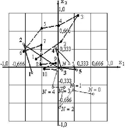
_N.

Example №1. Consider the problem of determining the global minimum of the function [2]:

 

2 ₁ ₁

2 2

1

x

cos

18 x

cos

18 x

x

F

X







(23)



1 

x

₁

;

x

₂



1

(24) and explore on it the search properties of algorithms described above.

The function (23) in (24) has 25 local minima and 10

gullies, the global minimum

X

*



0 ,

0

.

The adduced above algorithms of random search type smoothing [7] in the integral form adapted for storage and use of previous experience, i.e. have the property of adaptation. In particular, the algorithm 2 has four parameters

d

₁

,

d

₂

,

k

₁

,

k

₂ defining the probabilistic properties of directions and selecting the length of trial step. For each set of parameters, for a certain starting

point

X

0 and a priori given the lower limit of the norm of vector



_N

:



_N





we define the loss function:

 



₁

,

₂

,

₁

,

₂

,

X

0

,

Ω





₃ _

 

Ω



₄



X

**

 

Ω



X

*







,

U

d

k

N

k

(25

)

where:

N

_

 



 the number of trial points needed to

reach the point

X

_N



X

**at which



_N





;



 is a set of random numbers, with help of which was

0 



 the necessary search accuracy;

k

₃



0 ;

k

₄



0 ;

 weighted coefficients which establish the equivalence of sampling points, which are calculated to further reduce the

difference

X

**



X

*





on per unit (

k

₄



0

if







* * *

X

).

As the experience of numerical experiments, the value of the function (25), quite strongly depends on the sequence  and the starting point for a fixed set

2 1 2 1

,

d

,

k

,

k

(8)

International Journal of Emerging Technology and Advanced Engineering

86

Therefore, as the objective function for the problem of choice of rational parameters of training we use



d

₁

,

d

₂

,

k

₁

,

k

₂



M

_, 0





d

₁

,

d

₂

,

k

₁

,

k

₂





X

U



_ .

Then the problem of choosing the optimal training parameters for the considered object (23), (24) can be reduced to a mathematical programming problem: find a minimum of the function



d

₁

,

d

₂

,

k

₁

,

k

₂



U

(26)

with restrictions:

.

2 ,

1 ;

;







  



i

k

d

_i _i _i _i _i _i (27)

To solve this problem was used algorithm №1. The search process took place at such initial data:

;

1 ,

0 ;

4 ,

0 ;

2 ,

0 ;

10 ;

10

3



2 ₁



₂



₁



    

k

d





.

10 ;

5 ;

1 ,

0

₁ ₂ ₃ 2 ₄

2



 

 

k

d

k

for

X

**



X

*



10

2

For each set

d

₁

,

d

₂

,

k

₁

,

k

₂ the search

X

**



X

 0

,





has began out of five different starting points, evenly distributed along the constraints (24). At this with the purpose of obtaining the averaging over the random number sequence, this procedure was repeated 10 times for each of the starting point. As a result were found

these parameters:

47 ,

0 ;

79 ,

1 ;

38 ,

0 ;

976 ,

0

₂ ₁ ₂

1



d



k



k



d

.

Using the procedure described above were chosen the same settings for ASE algorithm for object (1.23)−(1.24). The numerical values of the parameters were respectively ASE:

83 ,

0 ;

91 ,

0 ;

621 ,

0 ;

753 ,

0

₂ ₁ ₂

1



d



k



k



d

With these sets of parameters for the algorithm №2 was obtained

X

**for 290 trial points on average (standard middle-quadratic deviation was 93 trials

ASE − 320 (standard middle-quadratic deviation − trials).

The equivalence of the losses on the search for algorithms is not accidental and is explained by a certain

similarity of density distributions



_N

 

Ξ

, as well as sufficiently close values of the factors of forgetting the prehistory of search.

Example №2. The choice of rational parameters of learning of algorithm №2 for gullied function is carried by the example of the optimization of function

 



 

₂



2

2 1 2

1 2 2

1















x

F

X

at different

values



₁

,



₂

,



, which respectively define the steepness of the walls of the ravine, the measure of non-linearity the lines of level of the bottom of and the

degree of reduction of curvature

f

 

X

near the line

2 1 2

2

x





. Calculations were performed for

5

1 ,

0 ;

1000

10 



₁





₂



with





2

and

4 



.

In the result of studies on the rational minimize of losses were found the intervals of parameters of the algorithm №2 for the function with gullied lines of level:

;

8 ,

1

5 ,

1 ;

965 ,

0

95 ,

0 

d

₁



d

₂



(28)

7 ,

0

55 ,

0 ;

7 ,

2

2 

k

₁



k

₂



(29) The losses on the search practically did not depend on

the parameter



, and for

3

5 ,

0 ;

1000

100 



₁





₂



are accounted for -500 computing of function. When



₁

,



₂



0 ,

5

or



₂



4 ,

5

the losses decreased and, for example, accounted for



₁



10 ;



₂



0 ,

1

-120 trials. With an increase the losses on the search also decreased, as the approach of the branches of the parabola

2 1 2 2

x





the search has "jumped" from one branch to another without moving along the bottom of the ravine.

Example №3. The influence of parameters (28), (29) on the quick of action of the algorithm №2 is investigated by the example of the following mathematical programming problem:

 



100 

x

₁



x

₁2



2





1 

x

₁



2



90 

x

₄



x

₃2



2





1 

x

₃



2



10 ,

1 



x

₂



1  

2



x

₄



1 

2





19 ,

8 

x

₂



1 



F

X



₄



1 



min;



10 



10 ,





1 ,

4 

.

(9)

International Journal of Emerging Technology and Advanced Engineering

87

The condition of stop has been selected

 

2

10





X

F

In calculations, performed without using of intervals (28), (29) at different sets of parameters

2 1 2 1

,

d

,

k

,

k

d

, the averaged losses on the search made up 13000-18000 trials and at set of parameters with account (28), (29) the averaged losses on the search made up

5000-Analyzing the results, we can draw the following conclusions:

1.Displaying the normal distribution of the law of random trials on the entire range of variation of the control parameters increases the reliability of the search at each step.

2.The using of the basis with rotating axes was allowed to construct an algorithm independent global search, designed to optimize the gullied-type functions with local extremes, lying at the bottom of the gully curved form.

3.Introduction of the operation of preliminary settings of gullied algorithm on the test function improves the probability properties of the selection of a successful direction, and the length of the working steps and thus increases the speed of search.

V. GLOBAL SEARCH ALGORITHM "WITH THE RETURN

AFTER AFAILED STEP"

This algorithm has been suggested by the authors of article [14].

n-dimensional Euclidean space

E

_n in some domain given a continuous function

F

 

X



F



x

₁

,

x

₂

,....,

x

_n



, i.e.



n



E

Q



X



.

Is considered the solution of the nonlinear programming problem: find the extreme of function

F

 

X



min,

X



Q

(30) at the performance of restrictions:

 

0 ,



1

1 ,

2 ,....,

1



1

k

m

g

_k

X



(31)

 

0 ,



2

1 ,

2 ,....,

1



2

k

m

g

_k

X



(32)

Consider a modification of the algorithm of random search "with the return after a failed step" [2 − the randomized algorithm with "double return", which can be represented as follows [14]:

 

i

 

i

i i

i

i i

i i i

F

X





















 



 

1

1 1

1

1 1

~

if

~

(33)

Where:

X



_i_₁



X

~

_i



H

_i

Ξ;

X



_i_₁



X

~

_i



2 H

_i

Ξ

 s are distributed

uniformly over the unit

n

 dimentional hyper-sphere;



h

₁

,

h

₂

,...,

h

_m

,



H





The algorithm consists of two sub-algorithms. Sub-algorithm №1 chooses the starting point and sub-algorithm №2 finds the solving of problem.

Sub-algorithm №1. Selection of the starting point. The difficulty of solving the problem (70) for a sufficiently complex constraints (31) and (32) significantly is increased due to the need to "manual" selection of the initial (starting) point belonging to the permissible area.

In [14] it is proposed automatic selection of the starting point of the search process using the following procedure. In the region

Q

, which belongs to the space

n

E

, randomly selected the starting point, which generally does not satisfy the constraints (31) and (32). Out of this point as center, is constructed hyper-sphere of

predetermined radius

_R

m0_.

After that, by using the pseudorandom numbers -dimensional realization of random vector

 



     



,

,...,

,

₂1 1

1 1 1

in i

i





Ξ

and in the area

Q



E

n

is determined the random point:

 m i

i

X

Ξ

R

X

_₁





;

R

_i m





r

_i₁   m

,

r

_i₂m

,....,

r

_in m



(34) If the point

X

_i_₁ satisfies the constraints (31) and (32), this point is accepted as the starting point; otherwise are performed consistently all the given S realizations of the random vector

Ξ

 _i2

,....,

Ξ

 _iS with the calculation of the formula (34), and is checked constraints (31) and (32). If all the attempts of

S

have not been successful, then the "contraction" of the hyper-sphere radius by the formula



0 ,

1 ,

2 ,...



,

1

_R

_K

(10)

International Journal of Emerging Technology and Advanced Engineering

88 K

 contraction coefficient, which is selected depending on the complexity of constrains and the sizes of the search area for each of the variables (usually ranges from 0.8 to 0.98). Likewise, is selected the number of tests:

S

= (1030). Thereafter is performed a new series of tests of the random point on the surface of the new hyper-sphere. If during the search

starting point

R

mj



R

mj1



K

_R

(

K

_R  criterion values hyper-sphere radius), then the process of variation of hyper-sphere radius stops. Then, according to the formula

_R

mJ1



_R

mJ

_K

,



0 ,

1 ,

2 ,....,

_t



1 

₍₃₆₎ is constructed a new sequence of hyper-spheres. Each time at the changing of the radius are performed the calculations according to the formula (34) with check of constraints (31) and (32). If in the process of construction of i - j hyper-sphere has not been determined the starting point of satisfying the given restrictions, then out of the

last of

S

i

-hyper-sphere, is done the "big step" in a random direction, i.e.



k

q



L

R

m0



mt



k

_,



₀

_,

₁

_,

₂

_,...,

_.₍₃₇₎

The resulting random point is the center of the creation of a new hyper-sphere and a new cycle of the search of starting point. If there is a restriction only of the type (31), the system changes the choice of starting point: at first by program way is formed the auxiliary objective function in the form

 

X



 

X



1

1 1

1 2

m

k k

f

F

, (38)

and then is performed the search of the starting point, i.e. minimum of the function (38), and is performed sub-algorithm №2.

Sub-algorithm №2. Solution of non-linear programming problem. The work of sub-algorithm №2 starts after finding the starting point. Out of it in a random direction are performed successively the series of S of test steps, the length and the number of which is selected depending on the complexity of the objective function and constraints: the more considerable is their nonlinearity, the greater is selected the value of initial step, which is called the "small step".

The first from series of steps leading to a decrease in the objective function is called the "working step", and thus obtained was a point taken as the new starting point (34). If neither step in the series of random sampling is not successful, then there is variation in the length of a "small step" towards its reduction:

   

K

H

_ij1



_ij (39)

where

i



1 ,

2 ,...

 the number of working step;

1 ,...,

,

2 ,

1 



S

j



m

i

k

H



(

k

_m "criterion of the length of "small step") or

F



X

_i_₁

  



F

X

_i





(



 specified accuracy), then out of the point

X

_i_₁ is performed the "big step" in a random direction:

Ξ

X

ˆ

₀



_i_₁



L

, (40)



l

n



L



₁

,

₂

,....,

 the value of this step. At this the length

L

is selected so as to re-cover approximately 3/4 of the area:

B

X

A



, (41) Where

A

and

B



constraints imposed on the control parameters (vector

X

).

In the absence of the condition (41), the length of the "big step" is defined arbitrarily. Obtained in this way

point

X

 0



Q

is checked whether it belongs to the permissible region. The production of a certain number of random tests at failed "small step" in both directions allows a retrieval system, while keeping the same step, rise up the slope, and thus overcome the mountain ranges of the objective function. Consequently, the search itself thus gains global properties. In practice, there is a situation when the function (30) is multi-extreme and the restrictions (31) and (32) are complicated. To overcome this type of obstacles the sub-algorithm №2 includes addition, based on the use of (41). This allows in case of hit of the search system in any of local extremes get out in another zone using the "big step".

In order to evaluate the effectiveness of the algorithm it was conducted numerical experiment on a computer. The task of mathematical programming if formulated as follows: find