Determination of Soil Deformations under Short-Term Dynamic Loading

(1)

International Journal of Emerging Technology and Advanced Engineering

Website: www.ijetae.com (ISSN 2250-2459, ISO 9001:2008 Certified Journal, Volume 9, Issue 4, April 2019)

15

Determination of Soil Deformations under Short-Term Dynamic

Loading

Olga Markova

1

, Helena Kovtun

2

, Victor Maliy

3

1,2,3

Institute of Technical Mechanics of the National Academy of Sciences of Ukraine

Abstract— Determination of soil deformations under loading is an important problem when different tasks are solved. But not enough attention is paid to the problem solution of the total and elastic soil set determination under action of the short-term dynamic loading till now. The aim of the work is to develop a soil deformation mathematical model, which from one side is simplified enough, and from the other side allows determining total and residual deformations of the soil under short-term dynamic loading acting on its surface. The possibility to apply the proposed model to determine the multilayer soil deformations is shown. Results of a test problem solution are given.

Keywords—Soil deformation, short-term loading, elastic-viscose-plastic medium, multilayer soil.

I. INTRODUCTION

There are a lot of real-world problems connected with the soil stability and elasticity under the action of short-term loading. Soil deformations under the external forces action are considered in the elasticity theory problems [1-4]. Soil deformability depends both on its structural connections resistivity and elasticity, and on separate soil components deformability.

If the load acts for one time only, the onetime process of soil loading and unloading has place. In the case when the load is higher than the soil structural strength both elastic and residual deformations are appeared; in some cases residual deformations can be many times larger than the elastic deformations. To calculate soil stress-strain state a finite difference method [1] or a finite elements method [2] can be used, but their application is rather labor-intensive. Besides, the determination of numerical values for many soil parameters necessary for such calculations is a complicated problem, as soil actual features depend on the diversity of factors, which are not studies well (weather, humidity, consolidation degree, etc.). Because of this, it is useful to develop soil deformation mathematical model, which is rather simple from one side, but from the other side gives possibility to determine total and residual soil deformations under short-term dynamic loading acting on the surface with the accuracy enough for the practical problems solution.

Solution of problems connected with the short-term loading action to the soil is based on some model conceptions of continuum features under the loading. The more general principles of soil action models development are given by L. Sedov and G. Lyakhov [3].

II. METHOD

One of the approaches is the substitution of the actual ―loading – deformable semispace‖ system by the idealized mechanical system, which parameters correspond to the soil physical-mechanical properties [5, 6]. In this case the combination of actual soil rheological features can be performed as the combination of elemental bodies’ features. In rheology the elemental bodies are the Hookean elastic body amendable to the equation of state E ( is the stress, E is the elasticity module,  is the deformation); Newtonian liquid amendable the equation of state  ( is the viscosity coefficient,  is the deformation change speed); Saint-Venant’s rigid-plastic body working in accordance with the dry friction low with the _s amplitude value (_s is the working stress in the soil). The elemental bodies reflecting real soil simple features (elasticity, viscosity, and plasticity) can be performed by the mechanical models as a spring and dampers of viscose and dry friction respectively. The variation of the acting stresses in time is determined by the ratio of the applied dynamic load value to the distribution area.

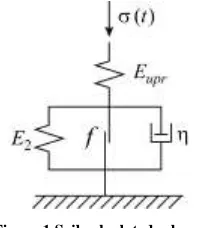
The analysis of different soil calculated schemes and rheological models has shown the appropriateness to use a mechanical system with one degree of freedom, which motion is determined by the rheological model of the elastic-viscose-plastic continuum without inertia, as a soil calculated scheme to determine total and residual soil deformations under the short-term loading action. In this calculated scheme the element with parallel located spring with the elasticity module E₂, damper with viscosity , and dry friction element with coefficient f are placed in

series with the spring with the elasticity module E_upr(see

(2)

International Journal of Emerging Technology and Advanced Engineering

Website: www.ijetae.com (ISSN 2250-2459, ISO 9001:2008 Certified Journal, Volume 9, Issue 4, April 2019)

16

The considered element works as follows. At the time

0



t the pressure developing the stress (t), is applied. It is growing till the determined value _m, and after it is reducing till zero or growing again at some time interval. Here only the spring E_upr is deforming till (t)_s. At

s t 

() the continuum viscose-plastic features appear and the spring E₂ and viscose friction damper begin to work.

At the loading reduction up to _s the partial unloading of

springs E_upr and E₂ takes place because of the viscose

friction damper delay, and at (t)_s the spring Eupr is

totally unloaded, and at this the spring E_upr elastic module

[image:2.612.118.218.331.445.2]

may be different at loading and unloading. So, when the stress is removed the residual deformations occur.

Figure 1 Soil calculated scheme

III. CALCULATION

Mathematical description of the considered model consists of the set of equations; each describes the specific continuum state. These equations are used sequentially in dependence on the applied load value and its action regime. Such model can be used to continuum in which the limiting compression-test and unloading diagrams can be considered as linear ones; and residual deformation values are essential in comparison with the elastic deformation values.

Let’s mark diagrams of dynamic (at the stress speed

 

 and deformation speed change ) and static (at 0 and 0) continuum compression by:

    

 Eupr ; Edef , (1)

where 1/E_def 1/E_upr1/E₂.

Continuum deformation is equal to

2 1  

 , (2)

where ₁ is connected with the instantaneous

compression, and ₂ is connected with the compression in time.

At the stress growing the equation determining the continuum behavior coincides with the equations of the linear viscous-elastic continuum:

upr E / 1  

 at (t)_s; (3)

), (

/ ,

/

/E_upr  E_def E_uprE_def  E_uprE_def       

at (t)_s, (4)

Where  is the viscosity parameter,  is the viscosity coefficient.

At the loading reduction the spring E_upr is releasing,

and the spring E₂ is still compressing. In this case the equation describing the continuum behavior is as follows:

at (t)_s

), / 1 / 1 ( ) / 1 / 1 / 1 ( / raz upr m raz upr def raz E E E E E E               (5)

where E_raz is the elasticity module of the first spring at

releasing; _m is the maximum stress at which the release begins.

Equation (5) stops to be valid when the second spring deformation approaches its maximum value (₂0). At further stress reduction the second spring deformation is taken as the invariable one. The equation describing the continuum behavior is as follows:

at (t)_s

s raz s E 

     

 ₁ ( )/ , (6)

Where _s is the deformation value at (t)_s during the release.

The continuum behavior is determined by the set of equations (3 – 6), changing at the deformation process.

At the repeated loading growing the model works as follows. If the secondary loading is at the moment when equation (5) is valid, this equation action is kept till the stress is equal to _m, from which the release has begun.

(3)

International Journal of Emerging Technology and Advanced Engineering

Website: www.ijetae.com (ISSN 2250-2459, ISO 9001:2008 Certified Journal, Volume 9, Issue 4, April 2019)

17

If the loading begins to grow when equation (6) is valid, it is acting further till the stress has its maximum value _s, from which the release begins. At the further stress growing equation (5) is valid, and when the stress is equal to _m, from which the stress release has begun, equation (4) is valid.

The described model of the elastic-viscous-plastic continuum can be used to calculate total and residual deformations not only for the case of one layer soil, but also for the multilayer soil under the short-term loading. In this case the set is determined as the compression of the soil column, which consists of the layers with different features. The total set is determined as the sum of each layer deformation; for each layer the deformation module is constant.

Here each layer is modelled by the elastic-viscous-plastic element, which characteristics correspond to the physical-mechanical properties of the given soil layer, and the load acting to the upper and lower layer bounds depends on its depth of occurrence. Deformations for the layer bounds can be determined by the set of equations (3 – 6), and the total deformation for the multiple layers can be calculated by the layerwise summation method for the sets of each layer inside the limits of the compressible soil column [7].

To calculate stresses in the soil column the formula of the maximum compressing stresses distribution along the depth under the center of the loaded area [8]

), ( ) (

max_x t k₀ t (7)

where max_x(t) is the maximum compressing stress in

the soil at the depth x; k₀ is the tabulated coefficient;

) (t

 is the intensity of the uniform load.

As the result of the joint resolution of equations (3 – 6) we have instantaneous values of relative deformations of the multilayer soil bounds at each integration step. The deformation for each soil layer with the soil thickness h_i

can be determined in accordance with the relative deformations of the upper ( j=1) and bottom ( j=2)

bounds of the i-th layer at each time moment as follows:



  

 2

1 *

2 _j j

i i

h

. (8)

The total soil deformation at each time moment is determined as the sum of each layer deformations:



  

 n

i i 1

*_, ₍₉₎

where n is the number of soil levels.

Soil deformation after the stress removal is the residual deformation _o of the soil area. Knowing the total  and

residual _o deformations of the soil area, one can determine the elastic deformation for the full load action period:

o upr 

 , (10)

where  is the total soil deformation for the full load action period.

When it is necessary one can determine total, elastic and residual deformations for each layer of the soil area.

Using the described approach for calculations it is necessary to take into account the fact, that residual deformations at some depth of the soil column may not occur, they occur only for the depth where the condition

s t 

() is valid.

With the use of the approach described the algorithm and computer software have been developed to calculate total and residual deformations under the action of short-term loading.

IV. RESULTS

As an example the results of soil set calculation of the three layer soil with different characteristics are given. The initial data for calculations is:

 n is the number of soil layers;

 Eupri is the soil elasticity module for the i-th layer;  Edefi is the soil deformation module for the i-th layer;  E_razi is the soil release module for the i-th layer;

 S is the area of load distribution;

 h_i is the i-th layer thickness;

 _i is the viscosity parameter for the i-th layer;

 _si is the permissible stress in the soil for the i-th layer;

 k_oi is the tabulated coefficient to calculate stress in the soil point at the given depth.

(4)

International Journal of Emerging Technology and Advanced Engineering

Website: www.ijetae.com (ISSN 2250-2459, ISO 9001:2008 Certified Journal, Volume 9, Issue 4, April 2019)

18

Figure 2 Dependence of the force acting on the circle area on time

Elastic and viscous-plastic deformation modules and viscosity coefficients for each soil layer are taken from the books [9, 10].

The considered soil consists of three layers: dry sand, loam, and seasonal frozen soil. Its characteristics are as follows:

– the upper layer is the dry sand with the thickness h₁=1 m, k_o₁=0.246; Eupr=200 MPa;

def

E =30 MPa; E_raz=400 MPa; =500 s-1; _s=0.30 MPa; – the middle layer is the loam with the thickness

2

h =1 m, k_o₂=0.0073; E_upr=30 MPa; E_def =5 MPa;

raz

E =60 MPa; =350 s-1; _s=0.10 MPa;

– the bottom layer is the seasonal frozen soil with the thickness h₂=5 m, k_o₂=0.011; E_upr=9000 MPa;

def

E =9000 MPa; E_raz=9000 MPa; =500 s-1;

s

 =3.50 MPa.

As the calculations results first the total , elastic _upr, and residual _o deformations for each soil layer are determined.

The obtained dependencies of the dry sand, loam and seasonal frozen layer deformations on the stress acting to the soil are shown in Figs. 3, 4 and 5. Numerical values of the sets obtained are the follows:

– For the first soil layer (dry sand):



 17.1 mm; _upr=11.3 mm; _o=5.8 mm; – for the second soil layer (loam):



 25.5 mm; _upr=15.5 mm; _o=10.0 mm; – for the third soil layer (seasonal frozen soil):



 0.023 mm; upr=0.022 mm; o=0.001 mm.

Then with the layerwise summation method use the total, elastic and residual deformations of the considered soil area are determined. These deformations are equal to:



 42.6 mm; _upr=26.8 mm; _o=15.8 mm.

[image:4.612.355.533.384.478.2]

Figure 3 Stress () for the first layer (dry sand) of the three layer soil

Figure 4 Stress () for the second layer (loam) of the three layer soil

Figure 5 Stress () for the third layer (seasonal frozen soil) of the three layer soil

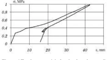
[image:4.612.356.531.544.642.2]

The dependence of the three layer soil total set on the acting to its surface stress is given in Fig. 6.

Figure 6 Total stress () for the three layer soil

(5)

International Journal of Emerging Technology and Advanced Engineering

Website: www.ijetae.com (ISSN 2250-2459, ISO 9001:2008 Certified Journal, Volume 9, Issue 4, April 2019)

19

V. CONCLUSION

The proposed mathematical model allows estimating total, elastic and residual deformations occurring in complicated composition soil under the action of the short-term forces.

REFERENCES

[1] Verigo, M.F., 1988. An approach to calculate subgrade deformation under the action of the dynamic forces. Vestnik VNIIZHT. 5, 4-45. (in Russian).

[2] Liakhov, G.М., 1974. Basis of the explosion waves dynamics in soil and rocks. Nedra, Мoscow. (in Russian).

[3] Unsaturated Soil Mechanics – from Theory to Practice – Chen et al. (Eds), 2016. Taylor & Francis Group, London. ISBN 978-1-138-02921-7.

[4] Kafle, B., Wuttke, F., 2015. Soil Behavior under Unsaturated and Long term Vertical Cyclic Loading. Deformation Characteristics of Geomaterials, V. A. Rinaldi et al. (Eds.). Proceedings of the 6th International Symposium on Deformation Characteristics of Geomaterials, IS-Buenos Aires, IOS Press. P.890 897. ISBN 978-1-61499-601-9.

[5] Liakhov, G.М., 1982. Waves in soil and porous multicomponent mediums. Nauka, Мoscow. (in Russian).

[6] Kovtun, H.N., Krivoviaziuk, Yu.P., Markova, O.M., 1992. Soil mathematical model under the short-term loading. Dynamics and control of the mechanical system motion, Naukova Dumka, p.52-57. (in Russian).

[7] Pjankov, S.А., Azizov, Z.K., 2008. Soil mechanics. Uljanovsk state technical university, Uljanovsk. (in Russian).

[8] Tsytovich, N.А., 1979. Soil mechanics. Vysshaja shkola, Мoscow. (in Russian).

[9] Kharkhuta, N.Ya., Vasiliev, Yu.M., 1975. Strength, stability and consolidation of the road subground. Transport, Мoscow. (in Russian).

[10] Trofimov, V.Т., at al., 2005. Pedology. МGU, Мoscow. (in Russian).