Munich Personal RePEc Archive
Paying for prominence
Armstrong, Mark and Zhou, Jidong
University College London (UCL)
27 April 2011
Paying for Prominence
Mark Armstrong
University College London
Jidong Zhou
University College London
April 2011
Abstract
We investigate three ways in which …rms can become “prominent” and thereby in‡uence the order in which consumers consider options. First, …rms can a¤ect
an intermediary’s sales e¤orts by means of commission payments. When …rms pay commission to a salesman, the salesman promotes the product with the highest
com-mission, and steers ignorant consumers towards the more expensive product. Second, sellers can advertise prices on a price comparison website, so that consumers
inves-tigate the suitability of products in order of increasing price. In such a market, equilibrium prices are lower when search costs are higher since a …rm’s bene…t from being investigated …rst increases with search costs. Finally, consumers might …rst
consider their existing supplier when they purchase a new product, which suggests a relatively benign rationale for the prevalence of cross-selling in markets such as retail
banking.
Keywords: Consumer search, e-commerce, price comparison websites, cross-selling,
mis-selling, commission sales.
1
Introduction
In many markets, consumers are initially imperfectly informed about the deals available, and must invest e¤ort to …nd out where to obtain a reasonable product at a reasonable price. In a few situations it makes sense to suppose that consumers search randomly
through available options. In many circumstances, however, consumers consider options in a non-random manner, and might choose …rst to investigate those sellers or products which have high brand recognition, which are recommended by an intermediary, which are prominently displayed inside a retail environment, which are known to have a low price, or from which the consumer has purchased previously.
In Armstrong, Vickers, and Zhou (2009) and Zhou (2011), we examined how a …rm’s pro…ts and its incentive to choose its price depend on whether it is “prominent” in a consumer’s search process or not. Armstronget al. (2009) considered a situation in which one …rm is sampled …rst by all consumers, and then the remaining …rms are sampled randomly, while Zhou (2011) considered the case where …rms were sampled in a known, deterministic order. We used a search model with di¤erentiated products which was …rst developed by Wolinsky (1986). In this framework, a prominent …rm’s pro…t is greater, although its price is lower, than that of its harder-to-…nd rivals.
Other work, including Arbatskaya (2007), Armstrong et al. (2009, section 4) and Xu, Chen, and Whinston (2011), examined the impact of prominence when …rms supply a homogenous product, but where consumers di¤er in their cost of search. In such a setting, expected prices must be lower in less prominent positions—that is to say, a prominent …rm sets a higher price—otherwise a consumer would never invest in costly search to …nd another …rm.1 In this situation, rational consumers must somehow be compelled to search
through the options in the designated order, or they must …nd that sampling the prominent option is su¢ciently less costly than sampling others, for otherwise they would be better o¤ visiting the cheaper, less prominent sellers …rst.
A fundamental issue concerns the source of prominence, and in this paper we examine three ways in which …rms can become prominent in search markets. To this end we study a variety of stylized models of such markets, including markets with homogenous products and with product di¤erentiation. In section 2 we consider a setting where …rms buy prominence by o¤ering …nancial inducements to intermediaries. We consider two variants of this situation. In the …rst, …rms pay sales commissions to a salesman (not conditioned on whether a product is made prominent), as is often the case in one-to-one sales environments such as for …nancial services. The salesman chooses to promote the product with the highest commission, and in equilibrium he steers the less informed consumers towards the more expensive product. This could be construed as a form of “mis-selling”. In the second
1This prediction is veri…ed in McDevitt (2011), who …nds that plumbing …rms whose chosen name
situation sellers compete to o¤er a lump-sum payment to an intermediary, and whichever …rm o¤ers the most is placed in the prominent position. (This might apply to publishers competing to be chosen as the “book of the month” by a bookshop.) Market performance can be improved by the ability of …rms to buy prominence, as the …rm which is willing to pay the most to be promoted is often the …rm which consumers would most like to encounter …rst.
Next, in section 3 we suppose that …rms can advertise their prices, for instance on a price-comparison website. Although consumers need also to investigate a product’s suit-ability, consumers will …rst investigate those suppliers who advertise low prices. Thus, instead of …rms achieving prominence by means of high commissions, …rms here become prominent when they choose low retail prices. In such a market, in contrast to most search markets, higher search costs induce lower equilibrium prices since a …rm’s bene…t from being investigated …rst increases with search costs. Finally, in section 4 we discuss how in some markets it is plausible that consumers exhibit “default bias”, in the sense that people who are already customers of one …rm may …rst consider this …rm when they decide about subsequent products. In the retail banking market, for example, when consumers need products such as a mortgage or insurance policy, they often consider their existing bank …rst. In such cases, an incumbent …rm is prominent in its customers’ future buying decisions. Because prominent …rms enjoy greater pro…ts than less prominent rivals, a …rm will buy prominence by competing aggressively for a customer’s initial purchase.
Of course, there are other routes to prominence. For instance, a taxi …rm can call itself “A1 Taxis” to be listed …rst in an alphabetic directory.2 Advertising is another common
method of achieving prominence. With an advertising campaign …rms can make their product or brand prominent in a consumer’s mind, so that a consumer is more likely to consider that product …rst when she decides what to buy. Bagwell and Ramey (1994) propose a model with homogeneous products in which some consumers choose …rst to investigate the …rm which advertises the most intensively, which is thereby prominent in these consumers’ search decisions. (In their model, advertising contains no information about price or product attributes, but is done purely to in‡uence search behavior.) Owing to assumed scale economies, when a …rm has greater demand it o¤ers a lower price, and therefore it is indeed rational for these consumers to coordinate on the …rm which advertises
2McDevitt (2011) documents how a high proportion of …rms in certain “home emergency” markets
the most. Because a …rm enjoys a discrete jump in demand when it advertises even slightly more than its rivals, in equilibrium …rms choose their advertising intensities according to a mixed strategy. Haan and Moraga Gonzalez (2011) present a related model with product di¤erentiation in which a …rm which advertises more intensively than a rival is more likely (but not certain) to be considered …rst by consumers. Since a …rm’s pro…t increases when a greater proportion of consumers sample it …rst, …rms have an incentive to buy prominence in this way. In their basic symmetric model, all …rms advertise with the same intensity, with the result that consumer search ends up being random and advertising expenditures are pure waste.
A way to pay for prominence which has recently been analyzed extensively, for instance by Chen and He (2006), Edelman, Ostrovsky, and Schwarz (2007), Varian (2007) and Athey and Ellison (2011), concerns sponsored links on search engines. In broad terms the seller which pays the most for a speci…c search term on a search engine will be prominently displayed on the results returned when someone types in that search term. Since internet users often click on prominent links …rst (either because this is their rule of thumb, or because they have learnt that sellers who are prepared to pay the most to be prominent are often the most relevant), it is worthwhile for sellers to pay for prominence in this way. We discuss related issues in more detail in the next section.
2
Paid Promotion
In some markets, intermediaries highlight one product from among the available options which a consumer should consider …rst. Examples include search engines which list some results more prominently, …nancial advisors and other one-to-one sales advisors who choose the order in which they present options to consumers, doctors who recommend a course of medical treatment, stores which put some products on prominent display at eye level or with greater shelf space,3 shopping malls which put a particular store in a prime position,
a motoring magazine which favourably reviews a particular car, or a bookseller promoting its “book of the month”. While the hope is that better or cheaper products will be chosen
3Dreze, Hoch, and Purk (1994) report results from experiments in stores—their own and previous
for special treatment in these ways, a natural worry is that the intermediary will promote an unsuitable or expensive product when paid to do so.4
There are at least two natural formats for the …nancial incentives which sellers provide to the intermediary: (i) the intermediary is paid per sale on a commission basis, regardless of whether the product is prominent or not, and (ii) the incentive takes the form of a lump-sum payment to the intermediary conditioned on the product being made prominent.5
In many cases, especially in a one-to-one sales environment as is common with …nancial services, marketing e¤orts can be hard to monitor and format (i) is more likely to apply. Given the menu of commission rates he is o¤ered, the salesman then decides which product to promote. Note that format (i) can be implemented in a retailing context when a supplier o¤ers its product to a store with a speci…ed wholesale price and a speci…ed retail price. The margin between the retail and the wholesale price is then the “commission” paid to give the store an incentive to favour its product.6 Format (ii) applies best to situations in
which a supplier can monitor the marketing e¤orts of the intermediary (e.g., a publisher knows that its book was indeed the “book of the month”).
We discuss these two cases in turn.
Commission sales. To investigate this …rst situation, we study a variant of Varian
(1980) whereby Varian’s framework is modi…ed to allow the intermediary (or “salesman” for brevity in the following) to steer the uninformed portion of consumers towards a particular product. In more detail, two sellers supply a homogenous product which all consumers value at v. A fraction of consumers costlessly observe the two retail prices o¤ered by the sellers (and buy from the lowest-price seller) and a fraction 1 of consumers only
4Anecdotal evidence suggests that some bookstores “recommend” books before they have even been
read. One UK bookstore was alleged in 2006 to charge publishers £50,000 a week to guarantee a book “a prominent position in the store’s 542 high street shops and inclusion in catalogues and other advertising”. A trade body suggested that 70 per cent of publisher promotional budgets were spent on so-called “below-the-line” schemes operated by bookshops rather than more traditional advertising. For more details, see the article in the (UK)Sunday Times by Robert Winnett and Holly Watt titled “£50,000 to get a book on recommended list”, 28 May 2006.
5In terms of online advertising, which is one of the leading ways to pay for prominence, the …rst form
of payment is akin to per-click charging, where the advertiser pays the search engine each time someone visits the advertiser’s website. The second form is more akin to so-called per-impression charging, where an advertiser pays for the right for (say) a banner advert on a particular website, and pays each time a consumer visits that website.
consider a single product and buy if the retail price of that product is belowv. The salesman has the ability to steer the 1 less informed consumers to buy either of the products. Suppose that a …rm chooses its retail price, p, and commission rate,b, simultaneously (and simultaneously with the rival seller). A …rm pays commissionb to the salesman every time a sale of its product is made. We assume that the salesman has no ability to alter the retail price, for instance by reducing the price below the stipulated price from the seller by contributing a portion of his commission to the consumer. (Later, we discuss the impact of relaxing this assumption.)
First, note that the salesman will choose to promote the high-commission product, regardless of how the two retail prices compare (as long as prices do not exceed v). This is because the salesman’s marketing e¤ort cannot in‡uence the choice of the informed consumers at all, but fully determines the choice made by the uninformed consumers. Hence, the salesman will direct the uninformed consumers towards the product which pays a higher commission rate.
Second, there are no equilibria in which …rms set either a deterministic price or a deterministic commission rate (or both). For instance, if its rival is known to o¤er the deterministic retail price p, then a …rm enjoys a discrete jump in its demand if it slightly undercuts this price since it then sells to all the informed consumers. Likewise, if its rival o¤ers a deterministic commission rate, a …rm has an incentive to pay a slightly higher commission, since then the salesman directs all the uninformed consumers to its product. We therefore look for a (symmetric) mixed-strategy equilibrium. The following prelimi-nary result (proved in the Appendix) shows that in any such equilibrium high commission payments are associated with high retail prices:
Lemma 1 Let [0; v]2 be the support of the joint distribution of (p; b) in a mixed
strategy equilibrium. Then cannot include two pairs(p1; b1)and(p2; b2) withp1 < p2 and
b1 > b2.
In essence, this result indicates that there is a deterministic and increasing relationship between a …rm’s choice of b and p. Since high commissions are associated with high retail prices, the salesman promotes the highly priced product due to the high commission he then receives. This could be interpreted as “mis-selling”, since uninformed consumers are directed to buy the more expensive product.7
The next result characterizes the equilibrium in more detail:
7This model could also apply to sponsored search auctions, where the highest bidder for a particular
Proposition 1 There is a symmetric mixed-strategy equilibrium in which each …rm chooses its retail price p according to c.d.f. G(p) with support [pmin; v], where G( ) satis…es
(1 )[1 G(p)] = 1 1
1 + 1 2 vp 1
(1)
and
pmin = (1 )v ;
and chooses its commission as a deterministic function of its price so thatb =B(p), where
B(p) = 1 (p pmin) : (2)
It is useful to discuss the main ideas involved in the construction of this equilibrium. Suppose that …rm 2 follows the proposed equilibrium strategy. Then, since the salesman promotes the higher-commission product, …rm 1’s expected pro…t if it chooses the pair
(p; b) is
(p; b) = (p b)[(1 ) Pr(~b < b) + Pr(~p > p)]
= (p b) (1 )G B 1(b) + (1 G(p)) : (3)
In equilibrium a …rm will be indi¤erent between all choices(p; B(p))forp2[pmin; v]and for
a givenpin the support, a …rm’s expected pro…t is maximized over all possible commission rates b by choosing b = B(p). Therefore, a …rm’s pro…t must be locally “‡at” in all directions at the point (p; B(p)). In particular, a …rm’s pro…t in (3) must be unchanged (to …rst order) if it increases both p and b equally by some small amount " starting at b=B(p). Since this change has no impact on the …rm’s marginp b, from (3) we require that
d
d" (1 )G B
1(B(p) +") + (1 G(p+"))
"=0 = 0 ;
i.e., that
(1 ) g(p)
B0(p) g(p) = 0
a system is similar to the early system for selling online advertising, as described by Edelmanet al. (2007, pp. 245-246). Since that time, sponsored search positions have usually been allocated with a generalized second-price auction, so that the ith highest bidder for a particular keyword is listed in theith position but pays the(i+ 1)thhighest bid per click. In our simple duopoly model, this corresponds to a situation
so that
B0
(p) 1 for all p2[pmin; v] :
Thus, the commission rate is a linear (a¢ne) function of a …rm’s price.8 When a …rm o¤ers
the lowest possible commission rate b which might be o¤ered in equilibrium, it knows for sure it will not be made prominent by the salesman, in which case it should o¤er no commission at all. We deduce that in equilibrium we must have B(pmin) = 0, and so the
commission schedule is as in (2).
For now, assume that the …rm chooses commission b=B(p)in (2) when it chooses its price p, and consider its incentive to choosep. From (3), its pro…t withp is
1
[(2 1)p+ (1 )pmin] [(1 )G(p) + (1 G(p))] :
Since in equilibrium the price p = v is sometimes chosen, this pro…t must be equal to
1 [(2 1)v + (1 )p
min]. To maintain the …rm’s indi¤erence over price, the c.d.f. G
must satisfy (1), and pmin is then determined from the condition G(pmin) = 0. Note that
G(p) in (1) is increasing in p for pmin p v. One can also check that p b > 0 for
all pmin p v, so that a …rm always obtains a positive margin when it makes a sale.9
It remains to verify (as we do in the Appendix) that a …rm has no unilateral incentive to deviate to(p; b) with b6=B(p).
In this equilibrium, the uninformed consumers are directed to buy the more expensive product. A …rm either serves the uninformed consumers (when it happens to set the higher retail price) or the informed consumers (when it is the cheaper supplier). When is close to 1, so that most consumers are well informed, then neither the …rms nor the salesman can extract signi…cant pro…t. When almost all consumers are uninformed ( 0), retail prices are approximately equal to the monopoly price v, but almost all of this price is extracted by the salesman, who can steer almost all consumers with his marketing e¤orts.
8This linearity is the chief modelling advantage of assuming there are just two sellers. If there were
n >2sellers, the corresponding formula becomes
B0(p) =1 G(p)
1 G(p)
n 2
so that there is a nonlinear relationship between b and p which depends on the (endogenous) form of
G( ). This complicates the analysis considerably compared to this duopoly setting where we can deduce the shape of B(p) without …rst calculating G(p). Note that with more than two …rms, the commission scheduleB(p)is strictly convex inp.
9Note thatp > B(p)if and only if (1 2 )p <(1 )2
v. If 1=2, this inequality surely holds. If
This trade-o¤ can also be seen by noting that a …rm’s equilibrium pro…t is = (1 )v, which reaches its maximum at = 12.
This analysis presumes that the salesman cannot a¤ect a seller’s retail price, and thus there is a form of (minimum) retail price maintenance applied by sellers. Suppose instead that the salesman can reduce the price a consumer pays for a product by contributing a portion of his commission b. In the equilibrium in Proposition 1, does the salesman have an incentive to o¤er such a discount? Suppose the high-price seller chooses (pH; bH) while
the low-price seller chooses (pL; bL), where bi and pi are related by (2). If the salesman
does not alter the retail prices, his expected commission payment is
(1 )bH + bL (4)
as the informed consumers buy the low-price product and the uninformed consumers buy the expensive product. The alternative strategy involves the salesman reducing the retail price of the expensive product (with a high commission) so that all consumers choose to buy it. To do this entails discounting pH by (pH pL) to make it competitive with the
cheaper product. When he does this, his net commission payment from each consumer is
bH (pH pL) :
However, this net commission payment is lower than the payment in (4) he receives when he does not distort retail prices if (bH bL)< pH pL. One can check from (2) that this
must be true. We deduce that in the equilibrium in Proposition 1, the salesman has no incentive to discount either …rm’s retail price, even when he has the ability to do so.
There are at least two natural benchmarks with which to compare the equilibrium outcome when commissions are paid. The …rst benchmark is when there is no salesman, and the uninformed consumers buy randomly from the two …rms. In this case the framework reduces to Varian (1980)’s model. Again, there is no pure strategy equilibrium in prices, and if its rival chooses its price according to c.d.f. G^( ), a …rm’s pro…t when it chooses price p is modi…ed from (3) to be
p 1
2 + (1 G^(p)) :
To maintain the …rm’s indi¤erence over price, this pro…t must always equal 1
2(1 )v, the
pro…t when the …rm sets the highest possible price. Therefore, the c.d.f. for prices with random search is given by
1 G^(p) = 1 2
v
with the lowest possible price being p^min = 11+ v. One can check that G^(p) > G(p) for
^
pmin < p < v, where G is described in (1), and so retail prices are higher, in the sense of
…rst-order stochastic dominance, when …rms pay commissions to a salesman to promote their product relative to the situation with random search. This is due in part to the sales commissions which arti…cially in‡ate the marginal cost of selling a product. However, whether …rms enjoy greater pro…ts when they pay commission is ambiguous. Without commission payments, each …rm makes expected pro…t ^ = 12(1 )v, while in the regime with commissions a …rm makes expected pro…t = (1 )v. Thus, more pro…t is obtained with commission payments when > 12, so that the uninformed consumers are in the minority. But when the uninformed consumers are in the majority, the two …rms end up playing a prisoner’s dilemma due to the …erce competition to become prominent.
0.0 0.1 0.2 0.3 0.4 0.5 0.6 0.7 0.8 0.9 1.0 0.0
0.1 0.2 0.3 0.4 0.5 0.6 0.7 0.8 0.9 1.0
[image:11.595.144.460.317.514.2]lambda
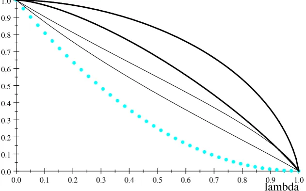
Figure 1: Expected prices and commissions
Figure 1 plots the expected prices paid in these two regimes as a function of , the proportion of informed consumers. (Here,v = 1.) The two bold lines depict expected prices when commissions are paid, where the upper of these lines is the expected price paid by the uninformed and the lower line is the expected price paid by the informed consumers.10
The dotted line represents the expected commission paid to the salesman.11 The two feint
10When commission is paid, the expected price paid by an uninformed consumer is the expected value
of the maximum of two i.i.d. draws from the c.d.f. in (1), while the expected price paid by an informed consumer is the expected value of the minimum of two such draws.
11This is simply the commission payment in (2) evaluated at the expected price paid by all consumers,
lines depict the corresponding prices in the Varian model where no commissions are paid and search is random.12 The two regimes have the same outcome for consumers when
= 0 (when the monopoly price p = v is chosen for sure) and when = 1 (when the competitive price p= 0 is chosen). However, for intermediate values of , the prices paid in the commission regime are substantially higher than when no commissions are paid. Indeed, in most cases an uninformed consumer in the no-commission regime pays a lower price than even the informed consumers do in the commission regime.
The second benchmark with which to compare the outcome with commission payments is to suppose that the salesman is necessary for consumers to buy the product (unlike Varian’s model with random search), but now the salesman is paid by consumers rather than by sellers.13 Suppose that when the salesman is paid by consumers, say in the form of
a lump-sum consultation fee, he directs the uninformed consumers to the cheaper product. (This might be because, all else equal, he has a small intrinsic preference for selling the correct product to consumers.) In this case, all consumers buy the cheaper product and in Bertrand fashion the two sellers are forced to set retail prices equal to cost (zero in this case). The outcome for consumers then depends on how much they have to pay the salesman for his advice. One assumption is that the consultation fee is set equal to the revenue the salesman received under the commission regime, so that the salesman is indi¤erent between the two regimes, perhaps because the advice industry needs to be supportive of a policy shift from a commission-based model to a consumer-fee model. In this case, the expected total price (the price for the product plus the fee to the salesman) paid by any consumer is simply the dotted line on Figure 1. From the …gure it follows that all consumers are better o¤ when they pay the salesman compared to when sellers pay the salesman. In fact, they are also better o¤ when they pay the salesman than when they search randomly (where prices are the feint lines on the …gure).
This section has described a model where …rms attempt to in‡uence a salesman’s mar-keting e¤orts by means of commission payments. The salesman gives prominence to the product which pays the highest commission, and in equilibrium this entails steering
unin-12The expected price paid by the informed consumers is again the expected value of the minimum of
two prices, but this time taken from the c.d.f. in (5), while the expected price paid by the uninformed consumers is just the expected value of one price draw from the same distribution.
13The UK regulator, the Financial Services Authority, published rules in March 2010 concerning how
formed consumers towards the more expensive product. The outcome for consumers, both informed and uninformed, is poor: worse than the situation without commission payments where the uninformed shop randomly, and far worse than a situation in which consumers pay directly for advice.14
Lump-sum payment for prominence. Consider next the case where the …nancial
inducement for prominence is a lump-sum payment, conditional on whether the product is promoted or not. In more detail, suppose that there are two symmetric …rms, and an intermediary auctions o¤ the right to the prominent position. The highest bidder obtains the prominent position and pays its bid, while the loser pays nothing. Once the prominent position is awarded, the two …rms then choose their retail prices. (In contrast to the commission sales case, here it is often natural to assume that …rms observe who has won the prominent position before setting their prices.) Suppose that when …rms choose their equilibrium prices, the prominent …rm makes pro…t H (excluding the lump-sum payment
to the intermediary), while the less-prominent …rm makes pro…t L< H. Given that the
prize of prominence is awarded to a single …rm, each …rm is willing to pay up to H L
for the right to be prominent. The result of the auction is that both …rms bid up to this amount, and the prize is awarded at random to one …rm, who is then made prominent. Since the prominent …rm has paid a lump-sum fee equal to H L, the net pro…t of each
…rm is equal to L. Suppose that 0 is each …rm’s equilibrium pro…t with random search
and L< 0 so that the pro…t of the less-prominent …rm is lower than the …rm would make
in a regime in which consumers search randomly. Then when the intermediary auctions o¤ the right to be prominent the two …rms are forced to play a prisoner’s dilemma and in equilibrium both …rms are worse o¤ relative to the case where no …rm was prominent.15
Whether the intermediary mis-sells the prominent product in this context is ambiguous, and depends in part on whether products are homogenous or di¤erentiated. As discussed
14Inderst and Ottaviani (2010) present an alternative model of potential mis-selling, where the salesman
advises consumers about the suitability of a product rather than its price. There, no consumers are informed, and must rely on the salesman to advise them about which product to buy. The salesman has only a noisy signal about the suitability of a product, and he has an intrinsic preference to recommend the suitable product to a consumer. However, this preference can be overturned if sellers set high enough commissions.
15Armstrong et al. (2009, page 221) show that
L < 0 in their particular model with di¤erentiated
in the introduction, with homogeneous products we expect that the prominent …rm will set a higher price than its rivals, and those consumers with a higher search cost will be directed to buy the more expensive product (as in the previous case with commission sales). By contrast, with di¤erentiated products as in Armstronget al. (2009), we expect that the promoted product is o¤ered at a lower price than the rival product. However, although consumers are guided to the cheaper product …rst, this does not mean that consumer surplus or overall e¢ciency is increased compared to a situation with random search. Armstrong et al. (2009) show in a uniform example that consumers are worse o¤ and welfare declines when one …rm is made prominent. This is because the non-prominent …rms are induced to charge higher prices and the resulted non-uniform prices across …rms lead to less e¢cient match between consumers and products.
Nevertheless, there are a number of situations in which awarding the prominent position to the highest bidder is likely to lead to more e¢cient outcomes, especially when sellers di¤er in the quality or cost of the product they supply. Armstrong et al. (2009, section 3) present a model where …rms di¤er in their quality, and show that the …rm with the highest quality product is willing to pay the most (as a lump sum) to become prominent, and consumers also bene…t when this …rm is placed at the start of their search process. In this model, “prominence” acts as a signal of otherwise unobserved product quality, and this improves market performance. This e¤ect was discussed in a speci…c model in which each …rm had linear demand and “quality” was indexed by the vertical intercept of this demand. However, the result applies much more widely. Indeed, it applies whenever the …rm from a pool of heterogeneous …rms which is prepared to pay the most to become a monopolist is also the monopolist from the pool of …rms which consumers would most like to face.
To see this, suppose there are a large number of heterogeneous …rms in the market, indexed by i = 1;2:::. Speci…cally, suppose the match utility from …rm i is distributed with c.d.f. Fi(u) and that this …rm has constant marginal cost of supply ci. Suppose
in the equilibrium with random search that consumers obtain expected consumer surplus V from participating in the market. Since there are many …rms, each …rm then obtains approximately zero pro…ts. A …rm which is placed in the prominent position and which sets pricepwill sell wheneveru p V, and so makes pro…t i = maxp(p ci)(1 Fi(p+V)),
where pi maximizes this pro…t. (In fact, the …rm will choose this price pi even if it is in a
Expected consumer surplus when …rm i is placed in the prominent position is
vi
Z 1
pi+V
(u pi)dFi(u) +Fi(pi+V))V =V + Z 1
pi+V
(1 Fi(u))du :
In many situations the …rm with the highest i is also the …rm with the highest vi,
so that and v are positively correlated in the population of …rms. To take one simple case, suppose that the only way in which …rms di¤er is in their cost ci, and each …rm
generates the same distribution of match utilities. Then the …rm with the lowest cost is willing to pay most to be in the prominent position, and this …rm also o¤ers the lowest price to consumers. Whenever the highest i and the highest vi coincide, auctioning o¤
the prominent position to the …rm which is willing to pay the most will increase consumer surplus and total welfare, relative to the situation with random search.16;17
3
Price-Directed Search
Price comparison websites are now a major part of the retailing landscape.18 As long as
a consumer has access to the internet, she can almost costlessly gain access to a list of
16Another instance of this situation is seen in the extension of Wolinsky (1986)’s model developed in
Eliaz and Spiegler (2011). Here, a product is suitable with some probability q, which di¤ers across …rms. If a product is suitable, its value is taken from a common distribution, while if the product is unsuitable its value is zero. A …rm’s “quality” q does not a¤ect its pricing decision, and the …rm with the highest
q is willing to pay the most to be prominent, and that is also the …rm which consumers would most like to investigate …rst. Similar e¤ects are also seen in models of sponsored-link auctions, as studied by Athey and Ellison (2011) and Chen and He (2006). There, …rms di¤er in the likelihood of providing a relevant match for a consumer, and an advertiser who is more likely to provide a relevant match is willing to pay more to be listed prominently on the search results page. (There is no e¤ective price competition between advertisers in these papers.) It is therefore rational for consumers to investigate the links in the order presented on the page, as the more relevant links are listed at the top. Again, paying for prominence improves the e¤ectiveness of consumer search.
17Of course, if and v were instead negatively correlated in the population of …rms, then when the
prominent position is sold to the highest bidder, consumers are made worse o¤ relative to the situation with random search. Jerath, Ma, Park, and Srinivasan (2010) consider a model in which a higher quality …rm may prefer to be displayed in a less prominent position than other …rms, once the reduced advertising payments are taken into account. Relatedly, McDevitt (2011) shows that plumbing …rms whose names start with “A” tend to receive a greater number of complaints from consumers, suggesting they are often lower-quality suppliers.
18See Baye, Gatti, Kattuman, and Morgan (2009) and Ellison and Fisher Ellison (2009), and the papers
prices from various suppliers for a wide range of consumer items. Sometimes products may be approximately homogeneous, so that price is mostly what matters for a consumer. In such cases, price comparison websites may go a long way towards achieving competitive outcomes.19 An important early model of a price comparison website with homogenous
products was presented in Baye and Morgan (2001). There, a number of symmetric …rms supply a product, and …rms can advertise their prices on a website to which (in equilibrium) all consumers have access. There are two groups of consumers: some consumers care only about …nding the cheapest supplier, while other “loyal” consumers will only buy from a single …rm to which they have a strong brand preference. The website charges a lump-sum listing fee to sellers, and each seller decides whether or not to put its price on the website. In equilibrium, the decision to advertise on the website is random, and this in turn generates prices which are also random. The …rm which chooses to advertise and which happens to o¤er the lowest price on the website will sell to all the price sensitive consumers, and other …rms will sell only to their pool of loyal consumers.
For some products, however, price is not the only consideration and a consumer cares also about product suitability. For instance, a traveller may look for a ‡ight from London to New York on a travel website, and …nd various ‡ights listed in order of increasing price, but only a subset of the ‡ights meet the traveller’s needs in terms of airport location, departure time, and so on. Nevertheless, price is still an important factor for the consumer, and it is plausible that the consumer will investigate the options in order of increasing price. In these situations, sellers become “prominent” in a consumer’s search process by posting the lowest price on the website.20
In theory, one could try to use the search model with product di¤erentiation in Wolin-sky (1986) to study this question. However, it turns out that this framework, where a consumer’s match utility is independently distributed across …rms, apparently does not
accordingly. An important additional feature in the labour market relative to a typical consumer market is that a job vacancy can be …lled, so that workers do not necessarily visit the highest-wage employer …rst if they anticipate that many other workers will apply for the same post. See Rogersonet al. (2005, section 5) for discussion of these models.
19For the purposes of this discussion, we ignore important caveats to this claim, including the ability that
sellers have to “obfuscate” their true price. For instance, a seller might post a low “price” on the website, but then compensate for this by excessive “postage and packing” charges. See Ellison and Fisher Ellison (2009) for further discussion of this point.
20By contrast, in Armstrong, Vickers, and Zhou (2009) where price information is imperfect, the direction
lead to an easily tractable solution for how …rms choose prices on a price-comparison web-site. Instead, in this section we present a variant of Wolinsky’s model which is tractable, and which provides insight about the impact of price advertising on market performance.
Suppose that two …rms compete to o¤er a di¤erentiated product in a Hotelling frame-work. Speci…cally, the two …rms are located at the ends of the unit interval [0;1], and consumers are uniformly located on this interval, with brand preference parameter de-noted ` 2 [0;1]. The valuation of a consumer at ` for the product supplied by the …rm at 0 is v `t, where v is the valuation of the consumer for the ideal product and t is the unit “transport” cost (not to be confused with the search cost) and captures the extent of product di¤erentiation. Similarly, her valuation for the product supplied by the …rm at 1
isv (1 `)t. (As usual, we suppose v is su¢ciently high that the market is fully covered in equilibrium.) If production cost is normalised to zero, then in the absence of search frictions, so that consumers have full information about their preferred product and the two …rms’ prices, the equilibrium price in this market is p=t.
In the following discussion we introduce search frictions into this market. Speci…cally, we suppose that each consumer must incur a search cost s to visit a …rm to discover its price (where necessary) and its match utility (where necessary), as well as to purchase the product. When a consumer visits the …rst …rm, she discovers her brand preference parameter x, which then also reveals her match utility at the other …rm. Thus, this is a search model where match utilities are negatively correlated across the two …rms, rather than independently distributed as in Wolinsky’s model.
The market without the price comparison website. Suppose that consumers choose
their initial …rm randomly (i.e., they have no idea about their preferred supplier ex ante
and expect …rms to o¤er the same prices). What is the equilibrium price, p , in this market? Consider the incentive of the …rm at 0 to choose its price p. Since consumers anticipate that both …rms choose price p , a consumer who …rst visits this …rm will buy if
p+`t p + (1 `)t+s ;
who end up buying from that …rm is
1 2+
s+p p
2t :
If a consumer visits the rival …rm …rst, since consumers anticipate the price p at both …rms, only those consumers at a distance
` 1
2
s
2t
from the …rm at0 will choose to investigate it. (Note that if s t, then in equilibrium no consumers will search beyond the …rst sampled …rm. To avoid this less interesting case, we assumes < t henceforth.) They will then buy from this …rm unless the price they …nd there is signi…cantly higher than p (i.e., the surprise is big enough to drive some of them back to their initial …rm, which requires thatp > p +s). Thus, at least for local deviations from the equilibrium price p (i.e., for p p +s), the …rm’s total demand is
q = 1 2
1 2+
s+p p
2t +
1 2
1 2
s
2t =
1 2+
p p
4t
which does not depend on s.21 This is like the full information Hotelling model, but with
di¤erentiation parameter 2t instead of t. Therefore, the equilibrium price is
p = 2t :
This price does not depend on the search cost s so long as s >0, and so we see that even tiny search frictions cause equilibrium prices to double. (This is reminiscent of Diamond (1971)’s famous result that arbitrarily small search costs can lead to monopoly prices.) The reason is that a …rm cannot attract more of those consumers who …rst visit its rival with a low price, and so a …rm’s demand elasticity is halved.
The market with the price comparison website. Now suppose that …rms advertise
their prices to all potential consumers (e.g., on a price comparison website). By symmetry, all consumers will …rst investigate the …rm which posts the lower price, and only go on to buy from the second …rm if their discovered brand preference turns out strongly to favour the more expensive product. If the two posted prices are pL and pH > pL, where pH pL< t s, then the low-price …rm has demand
QL =
1 2 +
s+pH pL
2t
21One can check that for a large deviation pricep > p +s, the …rm’s demand isq= 1 2(
1 2+
s+p p
2 ) +
1 2(
1 2+
p p
2t ). That is, the demand function has a kink atp=p +s. But one can show that taking this
and the high-price …rm has demand
QH = 1 QL=
1 2
s+pH pL
2t : (6)
(As before, once a consumer has investigated her …rst seller, she knows the price and the match utility of the second seller. She nevertheless needs to incur the search cost s to buy from the second …rm.) Notice that QL QH =s=t when pL =pH, so that there is a
jump in its demand equal to s=t when one …rm slightly undercuts its rival.22 Due to this
incentive to undercut and the presence of product di¤erentiation, it is clear that there can be no symmetric strategy equilibria. It is also true that there are no asymmetric pure-strategy equilibria either.23 In the following result we derive a (symmetric) mixed-strategy
equilibrium.
Proposition 2 Suppose that 0< s < t. Then the search market with a price comparison website has a symmetric mixed-strategy equilibrium in which each …rm chooses its price according to c.d.f. H(p) with support [pmin; pmax], where H( )satis…es
1 2+
p p
2t + s
2t[1 2H(p)] = p : (7)
Here is a …rm’s expected pro…t in equilibrium and p=Rpmax
pmin pdH(p) is a …rm’s expected
price in equilibrium.
We now describe how to construct this equilibrium and determine the four unknown parameters pmin, pmax, p, and . If its rival chooses price with c.d.f. H, a …rm’s expected
demand when it chooses pricep2[pmin; pmax]is24
Q(p) =
Z p
pmin
1 2
s+p p~
2t dH(~p)
| {z }
demand when rival charges lower price
+
Z pmax
p
1 2 +
s+ ~p p
2t dH(~p)
| {z }
demand when rival charges higher price
22Bayeet al. (2009) …nd in their dataset that a seller’s “click rate” increases by 60 per cent when the
seller lowers its price to become the cheapest seller on the price comparison website. Note that Baye et al. document that a seller’s click rate also depends on its position on the webpage, which re‡ects a second form of prominence.
23To see this, suppose instead that there exists an asymmetric equilibrium withpL< pH. Since @QL @pL = @QH
@pH, the …rst-order conditions implypL=pH =QL=QH. That is, a lower price is associated with a lower
demand, which cannot be the case.
24If instead we adopted Wolinsky’s model with independent match utilities, expected demand does not
= 1 2 +
p p
2t + s
2t[1 2H(p)] : (8) Since the …rm must be indi¤erent between choosing all prices in the interval[pmin; pmax], it
follows that H satis…es (7). (Notice that this calculation of demand assumes that pmax
pmin < t s, and we will check later that this condition is satis…ed in equilibrium.) In
particular, the density for a …rm’s chosen price, h(p), is
h(p) = 1 2s
2t
p2 1 (9)
which decreases over its support.
To complete the equilibrium characterization, we need to determine the four unknown parameters. SinceH(pmin) = 0 and H(pmax) = 1, expression (7) implies that
t+p pmin+s=
2t pmin
(10)
and
t+p pmax s =
2t pmax
: (11)
Given the density h in (9), it follows thatp must satisfy
p= 1
2s Z pmax
pmin
2t
p p dp=
1
2s 2t log pmax
pmin
1 2(p
2
max p2min) : (12)
The …nal condition is derived from the fact that a …rm does not want to set its price higher than pmax. If a …rm chooses p pmax, it will surely be the more expensive …rm, and its
expected pro…t will be
(p) p 1
2
s+p p
2t :
To ensure that the …rm has no incentive to do this, we require that (p) (pmax) for all
p pmax. Since (p)is a concave function, this requires
pmax
1
2(t+p s) : (13)
On the other hand, given the other …rm’s equilibrium strategy, a …rm’s expected pro…t is constant forp2[pmin; pmax], so its derivative with respect to pevaluated atpmax(from the
left-hand side) is zero, which from (8) implies
lim
p!pmax
Q(p) +pQ0
(p) = 0) 1
2(t+p s) pmax=spmaxh(pmax): (14)
From (13) and (14), we conclude that
and
pmax =
1
2(t+p s) =
p
2t : (15)
(The second equality in (15) used (11).) The four unknowns pmin, pmax,p and can then
be solved from (10), (12) and the two equalities in (15).25 In the Appendix, we show that
this system does have a unique solution, and the requirement 0 < pmax pmin < t s is
satis…ed.
An interesting observation (proved in the Appendix) is that a higher search cost induces …rms to post lower prices and so causes equilibrium pro…ts to fall.
Corollary 1 In the equilibrium characterized in Proposition 2, (i) pmin, pmax,p and all
decrease withs, and (ii)pmax < tso that …rms earn less than in the case with random search
without the price comparison website and in the case with perfect consumer information.
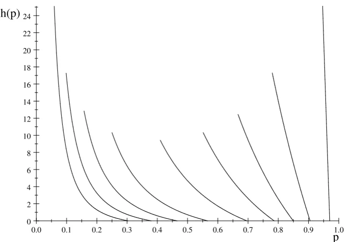
Intuitively, a higher search cost implies that consumers are more reluctant to search beyond the …rst …rm they encounter, so there is a greater bene…t to being the …rm sampled …rst, and hence a greater incentive to be the …rm with the lower price. To illustrate this feature, Figure 2 depicts the density h( ) for various search costs. (Here, t = 1.) In the …gure the densities corresponding to lower search costs lie further to the right. When the search cost is close to zero, the …rms post prices which are close to the full information outcome (p 1 in this example with t = 1). When search costs are higher, the support of the distribution of prices is wider, but there is a concentration on the low end of the support. As shown analytically in Corollary 1, in all cases …rms chooses prices below 1. (In particular that the presence of the price comparison website acts to reduce prices relative to the situation with random search, where the equilibrium price in this example is p = 2 for all positive search costs.) Moreover, prices posted on the website are always lower than in the situation where consumers are fully informed about price and product characteristics (where the equilibrium price in this example is p = 1).When search costs are so high that consumers never investigate both …rms (i.e., whens t), then all demand goes to the …rm with the lower price, and so the price is driven down to cost (zero in this
25We also need to check that a …rm has no incentive to charge a price below p
min. If a …rm chooses
p pmin, its expected pro…ts are
^(p) p 1
2+
s+p p
2t :
To ensure ^(p) ^(pmin) for all p pmin, we require that pmin 12(t+p+s), which, however, is
case) in Bertrand fashion, although consumers must buy a random product rather than their preferred product.
0.0 0.1 0.2 0.3 0.4 0.5 0.6 0.7 0.8 0.9 1.0 0
2 4 6 8 10 12 14 16 18 20 22 24
[image:22.595.126.481.141.388.2]p h(p)
Figure 2: Density h(p) when s= 0:5;0:4;0:3;0:2;0:1;0:05;0:025;0:01; and 0:001
An alternative model of a price comparison website has recently been provided by Zhang (2010). In his model, each product delivers utilityv to a consumer if it is “suitable”, which occurs with exogenous probability q. If a product is unsuitable, which occurs with probability 1 q, it has no value for the consumer. (The suitability of a product is an i.i.d. random variable across …rms and consumers.) A fraction of consumers need to incur cost s > 0 to determine the suitability of any product, while the remaining consumers costlessly observe all product characteristics. Suppose these …rms advertise their prices on a price comparison website to which all consumers have access. Since products are otherwise symmetric, as in our model consumers will optimally search through products in order of increasing price displayed on the website, and they will buy the …rst suitable product they discover. It is worthwhile for a costly-searcher to keep searching for as long as the price is not so high as to eliminate the bene…ts of search, and a consumer will investigate a product so long as its price satis…esq(v p)> s. This implies that when the fraction of costly searchers is large enough, the maximum price that any …rm will charge is
pmax=v
s
This implies that equilibrium pro…t can be decreasing in the cost of search, s, just as was the case with the Hotelling model we have presented. The reason, however, is quite di¤erent. In our framework, a higher search cost increased the bene…t to a …rm of being searched …rst by consumers, and this in turn gives …rms a more powerful incentive to win the price-setting contest. In Zhang’s model, a high search cost reduces the maximum price which …rms can o¤er in (16), since a consumer must be given an incentive to investigate the risky product.26
4
Cross-selling
An important set of markets operate in the following manner: consumers buy an initial “core” (or “gateway”) product, and then subsequently they need further products which are also potentially provided by the supplier of their core product. One natural example is retail banking: consumers open a standard bank account when young, and when older they need additional products such as a mortgage, insurance, or a savings account. It is often the case that a bank can “cross-sell” these subsequent products to its pool of existing customers. Table 7.1 in OFT (2010) shows how 88% of UK customers who have a savings account will have it at the same bank as their current account, 53% have a credit card issued by the same bank as their current account, and 27% have a mortgage at the same bank as their current account.
There are a number of reasons why cross-selling can be so successful. The …rm may have regular interactions with the customer which facilitates more frequent selling op-portunities than rival …rms have, or the …rm may possess information about its existing customers which helps it target suitable products to its customers. Alternatively, the …rm
26Wilson (2010) presents an interesting variation on the theme of comparison websites. In his model,
may o¤er bundle discounts when its customers buy several products. In this section, we suggest another reason for the e¤ectiveness of cross-selling, which is that consumers exhibit “default bias” in the sense that they …rst consider their existing supplier when searching for subsequent products. That is, a …rm is prominent for its existing customers when those customers search for additional products.
Consider the following illustrative model. There are many symmetric sellers who com-pete to sell two products to a population of consumers. Product 1 is the “core” product sold in period 1, and product 2 is an additional item sold in period 2. We suppose that …rms cannot commit to their product-2 price in the …rst period. The discount factor for the second period is and the constant marginal cost of producing product i= 1;2 is ci.
As in Armstronget al. (2009), product 2 is assumed to be a search good, and consumers investigate the deals available for that product in a sequential manner. The value of a …rm’s product 2 is idiosyncratic to consumers, and this value is not observed by consumers at the time they make their product 1 purchase. Speci…cally, when a consumer investi-gates a supplier of product 2, she discovers a product with match utility u and price p. Consumers incur the search cost s for investigating each seller of product 2 (including the consumer’s supplier of product 1). The match utility u is independently and identically distributed across consumers and across …rms and distributed with c.d.f. F(u)and support
[umin; umax]. It is convenient to assume that the hazard rate
f(u)
1 F(u) increases withu , (17)
where f =F0
is the density for u. If a consumer buys product 2 from a seller which has match utility u and price p, her surplus is u p. The crucial assumption is that at the start of the second period consumers sample their product 1 supplier …rst, so that their existing supplier is prominent in a consumer’s subsequent product searches. Since, as we will see, a consumer has no strict incentive to search other …rms before her own product 1 supplier, this assumption represents a tiny degree of customer inertia or default bias.27
In a symmetric equilibrium, each …rm will set some price p1 (to be determined) in the
…rst period. In the second period, …rms can potentially set di¤erent prices to their existing customers and to customers they poach from rivals. However, as discussed in Armstrong
27One way to give consumers a strict incentive to consider their existing supplier …rst is to assume that
et al. (2009, section 2), when there are many …rms, a prominent …rm does not want to set di¤erent prices to the two groups. In equilibrium, the price for product 2 is
p2 =c2+
1 F(a)
f(a) ; (18)
where a is each consumer’s threshold for match utility given by Z umax
a
(u a)dF(u) = s ; (19)
so that the incremental bene…t from one more search is equal to the search cost. The size of the markup over cost in expression (18) therefore re‡ects the magnitude of search frictions in the market for product 2, and given assumption (17) this mark-up increases with s. In the limit as s tends to zero (in which case a tends to umax), the equilibrium
price p2 tends to marginal costc2. In equilibrium, a p2 is a consumer’sex ante expected
surplus, including her search costs, from participating in the market for product 2.28
In the market for product 2, each consumers searches for a product which has match utility u at least equal to the threshold a, starting with her existing supplier for product 1. A customer who purchased a …rm’s product 1 will therefore buy that …rm’s product 2 with probability1 F(a)and so generate expected pro…t for this …rm in the second period equal to(1 F(a))(p2 c2) = (1 F(a))2=f(a). A customer who purchased a rival …rm’s
core product, however, will generate only negligible pro…t for the …rm in the second period, since there are many alternative sellers that the customer can buy from even if she does not buy from her period-1 supplier.
Consider next the market for product 1. We could also model this as a search market, although this does not add anything of signi…cance to the analysis. Instead, suppose that the market for product 1 is a standard Bertrand market with homogeneous products and full consumer information. Some consumers may be naive or myopic when they buy product 1, and do not recognize that they will likely buy product 2 from the same …rm. Such consumers buy their core product purely on the basis of its price. However, even if consumers are forward looking, they anticipate that the product 2 price is as given in (18), regardless of their choice of supplier for product 1. Therefore, these consumers will also base their choice of product 1 purely on the lowest price for product 1 available in the market.
28Thus, a consumer …nds it worthwhile to engage in search whenevera p
2 0, which requires that the
search costsnot be too large. More precisely, ifpM
2 is the monopoly price which maximizes(p2 c2)(1
As discussed, each customer generates expected pro…t in the second period for her core supplier equal to(1 F(a))2=f(a). Since this is discounted in period 1 by , it follows that
Bertrand competition for product 1 leads to the equilibrium price
p1 =c1
[1 F(a)]2
f(a) :
Thus, …rms in equilibrium o¤er a below-cost price for the core product in the …rst period so as to attract more consumers over whom they are prominent in the second period.
The impact of greater search frictions in the market for product 2 is to increase a consumer’s cost of searching for a suitable product, to raise the price for product 2, and to decrease the price for product 1. What is the combined e¤ect on consumers? Assuming that product 1 has inelastic aggregate demand, total discounted consumer surplus with search costs (up to a constant) is p1+ (a p2). This decreases with s whenever
[1 F(a)]2
f(a) + a
1 F(a)
f(a) =a
F(a)(1 F(a))
f(a)
increases witha. However, this is necessarily the case whenever the hazard rate condition (17) is satis…ed. Thus, we expect that increased search frictions in the market for product 2 will harm consumers, and policy-makers are justi…ed when they attempt to reduce search frictions.
It is useful to compare the outcome when consumers have this default bias to the situa-tion where there is no such bias and consumers search randomly for product 2. Without a default bias, the equilibrium price for product 2 is unchanged, and given by (18). However, a …rm now has no advantage in selling product 2 to its existing product 1 customers, and so there is no incentive to build market share for the core product. Therefore, the equilibrium price for product 1 is simplyp1 =c1, and the impact of this form of default bias is to leave
the product 2 product’s price unchanged but to increase the price for the core product 1. Consumers therefore bene…t from this form of inertia.
elsewhere (if the initial search cost in the second period is the same as for subsequent searches). As such, the pattern of prices over time is not so much “bargains then rip-o¤s” as typically seen in switching cost models, but rather “bargains then the usual price”. Moreover, …rms have no incentive to set di¤erent prices to existing and new customers, and a …rm’s existing customer base is not exploited.29 Finally, as discussed above, the
presence of inertia bene…ts consumers in this model. In many two-period switching cost models, consumers are—roughly speaking—left una¤ected by the presence of switching costs, since what they gain in the …rst period is clawed back in the second.
In sum, the model in this section provides a relatively benign rationale for why cross-selling might be prevalent in markets such as retail banking, and why customer inertia might actually boost consumer welfare.
5
Conclusions
In markets with search frictions, a seller can make greater pro…ts when it is “prominent”, in the sense that consumers tend to consider its product before they consider rival products. Search costs imply that consumers will buy when a product is merely satisfactory rather than being the best in the market, and this gives an advantage to the …rst …rm in a consumer’s search process. This article has discussed three routes by which …rms can make their products more prominent in consumer search markets.
First, sellers could pay an intermediary to promote their products. Competition to be prominent induces sellers to pay substantial fees to the intermediary. This can mean that …rms are forced to play a prisoner’s dilemma and are made worse o¤ compared to a situation with purely random consumer search. In addition, sales commissions raise the marginal cost of supplying a product, and this raises the average retail price paid by consumers relative to random search. Moreover, especially when products are homogeneous, these markets may involve mis-selling, in that consumers who are ignorant or who have high search costs are steered towards the more expensive products. In such cases, the market with sales commission performs poorly for consumers, relative to the case with random search and relative to a situation in which consumers pay the intermediary directly for
29If we had a relatively small number of …rms, then following the analysis in Armstrong, Vickers, and
advice. Nevertheless, market performance can sometimes be improved when …rms pay for prominence, especially when …rms are asymmetric in terms of their quality or cost of supply. In such cases, the …rm which is willing to pay most to be prominent is often also the …rm which consumers would most like to encounter …rst.
References
Arbatskaya, M.(2007): “Ordered Search,”Rand Journal of Economics, 38(1), 119–126.
Armstrong, M., J. Vickers, and J. Zhou (2009): “Prominence and Consumer
Search,”Rand Journal of Economics, 40(2), 209–233.
Athey, S., and G. Ellison (2011): “Position Auctions with Consumer Search,”
Quar-terly Journal of Economics, forthcoming.
Bagwell, K.,andG. Ramey(1994): “Coordination Economies, Advertising, and Search
Behavior in Retail Markets,”American Economic Review, 84(3), 498–517.
Baye, M., R. Gatti, P. Kattuman, and J. Morgan (2009): “Clicks, Discontinuities,
and Firm Demand Online,” Journal of Economics and Management Strategy, 18(4), 935–975.
Baye, M., and J. Morgan (2001): “Information Gatekeepers on the Internet and the
Competitiveness of Homogeneous Product Markets,”American Economic Review, 91(3), 454–474.
Cassady, R.(1939): “Maintenance of Retail Prices by Manufacturers,”Quarterly Journal
of Economics, 53(3), 454–464.
Chen, Y.(1997): “Paying Customers to Switch,”Journal of Economics and Management
Strategy, 6(4), 877–897.
Chen, Y.,and C. He(2006): “Paid Placement: Advertising and Search on the Internet,”
mimeo.
Choi, J. P., and B.-C. Kim (2010): “Net Neutrality and Investment Incentives,” Rand
Journal of Economics, 41(3), 446–471.
Diamond, P.(1971): “A Model of Price Adjustment,”Journal of Economic Theory, 3(2),
156–168.
Dreze, X., S. Hoch, and M. Purk (1994): “Shelf Management and Space Elasticity,”
Edelman, B., M. Ostrovsky, and M. Schwarz (2007): “Internet Advertising and
the Generalized Second Price Auction: Selling Billions of Dollars Worth of Keywords,”
American Economic Review, 97(1), 242–259.
Eliaz, K., and R. Spiegler (2011): “A Simple Model of Search Engine Pricing,”
Eco-nomic Journal, forthcoming.
Ellison, G.,andS. Fisher Ellison(2009): “Search, Obfuscation, and Price Elasticities
on the Internet,”Econometrica, 77(2), 427–452.
Farrell, J., and P. Klemperer(2007): “Coordination and Lock-in: Competition with
Switching Costs and Network E¤ects,” inHandbook of Industrial Organization, Volume 3, ed. by M. Armstrong, and R. Porter. North-Holland, Amsterdam.
FSA (2010): Distribution of Retail Investments: Delivering the RDR - Feedback to CP09/18 and Final Rules. Financial Services Authority, London, UK.
Haan, M., and J.-L. Moraga Gonzalez (2011): “Advertising for Attention in a
Con-sumer Search Model,” Economic Journal, forthcoming.
Inderst, R., and M. Ottaviani (2010): “Intermediary Commissions and Kickbacks,”
mimeo.
Jerath, K., L. Ma, Y.-H. Park, and K. Srinivasan(2010): “A ’Position Paradox’ in
Sponsored Search Auctions,”Marketing Science, forthcoming.
McDevitt, R.(2011): “’A’ Business by Any Other Name: Firm Name Choice as a Signal
of Firm Quality,” mimeo, University of Rochester.
OFT(2010): Review of Bariers to Entry, Expansion and Exit in Retail Banking. O¢ce of Fair Trading, London, UK.
Rogerson, R., R. Shimer, and R. Wright (2005): “Search-Theoretic Models of the
Labor Market: A Survey,”Journal of Economic Literature, 43(4), 959–988.
Varian, H.(1980): “A Model of Sales,” American Economic Review, 70(4), 651–659.
Wilson, C. (2010): “Ordered Search and Equilibrium Obfuscation,” International Jour-nal of Industrial Organization, 28(5), 496–506.
Wolinsky, A. (1986): “True Monopolistic Competition as a Result of Imperfect
Infor-mation,” Quarterly Journal of Economics, 101(3), 493–511.
Xu, L., J. Chen, and A. Whinston(2011): “Oligopolistic Pricing with Online Search,”
Journal of Management Information Systems, 27(3), 111–141.
Zhang, T. (2010): “Price-Directed Consumer Search,” mimeo, Hong Kong Polytechnic
University.
Zhou, J. (2011): “Ordered Search in Di¤erentiated Markets,” International Journal of
Industrial Organziation, 29(2), 253–262.
TECHNICAL APPENDIX
Proof of Lemma 1: Suppose in contrast to the statement of the result that there exist
two pairs (p1; b1) and (p2; b2) in such that p1 < p2 and b1 > b2. Then we have
(p1 b1)
h
(1 ) Pr(~b < b1) + Pr(~p > p1)
i
(p1 b2)
h
(1 ) Pr(~b < b2) + Pr(~p > p1)
i
and
(p2 b2)
h
(1 ) Pr(~b < b2) + Pr(~p > p2)
i
(p2 b1)
h
(1 ) Pr(~b < b1) + Pr(~p > p2)
i :
(Here, these hold with equality if(p1; b2)and(p2; b1)also lie within .) The …rst inequality
implies
1 (b2 b1) Pr(~p > p1) (p1 b2) Pr(~b < b2) (p1 b1) Pr(~b < b1);
and the second one implies
1 (b1 b2) Pr(~p > p2) (p2 b1) Pr(~b < b1) (p2 b2) Pr(~b < b2):
Adding the pair of inequalities yields
1 (b1 b2) [Pr(~p > p2) Pr(~p > p1)] (p2 p1)[Pr(~b < b1) Pr(~b < b2)] :
Proof of Proposition 1: Given that …rm 2 adopts the equilibrium strategy, …rm 1’s
expected pro…t, if it sets (p; b)with 0 b < p v, is
(p; b) = (p b) (1 )G B 1(b) + (1 G(p)) ;
where
B 1(b) = (1 )v+
1 b :
A su¢cient condition for no pro…table deviation is that for any p v, (p; b) is concave inb and reaches its maximum at b=B(p).
One can verify that b = 0 at b=B(p), and
bb= 2(1 )g B 1(b)
dB 1(b)
db + (1 )(p b)g
0
B 1(b) dB
1(b)
db
2
:
Then
bb<0,(p b) g0
(B 1(b))
g(B 1(b))
dB 1(b)
db <2 : (20)
From the expression for G(p) in (1), we have
g(p) = (1 )
2v
2p+ (1 )2(v p) 2; g 0
(p) = 2(1 )(1 2 )
2v 2p+ (1 )2(v p) 3 ;
and so
g0
(p)
g(p) =
2
(1 )2
1 2 v p
:
By using the expression for B 1(b), (20) holds if
p b
1 1 2 v
b
1
<1 :
When the denominator in the left-hand side is negative (e.g., when > 1
2), this condition
must hold. Now suppose the denominator is positive (so must be less than 12). Then the condition holds if
p < (1 )
2
1 2 v :
Proof of Proposition 2: The four equilibrium parameters pmin, pmax, p, and are
determined by the four equations in (10), (12) and (15). To solve this system, we introduce a new variable
x= pmin
pmax
:
In the following, we will …rst solve pand as functions ofx from (10) and (15), and then substitute them into (12) to obtain an equation determiningx.
Using (15) we can rewrite (10) as
2pmax+ 2s=pmin+
p2 max
pmin )
2 + p2s
2t =x+
1
x ) =
2s2
t(x+ 1=x 2)2 : (21)
From (15) we obtain
p= 2p2t +s t = 4s
x+ 1=x 2 +s t : (22)
We then rewrite condition (12), by using (15) again, as
2sp=p2max logpmax
pmin
1 2(p
2
max p2min))
2s t
p
= 1 x2+ 2 logx : (23)
Substituting (21) and (22) into (23) yields
t s
s =
4 + 1xx+12+2 log=x 2x
x+ 1=x 2 : (24)
The right-hand side of (24) increases with xand tends to zero as x!0 and tends to +1
as x ! 1. Hence, expression (24) must have a unique solution in the interval x 2 (0;1)
whenever t > s >0.
To ensure that this equilibrium is well de…ned, we need to check the condition pmax
pmin < t sbecause our equilibrium characterization is predicated on that. This condition
holds if and only if 1 x < (t s)=pmax. Since pmax =
p
2t = 2s=(x+ 1=x 2), the condition can be written as
1 x < t s
2s x+
1
x 2 :
Using (24), this is equivalent to
1 x2+ 2 logx
2(x+ 1=x 2) <1 +x :