Modeling Convection Diffusion with
Exponential Upwinding
Humberto C. Godinez*, Valipuram S. Manoranjan#
Department of Mathematics, Washington State University, Pullman, USA Email: #[email protected]
Received May 13, 2013; revised June 13, 2013; accepted June 20, 2013
Copyright © 2013 Humberto C. Godinez, Valipuram S. Manoranjan. This is an open access article distributed under the Creative Commons Attribution License, which permits unrestricted use, distribution, and reproduction in any medium, provided the original work is properly cited.
ABSTRACT
This paper shows the usefulness of the exponentialupwinding technique in convection diffusion computations. In par- ticular, it is demonstrated that, even when convection is dominant, if exponentialupwinding is employed in conjunction with either the Jacobi or the Gauss-Seidel iteration process, one can obtain computed solutions that are accurate and free of unphysical oscillations.
Keywords: Convection Dominated Diffusion; Exponential Upwinding; Iteration Matrix; Convergence; Spectral Radius
1. Introduction
Convection diffusion equations are commonly used to describe a wide variety of physical phenomena. For ex-ample, when one studies how temperature is being con-vected by a moving fluid [1] or when modeling insect dispersal in a windy region or in describing transport of contaminants in groundwater, convection diffusion mod-els are extremely useful.
In many of these physical processes there is a massive amount of data to be analyzed and studied. Therefore, when studying these processes and the associated con-vection diffusion equations computationally, it is desir-able to implement methods that are amendesir-able to parallel computing. If we develop a computational method dis-cretizing a convection diffusion model either in two or three dimensions, at the end, we are left to solve a linear system of equations. One could employ the Jacobi or the Gauss-Seidel iterative methods to solve such a linear sys-tem of equations, since they could be easily adapted to parallel computing. However, there is a problem in em-ploying either the Jacobi or the Gauss-Seidel iterative method if the convection terms are very dominant in the convection diffusion equation. Because, in such cases, when carrying out the iterative computations, unphysical oscillations will appear leading to non convergence of the iterative process. This is due to the fact that the itera-tion matrices of the Jacobi and the Gauss-Seidel methods,
in such cases (i.e., when convection is very dominant) would have spectral radii greater than one [2,3]. Thus, violating the condition for convergence of the iterative process.
One way to deal with such unwanted oscillations is by refining the spatial mesh widths. However, most of the time, the refinements have to be so extreme, that it may not be viable to carryout the computations. So, one is forced to modify the computational method, for example, by using an upwinding technique, or some other technique to suppress the undesirable oscillations.
There are a variety of upwinding techniques to solve convection diffusion problems [1]. In this paper, we fo-cus on an exponential upwinding technique and use it in conjunction with a finite element method. Importantly, we study the effect of exponential upwinding on the spec-tral radii of the resulting Jacobi and Gauss-Seidel itera-tion matrices.
The motivation for applying an exponential upwinding technique is the following. Let us consider the one-di- mensional convection diffusion problem:
2
2
d d
0, 0 d
d
u u
R x
x x L (1) with u
0 u L
0. (2) Introducing an integrating factor, (1) is equivalent to:d d
e
d d
Rx u
x x
0. (3)
Spatial discretization of (3) will give
e 1
1
e e
1 e
Rh Rh Rh Rh
i i
U U U
i10 (4)
with the following boundary conditions:
0 0 N 0
U U
where , and i
L
h U u
x
ih . N is the total number of mesh points.
Equation (4) could be viewed as the exponentiallyup-
winded difference form of Equation (1).
If we solve (1)-(2) simply by integrating twice, we have the solution:
1 2e
Rx
u C C
where, 1 and 2 are constants that can be deter-
mined by the conditions given in (2).
C C
Now, the solution for the difference Equation (4) is:
1 2e
Rih i
U D D
where, D1 and D2 are constants that can again be
deter-mined by the boundary conditions in (2).
So, it is clear (since ih = xi) that the solution for the differential Equation (1) and the solution for the differ- ence Equation (4) are exactly the same. This means that solving (3) numerically, using the exponentiallyupwinded form (4), will give us the exact solution of (1)-(2).
Although we know that this is not the case when deal- ing with convection diffusion equations in higher dimen- sions, we wish to examine the usefulness of this type of idea (i.e., exponential upwinding) and the effect that it will have on the Jacobi and the Gauss-Seidel iterative methods, particularly, on the spectral radii of the respect- tive iteration matrices.
2. Convection Diffusion—Steady State Model
Let us consider the two-dimensional steady state convec- tion diffusion model given by
, ,xx yy x
u u Ru f x y x y (5)
, 0 onu x y
(6) where, f x y
, is a given function and R, a non-zero parameter.If we apply a finite element method, we are left with a system of linear equations
U
G f (7) where
,
i j i j i d d ,x yij a j i R j
x x x x x
G
d are the basic linear
piecewise functions for i1,,N.
When R is relatively small, the system of linear equa-be solved easily with either the Ja
,
di f i fi x y
f
tions given by (7) can
cobi or the Gauss-Seidel iterative methods. However, as R increases (i.e., as convection becomes dominant), the spectral radii of both the Jacobi and the Gauss-Seidel iteration matrices will begin to grow and eventually be- come greater than one, giving us non-convergence (of the iterative processes) in the form of oscillations [4].
For our computational modeling, we choose f x y
, such that u x y
, sin
x sin y is the exact solu-tion of (5)-(6) where
x y,
0,1 0,1 and1 20
x y h
. Figure 1 shows the osc llations that i
are generated wh with R = 85. For bi
en the Jacobi iterative process is used gger values of R the oscillations will overshadow the solution completely giving us extremely large oscillations. For comparison, Figure 2 presents the exact solution of the problem (5)-(6).
[image:2.595.312.537.341.509.2]One way to avoid this problem is to solve (7) with an
Figure 1. Numerical solution of (5)-(6) with R = 85 using 1000 iterations.
[image:2.595.309.537.555.719.2], and i
eigenspectrum enveloping technique proposed in [4]. In that paper, the authors study a two step-Jacobi and Gauss- Seidel iterative methods by constructing an ellipse, in the complex plane, that envelopes the eigenvalues of the itera- tion matrices.
In this paper, we seek the same objective—the need to eliminate unphysical oscillations when solving convec- tion dominated diffusion problems. However, we will try to accomplish this by modifying the numerical scheme for the partial differential equation, insteadofmodifying the iterative method directly.
Let us rewrite Equation (5) as
,y (8
,
e Rx ,a u v f v
(9) where
, e Rx
x x y y
da u v u v u v x y
d .Let U x y
, be the Galerkin approximation for u(x, y)and
where the1
,
N
i i i
U x y U x y
,
i are the basiclinear piecewise functions for and v(x, y) = i(x, y). Substituting
1, ,
i N
,U x y in (9) we get the linear
system of equations given by
U
G f
e Rx x
e Rx yy e Rx
xu u f x
. )
where Gij a
j, i
and fi
eRxf,i
.We ntro-
duction, to only one of the spatial variables, in this case
x.
The weak form of (8) is
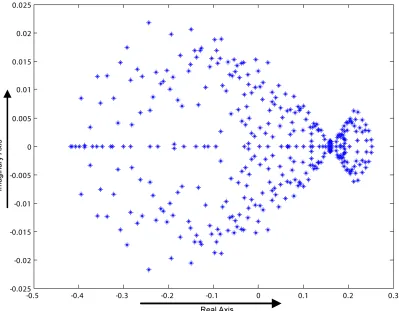
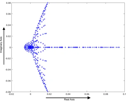
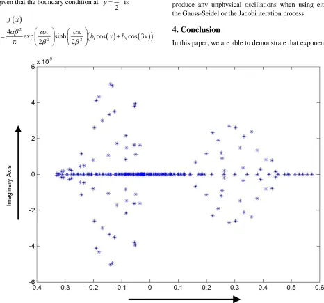
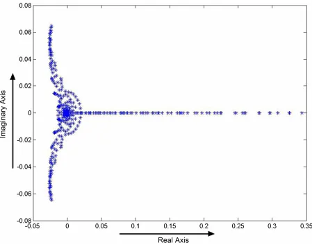
are applying the same idea, discussed in the i With this new system of equations, we analyze the spectral radii of the Jacobi and the Gauss-Seidel iteration matrices to determine whether the respective iterative processes will converge for large R values. Figures 3 and
4 show the eigenspectra of the respective iteration matri-ces when R = 100, a large value.
Au v,
eRxf v,
We see that in both cases the spectral radii of the tion matrices are less than one. This means that the itera-tions will lead to convergence. Our computaitera-tions show that this is indeed the case. Also, we do not get any un-wanted oscillations.
where
2 2
e Rx u u
Au
x x y
[image:3.595.101.500.406.717.2] and v H . H is the space of admissible test functions. Now, applying a Galerkin method we get
Figure 4. Eigenspectrum of the Gauss-Seidel iteration matrix with R = 100. In Table 1 we show the percentage error and the
num-ber of iterations for convergence (to the solution) for different values of R. In all the cases, the number of it-erations the Gauss-Seidel method took was less than half the number of iterations the Jacobi method took for con-vergence.
3. Convection Diffusion Transport Equation
In our previous model, the convection was only present in one spatial variable. In order to further investigate the effectiveness of this upwinding technique, we would like to explore a problem with convection on both spatial variables (x and y) and see what effects it has on the ei-genspectra of the Jacobi and the Gauss-Seidel iterative matrices.
For this purpose we analyze the following convection diffusion transport equation
(10) subject to the following boundary and initial conditions:
(11)
Table 1. Number of iterations and associated error for it-erative methods.
Jacobi method Gauss-Seidel method
R Percentage error No. of iterations Percentage error No. of iterations
10 0.009 523 0.009 251
50 0.052 62 0.052 24
100 0.087 70 0.087 19
150 0.106 91 0.106 24
Applying a Galerkin semi-discrete finite element method [5], in which we discretize only the spatial variables, we are left with the following system of ordinary differential equations:
2 2
0 , 0, 0
t xx yy x y
u u u u u t T
, , 0 , , ,
, , , , , , .
u x y f x y x y
u x y t g x y t x y
U U
B G b (12) where ij
j, i
j idx yd ,
B
2 2
,
d d ,
ij j i
j i j i i i
j j
a
x y
x x y y x y
G
,
,
i Wt i a W i
b .
[image:4.595.308.538.461.551.2]
, ,
W x y t
is a function that satisfies the boundary condition, and i
are the basic linear piecewise functions for i1,,N. In order to discretize in time, we will use the Crank- Nicolson method [6,7] and so, (12) becomes:
n 1 n n 1 n
U U U U
2
t
B G b
or
1
2 2
n n
t U t U t
B G B G b. (13)
Therefore, at each time step, we need to solve the lin-ear system (13). The stability of this method will depend on the amplification matrix [8]
1 2 2 t t
B G B G .
When and are small compared with 2 and
2
whe
not c we try
respectively, we will have convergence; n they large i.e., when convection is
onv o the orrect solution. In the to ve the system of linear equation Jacobi or the del iteration method, th
numerical solution for
however, domin
latter case, if
e spectral are erge t sol ( c Gauss-Sei the ant), the numerical solution will have oscillations and it will
s with the
[image:5.595.309.537.115.429.2] [image:5.595.62.284.547.709.2]radii of the iteration matrices will be greater than one.
Figure 5 shows 11, and one can clearly see the oscillations that result from Ja obi itera
a ltern directio plicit m with exp ntial u indi that pap he idea o ying exp ntial up din each spatial variable com s naturally
the syst variable at a time. So, it is he idea cussed in introduct will lead to good results.
c tions.
In [8] the authors address this problem by proposing
n a ating n im ethod one
pw ng. In er t f appl one
win
one is solving
g to e , since
em one
intuitive that t dis the ion
Figure 5. Numerical solution of (10)-(11) using 1000 itera-tions with α = 11 and γ = 11.
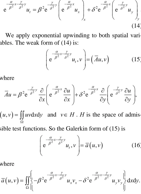
In this paper, to avoid the oscillations presented in the computed solution, we will rewrite Equation (10) as:
2 2 2 2 2 2 2 2
e e e e e
x y y x x y
t x y
y x
(14) We apply exponential upwinding to both spatial
vari-he weak form of (14) is:
u u u
. ables. T
2 2 e , x y tu v Au v
, w (15) here 2 22 2e e 2 u ,
2e e
x x
y u y
Au
x x y y
u v,
uv x yd d and v H
. H is the space of admis- sible test functions. So the Galerkin form of (15) is
2 2
e , ,
x y
t
u v a u v
(16) where
2 2 2 2 2 2, e e d .
x y x y
x x
a u v u v u v
Let d y y x y
, ,
U x y t be the Galerkin approximation for u(x, y,
t). Since we have an inhomogeneous Dirichlet boundary condition, we choose
1 , , , , , N i i iU x y t W x y t U t x y
(17)where i’s are the piecewise bilinear basis functions for 1, ,
i N, and i
x, ry condition and we wv y . satisfies the
ry condition to include it in our Galerkin approximation. So we have
where
, ,
W x y t
ill interpolate the bounda bounda
, 1 , 1
1
, , ,
N
i N i N i
W x y t U x y
, 1 , ,
i N i j k
U g x y t and i N, 1
on the bound
are the piece-ary. Now our Galerkin approximation takes the form
Substituting (17) into (16) we get the following system of ordinary differential equations in terms of t
wise bilinear basic functions
, 1 , 1
1 1
, , , ,
N N
i i i N i N
i i
U x y t U t x y U x y
.
d N
1 , , , , d0 for 1, ,
i j i j j i t i i
j
U t U a W a W
an
where are the solutions to the system
,N d the initial condition becomes
0 for 1, ,Uj cj j N
, 1, , j
c j N
1
, , for 1,
N
j i j i
j
c f i
.Written in matrix form we obtain
U U
B G b
where
,
,
,
and
,
,
ij j i ij a j i i Wt i a W i
B G b .
Applying the Crank-Nicolson method to discretize with respect to time, we have the new system of equatio given by
ns
1
2 n n U U t 1 n n
U U
B G or b
1
2 2
n n
t t
U U tb. (18)
B G B G
n be shown that this method is unconditionally stable [8].
In order to determine whether the iterative processe could produce a converging solution for (18), we analyze
ain, such that It ca
s
the spectral radii of the Jacobi and the Gauss-Seidel it-eration matrices.
For the numerical computations, we consider our equa- tion on a specific dom
2 2
, , , 0 t T
2 2
t xx yy x y
u u u u u x y
(19) with the following boundary conditions:
, 0,
u y y
2 2 2
, 0,
2 2 2
u x x
where , ,
2 2 2
u x f x x
0
2 2
f f
. For every computation ta
we ke 1, 1. We will take the steady state solution to be our initial condition and we will interpolate the boundary condition so that we have
where
, 1 , 1
1
, , ,
N
i N i N i
W x y t U x y
, 1
i N i
U f x and i N, 1
ns on the boundary
are the piecewise
bilinear basic functio y 2 fo r
2 x 2
r Gale pproximation takes
e, we have the
. So ou rkin a
the form
, 1 , 1
1 1
, , , ,
N N
i i i N N
i i
U x y t U t x y U x y
i .Henc linear system
1
2 2
n n
t t
U U t
B G B G
w
b
here Bij
j, i
,Gij a
j, i
and
, 1 , 1 1
, N
i
j j N j N i
U a
.
Using separation of variables [8], it is easy to show that the time dependent solution will tend to a stead
b
y state solution of the form:
2 2 2 1 2 1 2 1 1 ,u x y exp 2 2 2
exp 2 cos 2 1 d
cos 2 1 sinh 2
sinh
n
n
n
x y
f s s n s s
n x a y
a
(20)where
2 2 2 2 2 4 2
4 2 n
n
a
.
If f x
cos
x with 0, then (20) reduces to
2 2 2 21 2 1
4
sinh exp 2 2 2
2
cos 2 1 sinh 2
n n
x y
n x a y
(21) where 2 1 2 1 sinh n n b a
, u x y
2 4 2
2 2
2 4 2 4
4 1
4 1 4 1
n n b n n .
Notice that when 0 we ar
we get a steady state equa-tion similar to (5), so e interested in the case 0. For our numerical computations we will choose f x
such that the lution consists
two terms
steady state so of only the
,u x y
22 2
1
1
3
4
sinh exp
2
2 2 2
sinh
cos 3 sinh
2 sinh
x y
b
a
x a y
a
at the boundary condition at
2
1
cos sinh
2
x a y
3
3 b
given th
2
y is
2
1 3
2 2
4
exp sinh cos cos 3 .
2 2 b x b x
f x
We will take 1 5
t
, and 20
h for all our com - tions.
Figures 6 and 7 show the eigenspectra of the Jacobi and the Gauss-Seidel iteration matrices respectively when
10
puta
. We can clearly see that the spectral radii are less than one and so, we are sure to have convergence.
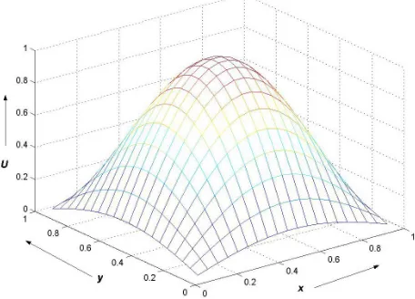
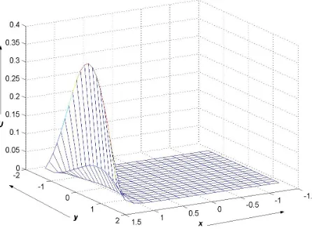
The graphs in Figure 8 show the steady state solutions when α= 10, γ = 1, and α= 1, γ = 10 respectively. Fig-ures 9 and 10 show the errors in the computed solutions when using the Gauss-Seidel iteration method with α = 10, γ = 1, and α= 1, γ = 10 respectively. The computed solutions with the Jacobi method are exactly the same the only difference is that the Gauss-Seidel method con-verges a lot faster. Also, the computed solutions do not produce any unphysical oscillations when using either the Gauss-Seidel or the Jacobi iteration process.
4. Conclusion
[image:7.595.60.526.274.709.2]In this paper, we are able to demonstrate that exponential ;
Figure 7. Eigenspectrum of the Gauss-Seidel iteration matrix for α = 10 and γ = 10.
(a) (b)
Figure 8. Analytical steady state solutions with (a) α = 10, β = 1, γ = 1, δ = 1 and (b) α = 1, β = 1, γ = 10, δ = 1.
upwinding is an extremely useful technique in convection diffusion computations. Even, if convection is dominant, employing exponential upwinding helps one to compute the solution without any difficulty. In particular, we have shown that one could easily use either the Jacobi or the
[image:8.595.65.537.446.645.2]Figure 9. Error in the computed solution when using Gauss- Seidel method with α = 10, β = 1, γ = 1, δ = 1.
Figure 10. Error in the computed solution when using Gauss- Seidel method with α = 1, β = 1, γ = 10, δ = 1.
corresponding iteration matrices are always found to be less than one. Thus, satisfying the condition for conver-gence of the chosen iteration process.
REFERENCES
[1] D. F. Griffiths and A. R. Mitchell, “On Generating Up- wind Finite Element Methods,” Finite ElementMethods forConvectionDominatedFlows, Vol. 34, 1979, pp. 91- 104.
[2] G. H. Golub and C. F. Van Loan, “Matrix Computations,” The Johns Hopkins University Press, Baltimore, 1990. [3] R. S. Varga, “Matrix Iterative Analysis,” Prentice-Hall,
Upper Saddle River, 1962.
[4] V. S. Manoranjan and R. Drake, “A Spectrum Enveloping Technique for Convection-Diffusion Computations,” IMA
Journal of Numerical Analysis, Vol. 13, No. 3, 1993, pp. 431-443. doi:10.1093/imanum/13.3.431
[5] R. Wait and A. R. Mitchell, “Finite Element Analysis and Applications,” John Wiley and Sons, New York, 1985. [6] A. R. Mitchell, “Computational Methods in Partial Dif-
ferential Equations,” John Wiley and Sons, London, 1969. [7] K. W. Morton and D. F. Mayers, “Numerical Solution of
Partial Differential Equations,” Cambridge University Press, Cambridge, 2001.
[8] V. S. Manoranjan and M. O. Gomez, “Alternating Direc- tion Implicit Method with Exponential Upwinding,” Com-