To what extent are financial crises comparable and thus predictable?

Munich Personal RePEc Archive

To what extent are financial crises

comparable and thus predictable?

Diamondopoulos, John

School of Management/Economics, Birkbeck College - University of

London, Department of Accounting, Finance and Economics

-European Business School London

16 October 2012

Online at

https://mpra.ub.uni-muenchen.de/45668/

1

To What Extent are Financial Crises Comparable and thus

Predictable?

John Diamondopoulos

This paper critically examines the quantitative approach to financial crises from two perspectives. First, the assumption of comparability of financial crises is analyzed. The key question here is: how

comparable are crises? Second, if financial crises are comparable to a certain extent, then we should be able to make predictions. Thus, the second key question is: how predictable are crises? The results have implications for the development of a theory of financial crises and government policies on crisis

management.

Key words: Financial crises, Crisis, Crisis Models, Crisis Management

JEL classifications: G01, G17, G18, H12

Introduction and Overview of Crises Explanation Frameworks

This paper is split into two sections. Part I is concerned with addressing the comparability of crises while Part II focuses on the question of crisis predictability. Before beginning our discussion, a brief overview of crises explanation frameworks is provided below.

Many attempts to explain and predict financial crisis have been made in the literature. Warneryd (2001:35) provides a rough categorization as follows:

1. Examination of general economic trends, business cycles, etc. 2. Search for long-term patterns in stock-price data.

3. Search for short-term patterns in stock-price data.

4. Assumptions about psychological changes, having to do either with learning (feedback) or with the diffusion and use of information.

5. Mass phenomena and social influences such as herd behaviour.

The first three reasons focus on indicators preceding turning points in an attempt to predict and/or point out warning signs before a crash. These explanations focus on the emergence of new information and are based on efficient market hypothesis and rational expectations theory assumptions.

However, as Warneryd (2001:31) notes when research takes behavioural data into account, theories become less abstract and more descriptive. Thus the theories become less able to explain and predict

a

School of Management/Economics, Birkbeck College – University of London, London, United Kingdom

2 bubbles in an all encompassing manner. Instead of a general theory, we start to view each bubble/crash as a specific case.

In short, crisis explanation frameworks can be reduced down to three categories from the five categories mentioned by Warneryd (2001:35):

1. Rational Expectations/Efficient Market Hypothesis (RE/EMH) explanations based on economic trends, business cycles and stock-price data (long and short term).

2. Psychological explanations which corresponds to the fourth category of Warneryd. 3. Sociological explanations which corresponds to the fifth category of Warneryd.

Finally, crises explanations can vary from reductionist attempts which try to cover everything in one general theory to non-reductionist specific case forms which take the view that each crisis is unique. RE/EMH explanations take the reductionist general theory approach, whereas the

Psychological/Sociological explanations tend towards the non-reductionist/specific case approach.

A similar line of reasoning is expressed in Allen and Gale (2007:24), who state that one of the main

themes in their book is that there isn’t one theory (‘The’ theory of crises) that can explain everything.

The reason is that crises are complex phenomena and thus a crisis may contain a combination of theories implying that theories of crises are not mutually exclusive.

For example, Allen and Gale (2007:1) pose the question: why did the dramatic events occur in Asia in 1997? To some this crisis was different. Previous crises in Mexico and Brazil could be attributed to inconsistent government macroeconomic policies – too small of a tax base relative to government expenditures in order to maintain a fixed exchange rate. Was it institutional factors – bank based

financial systems, lack of transparency, poor corporate governance, corruption? These can be reasons but all these factors were also present during a time when these countries were doing well.

‘Others blamed guarantees to banks and firms by governments or implicit promises of ‘bail-outs’ by organizations such as the International Monetary Fund (IMF). Rather than inconsistent macroeconomic policies being the problem, bad microeconomic policies were the problem. Either way it was

governments and international organizations that were to blame.’ (Allen and Gale 2007:1) In addition,

Allan and Gale (2007:1) note that crises ‘…have not been restricted to emerging economies even in recent

times. The Scandinavian crises of the early 1990s are examples of this. Despite having sophisticated economies and institutions, Norway, Sweden and Finland all had severe crises. These were similar in

many ways to what happened in the Asian crisis of 1997.’ Krugman (2008:5) states that the Asian crisis

of 1997 was a sort of rehearsal act for the current credit crisis.

The comparison of different crises is constantly made in academic studies and in the media as exemplified above. However, the assumption of the comparability of crises is not always made explicit or critically examined.

3 RE/EMH theories) are questionable. The implications are that a theory of crises based on RE/EMH explanations using a large N research design might not be achievable.

Large-N studies require the assumption that crises are comparable because the purpose of these studies is to be able to predict crises. Thus, of primary importance to RE/EMH models is the following question – How predictable are crises?

A large factor in the success or failure of large-N studies thus derives from the extent of comparability among crises or as stated earlier as a question – How comparable are crises?

In short, the question of ‘How predictable are crises?’ is intimately tied to the question of ‘How comparable are crises?’ In order words, the extent of comparability will determine the extent of

predictability.

Part I. The Comparability of Financial Crises

This is by no means a comprehensive look at the literature. Rather the focus, besides addressing the question of whether crises are comparable, is on highlighting the often ignored role of context in quantitative studies. Two seminal studies – Reinhart and Rogoff (2009) and Bordo et al (2001) are discussed in detail.

Historical studies which compare various crises over long periods of fifty to seventy plus years have been conducted. However, the main problem with this type of analysis is the assumption of ‘all things being equal.’ Allen and Gale (2007:2) note that the period from 1945 to 1971 was exceptional since only one banking crisis occurred – Brazil in 1962. The reasons behind the lack of banking crisis during this period were the result of extensive regulation. In the US, the Federal Reserve System was put in place in the 1930s along with extensive financial regulation. Other countries even had more regulation because the allocation of funds was through state-owned banks or heavily regulated ones. But the elimination of banking crisis had a cost – inefficient allocation of funds by the financial system. Allen and Gale

(2007:2) citing Bordo et al. (2001) state that deregulation made the period after 1971 more like the period before 1914.

The idea that there are some periods more or less prone to crises is a common theme in the literature. Bordo et al (2001) pose this same question in their study –‘Is the Crisis Problem Growing More Severe?’ Bordo et al (2001:53-54) state that this question has not been studied expect for a few studies which compare the ‘…1990s with the preceding decades (e.g., International Monetary Fund, 1998; Caprio and

Klingebiel, 1999) …A comparison of the 1980s with the 1990s is hardly an adequate basis for generalization, of course.’ For Bordo et al (2001), the time period needs to be extended back much further in order to gain historical perspective. In their study, the time period covered is 120 years. The reason is that two main views exist regarding the frequency and severity of crises. One view points to the dangers of financial liberalization coupled with the inefficient allocation of resources by the financial markets. The other view places the problem squarely on governments running inconsistent monetary and fiscal policies based on exchange rate and financial stability combined with the weakened market

4 What is revealing about the Bordo et al (2001) study is not the time period, but their implicit recognition that comparisons extending back 120 years in history, from 1880 to 1997, are fraught with potential context compatibility problems. The solution they implement is to divide this time period into four distinct periods - 1880-1913(gold standard era), 1919-1939 (interwar years), 1945-1971 (Bretton Woods period) and 1973-1997 (flexible exchange rate period). The period from 1973-1997 consists of two data sets containing 21 countries and 56 countries. The reason for two data sets in this period is to keep the comparisons consistent with earlier time periods (21 country data set) and with more recent time periods (the 56 country data set). Bordo et al (2001:54) base the comparison on four dimensions:

1. The four distinct time periods (as discussed above).

2. The average frequency, depth and duration of crises in each time period.

3. The severity of the crises in each time period (compare output lost to recessions with no crisis).

4. Determine if the patterns observed are the result of international economic policies (flexible FX rates and openness of capital account) or the management of domestic financial system. It should be noted that this corresponded to the two leading explanations of the Asian crisis at the time.

First, the four distinct time periods as defined by Bordo et al (2001) are essentially based on the international monetary regimes during the respective time periods. The assumption is that the external financial regime prevailing during those four distinct time periods is homogeneous and other important dimensions are either ignored or considered not relevant. For example, during the 1973 to 1997 time period, the use of financial derivatives became prevalent. However, the sophistication and

implementation of derivatives was not homogeneous throughout this time period. Mutual funds in the US until very recently were prohibited from employing derivatives. In addition, the rapid growth of hedge funds in recent years increased the use of derivatives in actual trading strategies. Thus, the impact and use of derivatives varied throughout this time period. And this has important implications for market volatility and stability. Jacobs (1999) attributes the market crash of 1987 in the US to portfolio insurance, a derivatives product made very popular by two University of California, Berkley finance professors – Leland and Rubinstein. Derivatives had just come on their own at about the mid-80s, having appeared in the 70s it took time for the market to accept their use as the products grew more sophisticated.

Second, Bordo et al (2001) are correct in criticizing prior studies that only covered a time period of a few decades since not enough crises would have occurred in this time frame to make generalizations, or more importantly statistically valid generalizations. And this is the essence of quantitative large N studies. That is why their sample size includes 21 countries and goes back 120 years.

Third, the crises types as defined in this study are only two – currency crises and banking crises – or a combination of these two types – twin crises. The classification of crises into different types has important implications for the comparability of crises. In fact, Bordo et al (2001:59) in a footnote state,

‘The Goodhart-Delargy conclusion is based on an analysis of only six episodes. Moreover, we categorize some of their currency crises as twin crises (Italy, 1894 and 1908, Argentina, 1890) or banking crises

5 As discussed above, it can be seen that additional difficulties with historic comparisons are the

measurement of the economy and crises type. For example, Allen and Gale (2007:5) note that ‘Economic historians often use production of pig iron as a proxy for GDP.’ This was used to measure the seriousness

of a crisis.

Calomiris in Durlauf and Bloom (2010:14) states, ‘There are two distinct phenomena associated with banking system distress: exogenous shocks that produce insolvency and depositor withdrawals during

‘panics’. These two contributors to distress often do not coincide.’ The example is given of how in the

Rural United States of the 1920s, many banks failed and how high losses to depositors did not coincide with systematic panics. In contrast, systematic panic was present during the 1907 crisis which originated in New York. The losses to depositors during the 1907 crisis were slightly higher than normal times.

Referencing a book by Bruner and Carr (2007), titled ‘Money Panic: Lessons from the Financial Crisis of

1907’, Calomiris in Durlauf and Bloom (2010:14) emphasizes that the main difference between these two cases lies in information commonality regarding the shocks produced by the loan losses. They state that,

‘In the 1920s, the shocks were loan losses in agricultural banks, geographically isolated and fairly transparent. …During 1907, the ultimate losses for New York banks were small, but the incidence was

unclear ex ante (loan losses reflected complex connections to securities market transactions, with uncertain consequences for some New York banks). This confusion hit the financial system at a time of

low liquidity, reflecting prior unrelated disturbances in the balance of payments.’

Thus, it can be seen that causes, market reactions and remedies even vary within a crises category. The result is that the information lost which occurs when context is taken out when conducting a large N study can be substantial. This has implications for the comparability and ultimately the predictability of crises.

Fourth, Bordo et al (2001) do not discuss the differences between the countries nor how these individual countries varied over time. This is normal when conducting large N studies. The assumption is that the differences will on average cancel out. But what if this is not the case?

For example, differences in the development of central banks in three countries (UK, US and Canada) might have affected the prevalence and propagation of crises in the early part of the 20th century.

It is important to take note of differences within countries when conducting historical analysis. For

example, Allen and Gale (2007:3) state, ‘There was no central bank in the US from 1836 until

1914…Kindleberger (1993) points out that many British economists ascribe the absence of crisis in the

UK to central banking experience gained by the Bank of England and their ability to skillfully manipulate

discount rates.’ In the US, Allen and Gale (2007:5) note that the 1907 banking panic started the debate on

the need of a central bank which was established in 1914. But the creation of the FED did not stop

banking panics since ‘it had a regional structure and decision making power was decentralized.’

6 In addition, to the points made previously, it should be mentioned that politics plays a major role during crises. It is worth noting that the importance of politics and policy is mentioned extensively in their comprehensive study on the history of financial crises –‘This Time is Different’– by Reinhart and Rogoff (2009) but not analyzed or taken into account during their extensive study. The addition of political and policy considerations make it more difficult to compare crises.

Another complication is the availability and comparability of data over long periods of time which Reinhart and Rogoff (2009) consistently mention as a major hurdle in their work.

A key theme throughout the book by Reinhart and Rogoff (2009) is the idea that market participants and

policy makers miss crises because of the belief that ‘this time is different’ which is also the title of the

book. Although not explicitly stated, the theme of ‘this time is different’ implies that sociological aspects play a key role in a crisis.

Although the book by Reinhart and Rogoff (2009) does not particularly focus on the political and sociological aspects of crises, these aspects will be mentioned under the various types of crises which were identified in the book. In addition, the availability and quality of data when mentioned will be noted.

Reinhart and Rogoff (2009:xxvii) criticise recent studies which only use a data set going back to 1980s on the grounds of most readily accessible. Reinhart and Rogoff (2009:xxvii –xxviii) state, ‘This approach would be fine except for the fact that financial crises have much longer cycles, and a data set that covers twenty-five years simply cannot give one an adequate perspective on the risks of alternative policies and investments. An event that was rare in that twenty-five year span may not be all that rare when placed in a longer historical context. After all, a researcher stands only a one-in-four chance of observing a

“hundred-year flood” in twenty-five years’ worth of data. To even begin to think about such events, one needs to compile data for several centuries.’

Discussing the available data going back centuries, Reinhart and Rogoff (2009: xxviii), mention variables such as: domestic and external debt, inflation, GDP, interest rates and the prices of commodities.

In addition, they note the extreme difficulty of obtaining domestic debt data. Interestingly, Reinhart and Rogoff (2009:xxxi) note, ‘That the history of domestic public debt …in emerging markets, in particular, has largely been ignored by contemporary scholars and policy makers (even by official data providers

such as the International Monetary Fund)…’

Reinhart and Rogoff (2009: xxxi) attempt to address the fact that prior studies have ignored domestic debt

by offering ‘…a first attempt to catalog episodes of overt default on and rescheduling of domestic public

debt across more than a century. (Because so much of history of domestic debt has largely been forgotten by scholars, not surprisingly, so too has its history of default). This phenomenon appears to be somewhat rarer than external default but is far too common to justify the extreme assumption that governments always honor the nominal face value of domestic debt, an assumption that dominates the economics

literature.’ It is acknowledged that default on domestic debt occurs under a higher hurdle. The reason

7 Reinhart and Rogoff (2009: xxxiii) further stress the importance of government debt and politics,

‘Although private debt certainly plays a key role in many crises, government debt is far more often the

unifying problem across a wide range of financial crises we examine. …the fact that basic data on

domestic debt are so opaque and difficult to obtain is proof that governments will go to great lengths to hide their books when things go wrong, just as financial institutions have done in the contemporary

financial crisis.’

In the next paragraph, Reinhart and Rogoff (2009: xxxiv) stress the paramount importance of sociological

factors, but don’t develop the idea further besides the following statement, ‘…the most expensive

investment advice ever given in the boom just before a financial crisis stems from the perception that

“this time is different”. …Financial professionals and, all too often, government leaders explain that we are doing better things better than before, we are smarter, and we have learned from past mistakes.

…Each time, society convinces itself that the current boom, unlike the many booms that preceded

catastrophic collapse in the past, is built on sound fundamentals, structural reforms, technological

innovation, and good policy.’

In short, the illusion is that better models by market participants and better policy by governments will prevent the next crisis. Thus, in any theory of crises, sociological and political factors must take center stage.

Before examining social and political factors in more detail, what defines crises is an important

consideration in addressing the question of whether or not crises are comparable. Reinhart and Rogoff

(2009:4) in discussing the definition of crises state, ‘…it may be possible, in principle, to have systematic

definitions of crises. But for a number of reasons, we prefer to focus on the simplest and most transparent delineation of crisis episodes, especially because doing otherwise would make it very difficult to make

broad comparisons across countries and time. …We begin by discussing crises that can readily be given

strict quantitative definitions, then turn to those for which we must rely on more qualitative and

judgemental analysis.’

Reinhart and Rogoff (2009:4-8) define crises in two major camps – crises defined by quantitative thresholds and crises defined by events. The quantitative threshold category of crises – inflation, currency crashes and currency debasement – use arbitrary thresholds to define a crisis. For example, the chosen thresholds adopted are: 20% for inflation crises, 25% for currency crises and 5% for a Type I currency debasement (metallic content of coins) and the term ‘much-depreciated’ for a Type II currency debasement (new currency replaces old).

On the threshold for inflation crises, Reinhart and Rogoff (2009:5-6) make the following comments, ‘A number of studies, including our own earlier work on classifying post-World War II exchange rate arrangements, use a twelve-month threshold of 40 percent or higher as the mark of a high-inflation episode. Of course, one can argue that the effects of inflation are pernicious at much lower levels of inflation, say 10 percent, but the costs of sustained moderate inflation are not well established either

theoretically or empirically. …Hyperinflations – inflation rates of 40 percent per month – are of modern vintage. For the pre-World War I period, however, even 40 percent per annum is too high an inflation threshold, because inflations rates were much lower then, especially before the advent of modern paper

8 Asset price bubbles in equity or real estate are particularly problematic from a data point of view since they are either not available or very difficult to attain in long run cross-country studies, except in the last couple of decades according to Reinhart and Rogoff (2009: 7-8).

Thus, equity and real estate bubbles are discussed under banking crises. Additionally, the reason for placing banking crises in the crisis category defined by events is lack of long-term time series data which impacts the quantitative dating for banking crisis in a similar way to inflation or currency crises,

according to Reinhart and Rogoff (2009:8). Indicators such as the relative price stock price of banks fail since many developing country banks, especially in the past, did not have banks that were publically traded. Another indicator, changes in bank deposits also fails since it applies more to bank panics in the 1800s.

As can be seen by these examples, defining and measuring a crisis for comparison purposes is difficult due to the unavailability of data or common data over time. In addition, the magnitude of the quantitative measure can change depending on the time period. All of these issues may result in a case of comparing

‘apples’ with ‘oranges.’ And this has important implications for the large N studies, especially in terms

of validity.

It is important to note that even in a quantitative study of crises; the definition of some crises relies heavily on qualitative judgement. Reinhart and Rogoff (2009:3-4) state that the boundaries they define of what is or what is not a crisis are close to the existing empirical literature. Some of the definitions rely more on qualitative judgement, whereas others can be given strict quantitative definitions.

What should be noted is that the Reinhart and Rogoff (2009) boundaries on crises are close to the empirical literature since Reinhart and Rogoff are major contributors to that literature. For example, if one looks at Appendix A.4 Historical Summaries of Banking Crises of Reinhart and Rogoff (2009), there are a few authors that are cited multiple times. The most commonly cited authors are Conant in the early 1900s, Caprio and Klingebiel, Reinhart and Rogoff, Bordo and Eichengreen, Kaminsky and Reinhart, Bordo et al., Bernanke and James, Jacome, and several authors focusing on regional crises. The empirical literature boundaries and thus definition of a banking crisis are heavily influenced by about ten authors and if we take into account that most of these authors write joint papers, this number drops down to around six main contributors. Thus, the definitions and boundaries of what constitutes a banking crisis are heavily influenced by approximately six main authors or author pairs. Appendix A.4 does not cover all the authors, but it is an extensive data set covering the period from 1800 to 2008 with the main academic sources listed under each banking crisis. Information is not provided regarding other types of crises, thus it is not know if this holds true for other types of crises. This would be an interesting area for future research.

9

Table1: Definition of Crises

Category 1: Crises Defined by Quantitative Thresholds

Crisis Type Definition Sub-Types and Additional Information

Inflation Post WWII – many studies use an inflation

rate of ≥ 40%

Pre WWII – a lower inflation rate threshold of

≥ 20% , although rates of 15-25% can be used

No sub-types are listed, but the main dividing line is pre and post WWII.

Currency Crashes Post WWII - use the Frankel & Rose

approach of large currency depreciations of 25%

Pre WWII – 15%

No sub-types are listed, but the main dividing line is pre and post WWII.

Currency Debasement Precursor to modern inflation and FX crises in

era of metallic coins and defined as reduction of metallic content by ≥ 5%

Modern –currency ‘reforms’ or conversions where new currency replaces the old

Currency ‘reforms’ or conversions are part of

hyperinflation episodes and occur multiple times. Examples include Brazil (1986-1994) which had about 4 currency conversions.

Crises defined by Quantitative Thresholds but not listed as a separate category.

Asset Price Bubbles

Equity

Real Estate

Corporate Defaults

None provided, but on page 8 it is noted that asset price bubbles are common before the onset of a banking crisis.

None provided for corporate defaults.

Housing price data is very difficult to obtain while equity price data is only available for past couple of decades on a cross-country basis.

Housing and corporate defaults are ‘crisis types’, but due to data issues, these two types are captured in within the bank crisis data. These two types of crises lead to bank defaults (justified on page 251).

Category 2: Crises Defined by Events

Crisis Type Definition Sub-Types

Banking Crises Bank runs or large-scale government

assistance to banks.

Type I: Systematic (Severe)

Type II: Financial Distress (Milder)

Difficult to date the start and end of the banking crises.

External Debt Crises Failure of government to meet principle or

interest payment.

Clear start and end date, but sometimes final resolution never takes place which makes the end date indeterminate.

Domestic Debt Crises Same as external debt crisis, but on domestic side. Also can include freezing bank deposits, forced conversions of deposits from foreign currency (dollars) to local currency.

Historically, difficult to date these crises and like bank crises difficult to date the end.

Source: Adapted by the author from Reinhart and Rogoff (2009) Tables 1.1 and 1.2

10 First, three unlisted quantitative threshold type crises – equity, real estate and corporate default – are grouped under banking crises, which are defined by events. Reinhart and Rogoff (2009: 249-251) cover all three types in their composite BCDI index, which is designed to measure crisis severity. The six crisis categories are reduced to five with currency debasement being merged with currency crises. Although bundled up with bank crises initially, in the composite BCDI index equity crises are accounted for separately while real estate and corporate are still bundled up with banking crises. Reinhart and Rogoff (2009: 249-251) state,

‘Where feasible, we also add to our five-crisis composite a “Kindleberger-type” stock market crash, which we show separately. In this case, the index runs from zero to six. …the Black Monday crash of October 1987… is not associated with a crisis of any

other stripe. …there are two other important dimensions of defaults that our crisis index does not capture directly. First, there are

defaults on household debts …for instance, have been at center stage in the unfolding subprime saga …However, such episodes

are most likely captured by our indicator on banking crises. More problematic is the incidence of corporate defaults, which are in

their own right another “variety ofcrises.” This omission is less of an issue in countries where corporations are bank-dependent.

… For countries with more developed capital markets, it may be worthwhile to consider widespread corporate default as yet

another variety of crisis. …the United States began to experience a sharp run-up in the incidence of corporate default during the

Great Depression well before the government defaulted …it is worth noting that corporate defaults and banking crises are indeed correlated, so our index may partially capture this phenomenon indirectly.’

What is important to note is that equity crises are included in the index, but real estate and corporate defaults are not. It is assumed that both real estate and corporate default type crises may be captured in the banking crisis category.

Second, the Black Monday crash of October 1987 is not considered in the equity crisis category. What category is it in? Reinhart and Rogoff (2009) do not answer this question. The Black Monday crash of October 1987 is an important crisis, especially as it relates to the subsequent development of derivative prices which has impacted the market ever since. Fear of such a crash occurring again can be seen in option prices with volatility smiles. In other words, out of the money puts have a higher volatility component imbedded in the pricing. Thus, the market has still not forgotten this crisis.

In addition, there are several problems associated with what Reinhart and Rogoff (2009) term global crises. For example, in which crisis category do global financial crises fit? It is evident from the definition given to global crises by Reinhart and Rogoff (2009) that these crises are on a different scale, thus do global crises really fit under any of the Reinhart and Rogoff categories?

Only six episodes of global financial crises are highlighted when using the definition of global financial crises as proposed by Reinhart and Rogoff (2009: 261 in Box 16.1). Highlighted global financial crises include: The Crisis of 1825-1826, The Panic of 1907, The Great Depression 1929-1938, Debt Crisis of the 1980s, The Asian Crisis of 1997-1998, The Global Contraction of 2008. Reinhart and Rogoff (2009:

270) in discussing global crises note, ‘We have hundreds of crises in our sample, but very few global

ones, …and some of the earlier global crises were associated with wars, which complicates comparisons even further.’

Reflecting on global crises, Reinhart and Rogoff (2009: 269) state, ‘…global financial crises can be so

11 In short, global financial crises pose two main problems for comparability. First, comparative country indicators tend to move in tandem and second, there are too few global financial crises to test which makes empirical tests difficult.

Finally, the crises categorization of Reinhart and Rogoff (2009) and Bordo et al (2001) are different which would make comparisons between two important long-term quantitative studies on crises difficult. Even the severity indicators used are different.

What is clear from both of these seminal studies – Reinhart and Rogoff (2009) and Bordo et al (2001) – is that it is very difficult to compare crises over the long term due to data issues, measurement issues, contextual factors (institutional, social and political) and crisis definitions. In addition, the occurrence of crises span many years, thus as Reinhart and Rogoff (2009) and Bordo et al (2001) state, data sets of 25 years or longer are needed to place a particular crisis in the proper historical perspective.

In short, the danger with large-N studies over the long term is that the context has already been removed while the danger with large-N studies over the short term is on finding enough comparable cases.

PART II

–

The Predictability of Financial Crises

Reinhart and Rogoff (2009: x) in the Preamble section, state, ‘This book summarizes the long history of

financial crises in their many guises across many countries. …this chapter will attempt to sketch an economic framework to help the reader understand why financial crises tend to be both unpredictable and

damaging. …economic theory proposes plausible reasons that financial markets, particularly ones reliant

on leverage …can be quite fragile and subject to crises of confidence. Unfortunately, theory gives little guidance on the exact timing or duration of these crises…’

The previous statement by Reinhart and Rogoff (2009) implies that predicting crises is very difficult. If crises were comparable to a certain extent, then it would be logical to assume that they can be predicted. Next, we will look at some of the empirical evidence.

The modelling of crises generally falls into two categories –probit/logit models or the ‘signals’ approach. Mariano et al (1999:1-2) states, ‘The relatively more popular approach is to use probit/logit models (As illustrated by Eichengreen and Rose (1998) for currency crises and Demirguc-Kunt and Detragiache

(1998) for prediction of banking crises. … Alternatively, the methodology adopted by Kaminsky and Reinhart (1996) and Kaminsky, Lizondo and Reinhart (1998) is known as the ‘signals’ approach which

essentially optimizes the signal to noise for the various potential indicators of crisis.’

The Kaminsky, Lizondo and Reinhart (1998) study is representative of the ‘signals’ approach. The

authors examine leading indicators of currency crises and note that forecasting and timing currency crises is likely to remain an elusive goal. In addition, this study is also a meta-study of prior papers using probit/logit models.

In their comparison of 28 empirical studies on currency crises, Kaminsky et al (1998:7) emphasize that one of the difficult issues they dealt with when comparing these studies was the variability among the

studies in how they defined a crisis. ‘Most of the studies focused exclusively on devaluation episodes.

12 frequent devaluations that may not fit the mold of a full-blown currency crisis. A few studies adopt a broader definition of crises. They include, in addition to devaluations, episodes of unsuccessful speculative attacks; that is, attacks that were averted without a devaluation, but at the cost of a large

increase in domestic interest rates and/or a sizable loss of international reserves.’

How one defines a crisis has implications for comparability and subsequently predictability. If crises were easily comparable, then one would expect the definition of a crisis to be pretty consistent among various studies. And as was previously mentioned, if crises were pretty comparable, predicting crises would be easier. Consequently, most studies would agree on similar leading indicators. Instead, Kaminsky et al (1998:23) conclude that a broad set of indicators is advised for an effective warning system for currency

crises. ‘…and these crises are usually proceeded by symptoms that arise in a number of areas.’

The set of indicators totals 105 from the 28 empirical studies in Kaminsky et al (1998:9) and are broken down into six broad categories plus contagion by the authors. The following tables 2 and 3 are adapted from Table A2 and the broad category summary of indicators in Kaminsky et al (1998: Table A2 on pages 36-37 and broad category summary on pages 9-10, respectively):

Table 2: Total Number of Crisis Indicators from 28 Empirical Studies

Main Category

External Financial Liberalization

Real Sector Fiscal Institutional Structural

Political Contagion

Sub-Category Capital Account

Debt Profile

Current Account

International

Financial Liberalization

Other Financial

Real Sector Fiscal Institutional

Structural

Political Contagion

Total Indicators 105

49 21 9 6 10 9 1

Source: Adapted from Table A2, Kaminsky et al (1998:36-37)

It should be noted that although 105 indicators are listed, overlaps do exist. As discussed by Kaminsky et

al (1998:9), ‘…that many of the indicators listed in Table A2 are transformations of the same variable. For instance, several variables are expressed alternatively in levels or in rates of change; sometimes on their own and other times relative to some standard (such as the same variable in a trading partner). …The use of scale factors also varies across studies. For example, alternative scale factors used for international

reserves include GDP, base money, M1, M2, and the level of imports.’

13

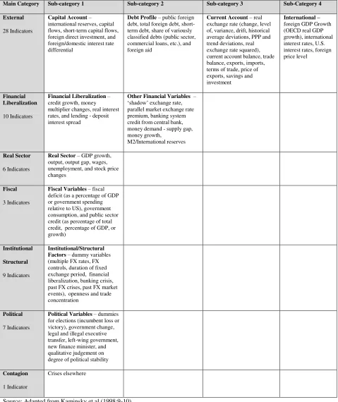
Table 3: Crisis Indicator Classifications – Broad and with consolidated Sub-categories

Main Category Sub-category 1 Sub-category 2 Sub-category 3 Sub-Category 4 External

28 Indicators

Capital Account–

international reserves, capital flows, short-term capital flows, foreign direct investment, and foreign/domestic interest rate differential

Debt Profile– public foreign debt, total foreign debt, short-term debt, share of variously classified debts (public sector, commercial loans, etc.), and foreign aid

Current Account– real exchange rate (change, level of, variance, drift, historical average deviations, PPP and trend deviations, real exchange rate squared), current account balance, trade balance, exports, imports, terms of trade, price of exports, savings and investment

International –

foreign GDP Growth (OECD real GDP growth), international interest rates, U.S. interest rates, foreign price level

Financial Liberalization

10 Indicators

Financial Liberalization–

credit growth, money multiplier changes, real interest rates, and lending - deposit interest spread

Other Financial Variables –

‘shadow’ exchange rate,

parallel market exchange rate premium, banking system credit from central bank, money demand - supply gap, money growth,

M2/International reserves

Real Sector

6 Indicators

Real Sector– GDP growth, output, output gap, wages, unemployment, and stock price changes

Fiscal

3 Indicators

Fiscal Variables– fiscal deficit (as a percentage of GDP or government spending relative to US), government consumption, and public sector credit (as percentage of total credit, percentage of GDP, or growth)

Institutional Structural

9 Indicators

Institutional/Structural Factors – dummy variables (multiple FX rates, FX controls, duration of fixed exchange period, financial liberalization, banking crisis, past FX crises, past FX market events), openness and trade concentration

Political

7 Indicators

Political Variables– dummies for elections (incumbent loss or victory), government change, legal and illegal executive transfer, left-wing government, new finance minister, and qualitative judgement on degree of political stability

Contagion

1 Indicator

Crises elsewhere

14 Kaminsky et al (1998:7-8) grouped the selected 28 empirical studies into four categories. The first group of four papers were mainly qualitative in nature and did not conduct any formal tests on the crisis

indicators identified. The second group of five papers looked at the periods before and after the crisis, but had inconsistencies in terms of narrowing down potential variables. The third group of fifteen papers estimated probabilities of devaluation in future periods based on explicit theoretical models. The fourth group of two papers used the signals approach.

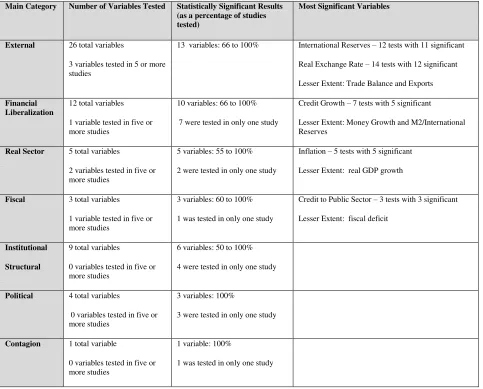
In order to identify the most useful indicators for crisis prediction, Kaminsky et al (1998:10-11) narrowed down the list of 28 empirical studies to 17. Essentially they excluded most the papers from the first two categories mentioned above due to lack of formal tests. This meant that only those indicators that were featured in the 17 studies were taken into account. Table 4 below provides a summary of the total variables under each category that were tested and found to be statistically significant and a listing of the key variables:

Table 4: Statistical Significance Summary of Main Categories and Specific Variables

Main Category Number of Variables Tested Statistically Significant Results (as a percentage of studies tested)

Most Significant Variables

External 26 total variables

3 variables tested in 5 or more studies

13 variables: 66 to 100% International Reserves – 12 tests with 11 significant

Real Exchange Rate – 14 tests with 12 significant

Lesser Extent: Trade Balance and Exports

Financial Liberalization

12 total variables

1 variable tested in five or more studies

10 variables: 66 to 100%

7 were tested in only one study

Credit Growth – 7 tests with 5 significant

Lesser Extent: Money Growth and M2/International Reserves

Real Sector 5 total variables

2 variables tested in five or more studies

5 variables: 55 to 100%

2 were tested in only one study

Inflation – 5 tests with 5 significant

Lesser Extent: real GDP growth

Fiscal 3 total variables 1 variable tested in five or more studies

3 variables: 60 to 100%

1 was tested in only one study

Credit to Public Sector – 3 tests with 3 significant

Lesser Extent: fiscal deficit

Institutional Structural

9 total variables

0 variables tested in five or more studies

6 variables: 50 to 100%

4 were tested in only one study

Political 4 total variables

0 variables tested in five or more studies

3 variables: 100%

3 were tested in only one study

Contagion 1 total variable

0 variables tested in five or more studies

1 variable: 100%

1 was tested in only one study

15 Kaminsky et al (1998:12) note several problems with drawing conclusions from the comparison of the 28 empirical studies (later 17 studies were actually used). First, the comparisons were not conclusive in terms of which indicators were the most useful in predicting currency crises. The reason for this non-conclusiveness is a result of the large number of indicators among the studies and other factors – different variable measurements, different time periods of the data, estimation techniques. Additionally, some variables are significant in univariate tests but not in multivariate tests. However, Kaminsky et al (1998:12-13) draw the following conclusions:

1. A broad variety of indicators need to be included in an effective early warning system (EWS). The reason is that currency crises can develop from multiple economic and political problems.

2. Several indicators had enough support to serve as useful currency crisis indicators. Please refer to the Table 5 above, Most Significant Variables column.

3. The other indicators are inconclusive because only one or two studies covered reviewed them.

‘…several foreign, political, institutional, and financial variables …have some predictive power in anticipating currency crises. Banking sector problems stand out in this regard…’ In addition, the contagion variable stands out.

4. ‘…the variables associated with the external debt profile did not fare well. Also, contrary to expectations, the current account balance did not receive much support as a useful indicator of

crises.’ The current account balance effect may be included in the real exchange variable (which proved statistically significant when the current account balance did not in the same studies).

5. ‘…market variables, such as exchange rate expectations … and interest rate differentials …did not do well in predicting currency crises, whether these were preceded or followed by

deteriorating economic fundamentals or not. This call into question the assumption embedded in most of the theoretical models, whether these are the first or second generation variety – namely,

that rational agents know the ‘true’ model and embed that into their expectations.’

An interpretation of the comments by Kaminsky et al (1998) would conclude that performing a meta-study on currency crisis empirical literature is difficult. This might be because crises themselves are difficult to compare. This is further supported by the fact that Kaminsky et al (1998) strongly conclude that a broad variety of indicators is needed due to the multiple economic and political sources of currency crises. Some of the variables (external debt profile, current account balance, exchange rate expectations and interest rate differentials) which were predicted theoretically surprisingly were not relevant. Finally, two important points as follows:

1. The assumption of ‘rational agents’ is questioned.

2. The potential importance of political and institutional factors is mentioned.

The second point on political and institutional factors is further emphasized by Kaminsky et al (1998:24) in the conclusions as follows:

16

a political and institutional nature, that may be relevant for a particular country at a particular moment in time, and that are not incorporated in the warning system. A comprehensive assessment of the situation would necessarily need to take those issues into

account. Only then would it be possible to have a coherent interpretation of events and a firm base for policy decisions.’

In short, the Kaminsky et al (1998) highlight the difficulties of crisis prediction. Next, a study by Poltenen

(2006) is discussed in that it compares the Kaminsky et al (1998) ‘signal approach’ model to the standard

probit model and several other models.

Poltenen (2006:5-8) reaches the conclusion in his paper titled, ‘Are Emerging Market Currency Crises

Predictable? A Test’ that ‘… the ability of the models to predict currency crises out-of-sample was found

to be weak … certain factors were found to be related to the emerging market crises. These factors are

the contagion effect, the prevailing de facto exchange rate regime, the current account and government budget deficits, as well as real GDP growth. Furthermore, it appears that economic fundamentals were able to statistically better explain the onset of currency crises in the subsample of the 1980s than in the subsample of the 1990s, where other variables, such as the contagion effect, were statistically significant. This confirms earlier findings in the literature that the contagion effect versus economic fundamentals might have played a greater role in the onset of the currency crises in the 1990s, in contrast to the crises of

the 1980s. …Finally, the results reinforced the view that developing as stable model capable of predicting or even explaining currency crises can be a challenging task.’ What is especially relevant regarding the comments made by Poltenen (2006) is that indicators, such as contagion, can change dramatically in terms of importance over time.

Poltenen tested probit models and a multi-layer perception artificial network (ANN) model using

‘commonly used’ crisis indicators. Poltenen (2006:18-20) evaluated these models using cross-tabulations of correct classifications, different goodness-of-fit measures such as: Brier’s Quadratic Probability Score (QPS), the Receiver Operating Characteristic (ROC) and Cramer’s Gamma. ‘Finally in-sample and out-of-sample predicted probabilities for the countries were plotted to illustrate the ability of the models to

predict crises. … However, as in the case of in-sample estimations, the information set is larger than the economic agents had at each time, and therefore, the true predictive power of the models was evaluated using the out-of-sample forecasts. …the in-sample forecasts can be thought of only as a measure of goodness-of-fit of the models.’

The results are then discussed by Poltenen (2006:20-21), ‘…the out of sample data contains 56 crises periods of which the models were able to predict a maximum of 4 periods using the lowest level of 0.10. In addition, the other goodness-of-fit measures also point out that the out-of-sample forecasts are not

particularly strong.’

In his comparison with selected earlier papers, Poltenen (2006:21) makes some important points. First,

‘the comparison of results between different papers is not straightforward as the estimation samples, countries included, the threshold values as well as the crisis window differ. However, it has become a

standard to benchmark the obtained results to the ‘signal approach’ developed by Kaminsky et al. (1998),

as well as the standard probit model.’ Second, only a few of the earlier studies have reported both in -sample and out-of--sample results making comparisons difficult. Third, Poltenen (2006:34) shows that the in-sample results were similar to prior studies; however the out-of-sample results were much weaker than

17 models were required to predict crises truly out-of –sample without using information that was potentially not available to economic agents at the time. In addition, the models were being classified as being able to predict crises correctly only if the predicted crisis probabilities were above the set threshold value within a maximum time window of t-3 to t. This time window is significantly narrower than in most studies which often use a time window of t-12 to t. The use of very wide crisis windows can be questionable on statistical grounds despite that they might be economically appealing. In addition, some earlier studies have trimmed the samples to include only a certain number of tranquil period observations around crises in order to rebalance the share of crises in the sample to ease the estimation procedure. Finally, some earlier studies have also adjusted the crisis thresholds, in order to maximize the number of crises predicted. All these factors can explain why the obtained out-of-sample results were weaker than in the

earlier literature.’

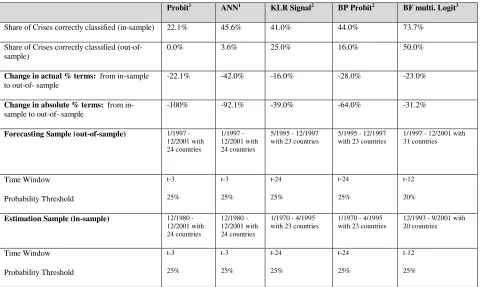
What Poltenen (2006) did not discuss is quantitatively how differently the models preformed from the in-sample to the out-of –sample results. Table 5 below examines this difference:

Table 5: A closer look at the Differences between in-sample and out-of-sample results

Probit1 _ANN1 _{KLR Signal}2 _{BP Probit}2 _{BF multi. Logit}3

Share of Crises correctly classified (in-sample) 22.1% 45.6% 41.0% 44.0% 73.7%

Share of Crises correctly classified (out-of-sample)

0.0% 3.6% 25.0% 16.0% 50.0%

Change in actual % terms: from in-sample to out-of- sample

-22.1% -42.0% -16.0% -28.0% -23.0%

Change in absolute % terms: from in-sample to out-of- in-sample

-100% -92.1% -39.0% -64.0% -31.2%

Forecasting Sample (out-of-sample) 1/1997 - 12/2001 with 24 countries

1/1997 - 12/2001 with 24 countries

5/1995 - 12/1997 with 23 countries

5/1995 - 12/1997 with 23 countries

1/1997 - 12/2001 with 31 countries Time Window Probability Threshold t-3 25% t-3 25% t-24 25% t-24 25% t-12 20%

Estimation Sample (in-sample) 12/1980 - 12/2001 with 24 countries

12/1980 - 12/2001 with 24 countries

1/1970 - 4/1995 with 23 countries

1/1970 - 4/1995 with 23 countries

12/1993 - 9/2001 with 20 countries Time Window Probability Threshold t-3 25% t-3 25% t-24 25% t-24 25% t-12 25%

Source: Adapted from Table 13 and 14 in Poltenen (2006:34)

As can be seen in Table 5 above, the actual percentage change from the in-sample to the out-of-sample in terms of the share of crises correctly classified ranged from -16.0% to 42.0%. In absolute terms, the percentage drop was much higher, ranging from -31.2% to -100%.

18 For the Probit and ANN models the forecasting period is from 1/1997 to 12/2001 and the estimation period is from 12/1980 to 12/2001, thus the forecasting period covers the last 4 years of the 21 year estimation period. Surprisingly both models had extremely poor results during the forecasting period which included the 1997 Asian Crisis and the 1998 Russian Debt Crisis among others. In the conclusions

Poltenen (2006:22) states, ‘In particular, of the currency crisis of the late 1990s, only the Russian 1998 crisis could have been predicted out-of-sample.’ In most likelihood, the reason could have been due to strong contagion effects resulting from the 1997 Asian crisis. Thus, even though the contagion effect was very strong during the 1997 Asian crisis, none of the countries affected by currency crises in Asia were picked up by either model. The forecasting period was within the estimation period, thus both models seemed to miss the regime shift that took place during that time period.

For the KLR Signal and BP Probit models the estimation period is from 1/1970 to 4/1995 and the forecasting period is from 5/1995 to 12/1997. These two models showed results to the ANN model in-sample, and much better results out-of-in-sample, why? Aside from the reasons mentioned earlier by Poltenen (2006), it should be noted that the Mexican Peso Crisis occurred in December 1994 with the subsequent tequila effect. The effects of contagion were prevalent during the last year and a half out of 25 years in the estimation period. The forecasting period included the 1997 Asian Crisis, thus it is surprising that only 25.0% and 16.0% (KLR Signal and BP Probit, respectively) were identified during this period since in terms of contagion effects it was similar to 1994 Mexican Peso crisis period.

The forecasting period is from 1/1997 to 12/2001 and the estimation period is from 12/1993 to 9/2001 for the BF multiple Logit model. The estimation time period would include the Mexican Peso Crisis in 1994, which is only one year into the estimation period. Also included in the estimation window would be the 1997 Asian Crisis and the 1998 Russian Debt crisis. Thus contagion effects would be particularly prevalent during this time period. The question that needs to be asked here, is the model just predicting contagion effects, especially with a time window of t-12? And this model which performed the best predicted only 50% of the crises during the forecasting period of 1/1997 to 12/2001. This number might be a bit deceiving since it depends which crises the model predicted. For example, the results could be skewed if most of the predicted crises occurred during the 1997 Asian Crisis since that would also point to contagion effects.

Bussière and Fratzscher (2002:7 and 30) in discussing the early warning systems (EWS) models in

general and their BF multiple Logit model state that, ‘We find that in particular the financial contagion

channel has been an important factor in explaining and anticipating currency crises.’

Poltenen (2006:17), states that ‘…the proxy for contagion effect is found to have the largest marginal

effect. Namely, a currency crisis in the same region within three months is estimated to increase the

monthly probability of currency crisis by around 15 percent. Economically, this effect is significant.’ He

also notes that any tests on sub-periods in the 1990s need to account for the contagion effect. And as

stated by Poltenen (2006:18), ‘…that economic fundamentals could statistically better explain the onset of currency crises in the subsample of the 1980s than in the subsample of the 1990s.’

However, in an IMF study titled, ‘Vanishing Contagion?’ by Didier, Mauro and Schmukler (2006) they state that contagion has diminished since the 1990s. They note the example of the 2001 crisis in

19 which rely heavily on contagion for prediction. Good results will become harder to attain. Broader implications are that variables fluctuate in importance over time, thus making it harder to predict.

To show the effects of contagion, Table 6 on the next page has been adapted from Bussière and Fratzscher (2002:31). In their study by Bussière and Fratzscher (2002) performed an out-of-sample forecast on the 1997 Asian Crisis with a model end date of December 1996 (denoted as 1996M12 in Table 6). Further out-of-sample forecasts were performed on the 1998 Crises in Brazil/Russia with a model end date of December 1997 (denoted as 1997M12 in Table 6) and on the 2001 Crises in Turkey/Argentina with a model end date of December 2000 (denoted as 2000M12 in Table 6).

Bussière and Fratzscher (2002:29-30) in discussing these different crisis periods starting with the 1997 Asian Crisis state that, ‘For Indonesia, Malaysia, the Philippines and Thailand, probabilities are above 20%, clearly signalling an imminent crisis. For Hong Kong, Korea and Singapore on the other hand, predicted probabilities reach a more modest 16%. The relative failure to predict the Korean crisis comes from the importance of the level of short-term debt relative to reserves in the unfolding of the crisis. Last,

the model sends two important ‘false-alarms’, or more accurately ‘too early alarms’: the predicted probability of a crisis in Russia and Columbia is very high, whereas these countries were hit by a crisis

only in 1998.’

As can be seen in Table 6 in the next page, Brazil had a predicted currency crisis probability of 36.2% and Russia of 88.1% with both crises happening within 9 to 10 months of the model end date (1997M12).

Bussière and Fratzscher (2002:30) state that, ‘In Russia the short-term debt to reserves ratio had risen above 200%, whereas the real effective exchange had significantly deviated from trend (more than 20%), in the context of negative growth rate. For Brazil evidence of contagion is overwhelming: the exchange rate showed only moderate signs of overvaluation (4%), short-term debt was only slightly above the level of international reserves, and the current account deficit (4% of the GDP) was not in itself worrying. The

contagion variable however rose as high as 20% on the eve of the crisis because of Russia’s turmoil – levels above 20% have been reached only by some of the Asian countries in 1997.’ What is clearly

evident is that the macroeconomic indicators pointed to the crisis in Russia, but in the Brazilian case it mostly due to contagion.

Turkey had a predicted crisis probability of 91.4% and Argentina of 13.4% with Turkey happening immediately and Argentina within 3 months of the model end date (2000M12). Bussière and Fratzscher

(2002:30) state that, ‘The Turkish crisis was unambiguously signalled, as the probability of a currency

crisis reached 91%. In fact the model sent a signal by crossing the 20% line as early as November 1999.

For Argentina, the predicted probability of a crisis in December 2000 was not very high. …The reason

why the model does not call the Argentine crisis is that one of the key underlying causes of the crisis was the large share of government debt servicing and the large premium it had to pay on its debt. Both of these factors are only indirectly captured in our benchmark model. This would provide a rationale for

using an extended EWS model adding a broad variety of variables.’

20

Table 6: Bussière and Fratzscher(2000) Predicted Probabilities of Three out-of-sample Forecasts

Crisis Period

(model end date)

Predicted

(threshold: 20% with date of crisis onset)

False Alarms or Too Early

Crisis Not Predicted and Crisis or Crisis After 1-year

Not Predicted and No Crisis

(Threshold % given for borderline cases)

1997 Asian Crisis

Model End Date: 1996M12

Indonesia 0.480 / 97M8

Malaysia 0.305 / 97M7

Philippines 0.68 / 97M10

Thailand 0.340 / 97M7

Columbia 0.685 / 98 M9

Russia 0.329 / 98M9

Hong Kong 0.164 /98M8

Korea 0.167 / 97M11

Singapore 0.167 / 97M10

Czech Rep 0.141 / 97M5

Brazil 0.121 / 98M10

Chile 0.111 / 98M9

7 Countries

Argentina, China, Hungary, Mexico, Poland, Turkey and Venezuela

Borderline Cases (1) Poland 0.114

1998 Brazil/Russia

Model End Date: 1997M12

Brazil 0.362 / 98M10

Russia 0.881 / 98M9

Chile 0.368 / 98M9

Columbia 0.422 / 98M9

Hong Kong 0.711 / 98M8

7 Countries Czech Rep., Hungary, Indonesia, Korea, Malaysia, Mexico, and Thailand

Borderline Cases(7)

Argentina 0.151 China 0.191 Philippines 0.125 Poland 0.120 Singapore 0.179 Turkey 0.166 Venezuela 0.111 2001Turkey/Argentina

Model End Date: 2000M12

Turkey 0.914 / 2000M12 Mexico 0.555 Argentina 0.134 /2001M3 15 Countries Brazil, Chile, China, Columbia, Czech Rep., Hong Kong, Hungary, Indonesia, Korea, Malaysia, Philippines, Poland, Russia, Singapore, and Thailand

Borderline Cases(1) Venezuela 0.172

Source: Adapted from Table 18 from Bussière and Fratzscher (2002:31) Note: Countries in italics represent possible contagion effects.

21 played in anticipating and predicting crises. Table 6, which is adapted by the author from Bussière and Fratzscher (2002:31), clearly shows the effects of contagion. To make this easier to visualize, the relevant countries are in italics.

All the predicted crisis countries for the 1998 Brazil/Russia out-of-sample (model end date of 1997M12) were either false alarms (Columbia and Russia) or not predicted but close to the 20% threshold (Hong Kong, Brazil, and Chile) in the prior 1997 Asian Crisis out-of-sample (model end date of 1996M12).

The same holds for the 2001 Turkey/Argentina out of sample (model end date of 2000M12). All the countries either predicted (Turkey) or not predicted (Argentina) that had a crisis were also borderline cases in the previous 1998 Brazil/Russia out-of-sample (model end date of 1997M12). As mentioned earlier, Bussière and Fratzscher (2002:29-30) state that the probability of Turkey had passed 20% by 1999M11. Finally, Mexico with a probability of 55.5% (0.555) did not experience a crisis during the 1988 Brazil/Russia out-of sample.

In short, all of the predicted crisis countries for the 1998 Brazil/Russia and the 2001 Turkey/Argentina out-of-samples could be the result of contagion effects. In addition, Mexico was a false alarm in the 2001 Turkey/Argentina out-of-sample.

Finally, the time windows used in the studies above are of interest. The Probit and ANN models used t-3, KLR Signal and BP Probit models used t-24 and the BF multiple Logit model used t-12 for the time window, respectively. Poltenen (2006:19) discusses the predictive ability of models under two scenarios

as follows, ‘On the one hand, the model was considered to successfully signal the crisis if the predicted

probability was above the set threshold value at the timing of the crisis. On the other hand, the model was considered to successfully signal the crisis if the predicted probability was above the set threshold within 3 months (t-3) before the actual crisis. Many earlier studies use these ‘crisis windows’ of 12 or 24

months to ‘improve’ the predictability of models. In addition, in some studies, the sample size has been

reduced only to cover certain crisis windows.’ In short, Poltenen (2006) is stating that a successful signal

can occur if you predict the exact timing of the crisis or the crisis happens within your time window. It is, of course, much easier to have a successful signal if the crisis happens within your time window. Thus, larger time window improve the predictability of models. Table 5 (on page 17), clearly shows that the largest time windows of the models were used in the KLR Signal and BP Probit models at t-24. The next largest time window used was in the BF multiple Logit model at t-12.

This point is further addressed by Bussière and Fratzscher (2002:10) who state, ‘The next crucial issue is

the question of what we are trying to predict: the timing of a currency crisis or merely its occurrence? As the state of the literature on EWS models for financial crisis shows, it is already very challenging to predict reliably whether or not a crisis will occur in a particular country. Therefore, predicting not only whether a currency crisis happens but also the timing of when it will happen is a highly ambitious goal

and has, to our knowledge, not been undertaken so far.’

Conclusions

22 specific time frame. The better results are due to the right model with the right variables at the right time combined with an appropriate crisis window and threshold level. Crisis prediction models not only have a large set of variables to deal with but also must contend with the changing importance of certain variables such as contagion. Finally, when the importance of some variables change, the models are rendered ineffective. Thus, it is not surprising that crisis prediction models tend to perform poorly.

A further complicating factor is the extent of the comparability between financial crises. Financial crisis comparability is difficult to justify due to data issues, contextual factors (institutional, social and political), crisis definitions and other issues. This has implications for a theory of crises and in how governments manage financial crises. By taking the context out, large-N studies have possibly missed important information towards the development of a theory of crises. Thus, qualitative studies which leave the context in might be the answer, either alone or with quantitative studies. Finally, policymakers need to be very cautious when using crisis prediction models due to questionable comparability

assumptions.

Acknowledgements

The author would like to specifically thank Professor Klaus Nielsen, Department of Management at Birkbeck College and Dr Michael Gavridis at the European Business School for their feedback and encouragement. In addition, the author is grateful to participants from the annual PhD Seminar at Birkbeck College for their critical comments.

References

Allan and Gale. 2007. Understanding Financial Crises, Oxford University Press.

Berg and Patillo. 1998. Are Currency Crises Predictable? A Test, IMF Working Paper, WP/98/154, November

Berg, Borensztein, and Patillo. 2004. Assessing Early Warning Systems: How Have They Worked in Practice? IMF Working Paper, WP/04/52, March

Bordo, Eichengreen, Klingebiel, Rose and Soledad Marinez-Peria. 2001. Is the Crisis Problem Growing More

Severe? Economic Policy, Vol. 16, No. 32 (Apr., 2001), pp. 51+ 53-82

Bussière and Fratzscher. 2002. Towards a New Early Warning System of Financial Crises, European Central Bank, Working Paper Series No. 145, May

Canova. 1994. Were Financial Crises Predictable? Journal of Money, Credit and Banking, Vol. 26, No. 1 (Feb., 1994), pp. 102-124

Didier, Mauro and Schmukler. 2006. Vanishing Contagion? IMF Policy Discussion Paper, PDP/06/01

Durlauf and Blume, editors. 2010. Monetary Economic, Palgrave MacMillan.

Jacobs, Bruce I. 1999. Capital Ideas and Market Realities, Blackwell Publishers, Inc.

Kaminsky, Lizondo and Reinhart. 1998. Leading Indicators of Currency Crises, International Monetary Fund, Vol. 45, No. 1 (Mar., 1998), pp. 1-48

23 Lowenstein, Roger. 2002. When Genius Failed: The Rise and Fall of Long-Term Capital Management, Fourth Esate, A Division of HarperCollins Publishers.

Mariano, Gultekin, Ozmucur and Shabbir. 2000. Models of Economic and Financial Crises, Middle East Economic Association - MEEA Journal (Online Journal of Loyola University Chicago, www.luc.edu/orgs/meea), Volume 2, September

Reinhart and Rogoff. 2009. This Time is Different: Eight Centuries of Financial Folly, Princeton University Press.

Poltenen. 2006. Are Emerging Market Currency Crises Predictable? European Central Bank, Working Paper Series No. 571, January