How does access to this work benefit you? Let us know!
More information about this work at: https://academicworks.cuny.edu/gc_etds/3419Discover additional works at: https://academicworks.cuny.edu
This work is made publicly available by the City University of New York (CUNY). Contact: [email protected]
City University of New York (CUNY) City University of New York (CUNY)
CUNY Academic Works
CUNY Academic Works
All Dissertations, Theses, and Capstone
Projects Dissertations, Theses, and Capstone Projects
9-2019
Semi-supervised Regression with Generative Adversarial
Semi-supervised Regression with Generative Adversarial
Networks Using Minimal Labeled Data
Networks Using Minimal Labeled Data
Greg Olmschenk
by
Greg Olmschenk
A dissertation submitted to the Graduate Faculty in Computer Science in partial fulfillment of the requirements for the degree of Doctor of Philosophy, The City University of New York.
ii
©2019
Greg Olmschenk
Adversarial Networks Using Minimal Labeled Data
by
Greg Olmschenk
This manuscript has been read and accepted by the Graduate Faculty in Computer Science in satisfaction of the dissertation requirement for the degree of Doctor of Philosophy.
Professor Zhigang Zhu
Date Chair of Examining Committee
Professor Ping Ji
Date Executive Officer
Hao Tang Jie Gong
Ioannis Stamos Jie Wei
Supervisory Committee
iv Abstract
Semi-supervised Regression with Generative Adversarial Networks Using Minimal Labeled Data
by
Greg Olmschenk
Adviser: Professor Zhigang Zhu
This work studies the generalization of semi-supervised generative adversarial networks (GANs) to regression tasks. A novel feature layer contrasting optimization function, in conjunction with a feature matching optimization, allows the adversarial network to learn from unannotated data and thereby reduce the number of labels required to train a predictive network. An analysis of simulated training conditions is performed to explore the capabilities and limitations of the method. In concert with the semi-supervised regression GANs, an improved label topology and upsampling technique for multi-target regression tasks are shown to reduce data requirements. Improvements are demonstrated on a wide variety of vision tasks, including dense crowd counting, age estimation, and automotive steering angle prediction. With training data limitations arguably being the most restrictive component of deep learning, methods which reduce data requirements hold immense value. The methods proposed here are general-purpose and can be incorporated into existing network architectures with little or no modifications to the existing structure.
For the continual mentorship, guidance, and support throughout this work, I would like to thank my advisor Professor Zhigang Zhu (City College of New York). Most importantly, Professor Zhu provided me with critical feedback, which showed where my research was weakest and kept me on track. Similarly, I would like to thank Professor Hao Tang (Borough of Manhattan Community College) for the extensive guidance given and for providing his support whenever it was needed.
Next, I would like to thank the remaining dissertation committee members, most of whom are offering their feedback and time without receiving anything in return. Professor Jie Gong (Rutgers University) has a focus on infrastructure modeling (among other work), and our collaboration in facility analytics directly led to the crowd analysis portion of this work. Professor Jie Wei (City College of New York) has frequently worked alongside our lab, and a project in his course on Computer Vision and Image Processing led my focus toward semi-supervised training for regression tasks. Professor Ioannis Stamos (Hunter College) is an expert in 3D computer vision, and his course in 3D Photography directed me toward scene analysis with a 3D perspective which played a significant role in this work.
I would also like to thank my research colleagues, especially those from the City College Visual Computing Lab, who have given me feedback and have collaborated in my work.
Finally, I would like to thank my family and friends, especially my parents for their continual support and my partner for enduring my schedule.
vi This work has been supported by various grants, agencies, and companies. This includes three National Science Foundation Awards: EFRI #1137172 from the Emerging Frontiers in Research and Innovation Program, PFI #1827505 from the Partnerships for Innovations Program, and SCC-Planning #1737533 from the Smart and Connected Community Program. They all have played a significant role in both my development in machine learning and in facility analysis for serving people in special needs specifically. Appointments to the U.S. Department of Homeland Security (DHS) Science & Technology Directorate Office of University Programs, administered by the Oak Ridge Institute for Science and Education (ORISE) through an interagency agreement between the U.S. Department of Energy (DOE) and DHS lead to my first regression-based deep-learning projects and played a major role in supporting the crowd analysis portion of this work for security applications. ORISE is managed by ORAU under DOE contract number DE-AC05-06OR23100 and DE-SC0014664. The research was also supported by Bentley Systems, Incorporated, through a CUNY-Bentley Collaborative Research Agreement (CRA), whose focus on facility modeling and digital twins allowed this project to move forward with real-world considerations. Additional travel support was provided by the Defense Intelligence Agency via the Rutgers University Consortium for Critical Technology Studies and by a Doctoral Research Award provided by the CUNY Graduate Center, providing the attendance of conferences to present our work. Computing resources were partially supported by a Microsoft Azure for Research Award.
Contents vii
Notation xi
1 Introduction 1
1.1 Deep Learning and Regression . . . 1
1.2 Semi-supervised Generative Adversarial Networks . . . 3
1.3 Contributions of the Thesis . . . 4
1.4 Thesis Organization . . . 6
2 Background for Semi-Supervised Regression GANs 8 2.1 Generative Adversarial Networks . . . 9
2.2 Semi-Supervised GANs for Classification . . . 14
2.3 Alternative Semi-supervised Regression GAN Methods . . . 17
2.3.1 Explicit label semi-supervised regression GANs . . . 17
2.3.2 Dual-goal GAN for regression . . . 19
2.3.3 Binning regression into a classification task . . . 20
2.4 Obliquely Related Methods . . . 21
3 Motivation of SR-GANs 26 3.1 Benefits of SR-GANs . . . 26
CONTENTS viii
3.1.1 Training with minimal data . . . 26
3.1.2 Generalizability of SR-GANs to new situations . . . 27
3.1.3 Increasing accuracy with existing dataset quantities . . . 27
3.1.4 Improved understanding of GANs . . . 28
3.2 Problems and Proposed Solutions . . . 29
3.2.1 Reformulating GANs for regression . . . 29
3.2.2 Training stabilization . . . 30
3.2.3 Developing generally applicable hyperparameters . . . 30
4 SR-GAN Methodology 32 4.1 SR-GAN Formulation Using Feature Contrasting . . . 32
4.1.1 SR-GAN optimization . . . 33
4.1.2 Gradient penalty . . . 36
4.2 SR-GAN Experiments . . . 38
4.2.1 Loss function and stability analysis on synthetic data . . . 39
4.2.2 Hyperparameter generalization on synthetic data . . . 41
4.2.3 Minimal data training on age estimation, steering angle prediction and crowd datasets . . . 42
4.2.4 Crowd labeling: additional means for improving the performance . . . 43
5 Understanding the Behaviors of SR-GANs Through Polynomial Coefficient Prediction 46 5.1 Polynomial Coefficient Estimation Overview . . . 47
5.1.1 Polynomial coefficient estimation dataset . . . 47
5.1.2 Coefficient estimation experimental setup . . . 49
5.2 Loss Function Analysis . . . 52
5.2.3 Cost multiplier grid search . . . 56
5.2.4 Optimal long trials . . . 59
6 Comparing SR-GANs to DNNs Through Age Estimation 62 6.1 Dataset . . . 63
6.2 Experimental Analysis . . . 66
7 Comparing GAN Methods for Steering Angle Prediction 69 7.1 Related Work . . . 70
7.2 Experimental Analysis . . . 71
8 Applying SR-GANs to State-Of-The-Art Crowd Counting Methods 76 8.1 Related Work . . . 79
8.2 Explicit label GAN Design for Crowd Counting . . . 80
8.2.1 Discriminator . . . 80
8.2.2 Generator . . . 82
8.2.3 Dual optimization goal . . . 83
8.3 Experimental Setup and Results . . . 84
8.3.1 Explicit label GAN experiments . . . 85
8.3.2 SR-GAN experiments . . . 88
9 Crowd label topology and upsampling 95 9.1 Related Work . . . 97
9.2 Inverse k-Nearest Neighbor Map Labeling . . . 99
9.3 MUD-ikNN: A New Network Architecture . . . 103
9.4 Experimental Results . . . 106
CONTENTS x 9.4.2 Impact of labeling approach and upsampling . . . 107 9.4.3 Comparisons on standard datasets . . . 110 9.5 ikNN Maps and the SR-GAN . . . 112
10 Conclusion and Discussion 115
Candidate’s Peer Reviewed Publications 118
a A scalar (integer or real)
a A vector
A A matrix
A A tensor
a A scalar random variable
a A vector-valued random variable
A A matrix-valued random variable
P(a) A probability distribution over a discrete random vari-able
p(a) A probability distribution over a continuous random variable, or over a variable whose type has not been specified
Notation xii a∼P Random variable a has distribution P
Ex∼P [f(x)] or Ef(x) Expectation off(x) with respect to P(x)
U(a, b) Uniform probability distribution over the range from a
to b
N Normal probability distribution with mean 0 and vari-ance 1
a+A For any scalar operator combining a scalar and multi-dimensional value, the operation is applied element-wise to the multi-dimensional value. This treatment of operations is also referred to as broadcasting.
D(x) Discriminator network function forward pass with input
x
Introduction
1.1
Deep Learning and Regression
Deep learning [1], particularly deep neural networks (DNNs), has become the dominant focus in many areas of computer science in recent years. This is especially true in computer vision, where the advent of convolutional neural networks (CNNs) [2] has led to algorithms which can outperform humans in many vision tasks [3]. Today, deep learning plays a primary role in nearly every area which uses machine learning methods.
The most common use of DNNs is for classification tasks. These tasks consist of labeling some form of input data as belonging to one or more discrete categories or classes. For example, a classification task may comprise of applying a label to an image, where the label is the type of animal depicted in the image (e.g., ’dog’, ’cat’). The vast majority of deep learning research is focused on these classification tasks. In contrast, a regression task consists of labeling some form of input data with a continuous value. For example, a regression task may consist of determining the distance from a camera to an object, given an image from the camera. The distance may be any value in the continuous range [0,∞), as opposed to a
CHAPTER 1. INTRODUCTION 2 discrete label in the case of classification. Significantly less deep learning research has been devoted to regression problems as compared to classification problems. While the transition from classification to regression may initially seem to be a trivial extension, the current formulations of many deep learning methods do not lend themselves to use in regression tasks. While it is possible to frame any regression task in terms of a classification task, in practice, this presents several significant problems. For example, to recast a regression task as a classification task, an arbitrary number of classes must be chosen, as a continuous range can be segmented into discrete bins in an arbitrary number of ways. This discretizing of the range imposes a limitation on the precision which can be achieved. However, more importantly, the relative locality of the regression values is discarded when converting to a binning classification problem. Due to the formulation of DNN training cost functions, such a naive classification approach would result in each incorrect class being considered equally as wrong. For example, we can consider a prediction of a real number in the range [0,10) which has been split into 10 discrete classes. Given a true label of 10, a prediction of 8 would produce the same loss as a prediction of 2. This results in a problematic training gradient, as well as encouraging the network to overfit since only the single bin shows any improved predictive capabilities. The smaller the bins become, the more problematic this limitation becomes. Depending on the accuracy required by the application, this binning classification approach may be acceptable, but these problems are more naturally framed as the original regression tasks.
The set of regression tasks encompasses a nearly limitless supply of problems that cannot be solved or would be poorly solved by framing them as classification problems. Some examples include crowd counting estimation [4], weather prediction models [5], stock index evaluation [6], object distance estimation [7], age estimation [8], data hole filling [9], curve coefficient estimation, ecological biomass prediction [10], traffic flow density prediction [11], orbital mechanics predictions [12], electrical grid load prediction [13], stellar spectral analysis [14],
prediction [17], ocean current prediction [18], and countless others. Machine learning has been utilized for each of these tasks. The novel method presented in this work can be generalized to any such regression problem, allowing each of these applications to take advantage of the semi-supervised method discussed below.
1.2
Semi-supervised Generative Adversarial Networks
Within the field of deep learning, there are generative models, and more specifically, generative adversarial neural networks [19]. A generative model is one which learns how to produce samples from a data distribution. In the case of computer vision, usually takes the form of a neural network which learns how to generate images, often with specified characteristics. Generative models are particularly interesting because for such a model to generate new examples of data from a distribution, the model needs to ”understand” that data distribution. Arguably, the most powerful type of generative model is currently the generative adversarial network (GAN) [19, 20]. GANs have been shown to be capable of producing fake data that appears to be real to human evaluators. For example, fake images of objects which a human evaluator can not distinguish from real-world images of those objects.
Beyond the generation of fake data, GANs, using a semi-supervised approach, have been shown to produce better results in discriminative tasks using relatively small amounts of labeled data [21], where equivalent DNNs/CNNs would require significantly more labeled data to accomplish the same level of accuracy. This semi-supervised training allows a model architecture which can learn from unlabeled data in addition to labeled data. As one of the greatest obstacles in deep learning is acquiring or producing the vast amounts of labeled data required to train such models, the ability to train these powerful models with less labeled data is of immense import.
CHAPTER 1. INTRODUCTION 4 While GANs have already shown significant potential in semi-supervised training, they have only been used for a limited number of cases. In particular, they have thus far almost exclusively been used for classification problems. This work generalizes semi-supervised GANs to regression problems. The nature of a GAN makes moving from classification to regression problems non-trivial. Specifically, the two parts of a GAN can be seen as playing a minimax game. The discriminating portion of the GAN has the objective of discriminating between fake and real data in some fashion. However, when the real data is labeled with continuous-valued numbers, deciding on what constitutes a ”fake” labeling is not straight forward. To solve this issue, novel loss functions are required. At the same time, these loss functions need to provide a stable training dynamic between the discriminator and generator. These problems, for which solutions are provided in this work, make semi-supervised GANs in regression problems a challenging area of research.
1.3
Contributions of the Thesis
This work presents the following contributions:
1. A novel algorithm generalizing semi-supervised GANs to regression tasks, the Semi-supervised Regression GAN (SR-GAN).
2. An analysis of optimization rules which allows for stable, consistent training when using the SR-GAN, including experiments demonstrating the importance of these rules. 3. Systematic experiments demonstrating the SR-GAN on three typical real-world
appli-cations of regression – age estimation, steering angle prediction, and crowd analysis, all from real-world images. A comparative analysis of alternative methods is also performed.
an analysis of full label resolution for crowd counting.
For a better understanding of the work, we now provide a more detailed summary of each of the above contributions.
SR-GAN theory. The most important contribution is the generalization of semi-supervised GANs to regression in the form of the SR-GAN. As the primary limitation of deep neural networks is currently data limitations, easing this requirement on the countless existing regression problems is immensely important. In addition to the SR-GAN, as a comparison, this work also explores more naive approaches to regression GANs. The capabilities and limitations of these alternatives are demonstrated, and a theoretical understanding of its limitations is provided. The SR-GAN method is designed to avoid the limitations of the alternatives.
SR-GAN behaviors. While the theoretical solution for applying semi-supervised GANs to regression is provided in the first contribution, there are many factors that need to be addressed for this approach to work in practice. Chiefly, the details of loss functions used in the SR-GAN are analyzed. Several variants, each with their own theoretical justification, are examined and tested. This analysis provides both evidence of the SR-GAN’s robust nature and a way to generalize the choice of hyperparameters used to train the SR-GAN.
SR-GAN applications. Next, this work provides several real-world applications where GANs outperform traditional CNNs and other competing models. Specifically, the SR-GAN was applied to predict the age of individuals from single images, to predict the steering angle of a car based on a single frame of video, and to estimate crowd densities in surveillance footage. The age and steering angle estimation tasks provide real-world applications on which the SR-GAN can be used to reduce the data requirements, while still being simple enough to explain the training properties in detail. In the steering angle estimation, it is demonstrated that the SR-GAN approach performs better than previously proposed GAN methods. The
CHAPTER 1. INTRODUCTION 6 crowd analysis case provides a complex real-world application with immediate use cases and demonstrates the capabilities of the SR-GAN on open problems.
Beyond SR-GAN.In addition to the semi-supervised GAN for regression, two additional improvements are proposed to reduce the number of labeled examples required to train a system: improved label topology and use of full-resolution map labels. While these methods are general-purpose, this work only explores there use in the case of crowd analysis. We also discuss the integration of the SR-GAN into multi-optimization goal networks, where challenges are still present.
1.4
Thesis Organization
The remainder of this thesis will be divided into the following chapters.
First, background information will be discussed in Chapter 2. This will include an overview of the GAN and semi-supervised GAN concepts, early works in applying GANs to regression tasks, and the current state-of-the-art works for the specific applications that the SR-GAN will be demonstrated on.
Next, the motivation for this work will be detailed in Chapter 3. This will include a detailed analysis of the current state of GANs for regression, the limitations of these existing approaches, and the underlying theory explaining why another solution is required.
Chapter 4 will describe the methodology of the SR-GAN. Here a formal mathematical definition of this novel GAN method will be provided as well as an intuitive understanding of the approach.
In Chapter 5, a well-controlled synthesized dataset is defined on which can be tested the properties of the SR-GAN while controlling every aspect of the data. This approach allows us to directly observe the underlying data generating model and compare the output of the generator to it. Additionally, it allows us to artificially control the complexity of the dataset
Chapter 6 provides a simple but real-world application for the SR-GAN, namely, age estimation of an individual given a single image. This application provides a direct under-standing of the theoretical design of the model in a practical implementation. The simplicity allows the details of the model to easily be examined while still tackling a real task. In this chapter, improvements over a standard DNN method are the focus.
Similar to the problem of age estimation, Chapter 7 provides another simple real-world application. In this chapter, the network is given the task of predicting the steering angle of a car given an individual image of the upcoming road segment. This can be seen as a simplified version of the self-driving car problem. It provides yet another demonstration that the SR-GAN is a generalizable method. Here the focus is on the improvements of the SR-GAN over other potential GAN approaches.
Chapter 8 provides a complex, real-world application of the SR-GAN. Here the SR-GAN is used to predict crowd densities from surveillance images. Dense crowd counting is still a challenging problem and an open area of research. It is demonstrated that the SR-GAN model can reduce the data requirements of existing CNN state-of-the-art models, thereby improving accuracy overall. The reduction of data on this application is of immense import, as the manual effort required to annotate this kind of data is significant and error-prone.
Next, Chapter 9 provides additional methods beyond the SR-GAN in which crowd labels, and multitarget regression labels more generally, can be improved. This is achieved by an improved label topology and predictive label upsampling.
Finally, Chapter 10 concludes this work, with a discussion of the overall findings and possible implications.
Chapter 2
Background for Semi-Supervised
Regression GANs
In 2012, a deep convolutional neural network called AlexNet [22] won the ImageNet Chal-lenge [23], a competition measuring image classification accuracy. Since this time, deep learning techniques have been able to outperform traditional computer vision techniques in nearly any task where there is enough data to train the deep learning approaches. Further-more, at the time of this writing, there is not an obvious limitation to capabilities of deep neural networks moving forward, other than the limitations of available training data and computing power. The work proposed here attempts to loosen the former limitation.
The development of generative adversarial networks (GANs) [20] specifically presents a means by which the amount of data required by a deep neural network can be lessened. A technique of using GANs in a semi-supervised fashion, where only a small portion of the dataset has labels, has been proposed and shown to produce high levels of accuracy relative to other methods using the same quantity of labeled data [21]. To better understand how this approach works, we will first give a brief explanation of GANs and then an explanation
The following sections give an explanation of GANs and semi-supervised GANs for classification. These explanations are useful for understanding the workings of the SR-GAN proposed here, but the previously existing methods are not directly applicable to regression, as will be shown.
2.1
Generative Adversarial Networks
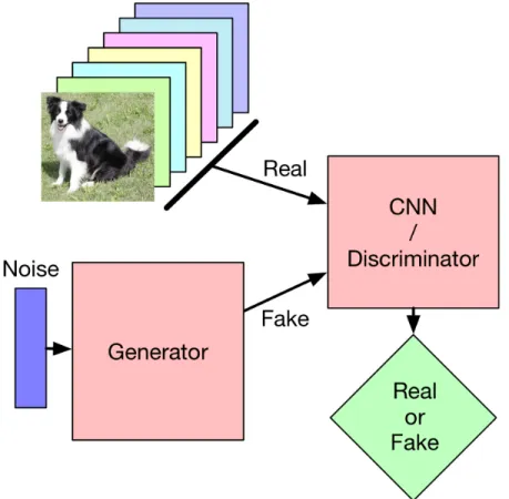
A GAN consists of two neural networks which compete against one another. One of the networks generates fake data; hence, it is referred to as the generator. The other network attempts to distinguish between real data and the fake generated data; consequently, this network is called the discriminator. Both networks are trained together, each continually working to outperform the other and adapting in accordance to the other. In this way, both networks are essentially playing a minimax game [24].
Though GANs are now fairly common, to provide the groundwork for our SR-GAN, it is worth defining the details of a GAN from the viewpoint of probability distributions. First, an intuitive understanding of GANs is provided.
A conventional explanation of the competition between the generator and the discriminator is that of a counterfeiter and a detective. The counterfeiter, the generator, tries to manufacture counterfeit money. The detective, the discriminator, tries to figure out if a given piece of currency is real or fake. In this story, both start with no knowledge but are ready to learn. The generator begins by making a particularly bad example of currency, but as the discriminator is equally bad at determining true currency, it may label the fake example as real money. Here we step in and tell the discriminator it was wrong. The discriminator will then try to find something to help it distinguish between the real and fake data after being told it was wrong. The one remaining twist to the story is that the generator is provided full access
CHAPTER 2. BACKGROUND FOR SEMI-SUPERVISED REGRESSION GANS 10
Figure 2.1: The structure of a basic GAN. Real and fake images are fed to a discriminator network, which tries to determine whether the images are real or fake. A generator network produces the fake images.
to how the discriminator determines which money is fake and which is real. In turn, it changes its counterfeiting approach to find flaws in the discriminator’s new methods. For U.S. currency, the discriminator may first decide that the money needs to have the picture of a person. The generator will learn to make pictures of people. Then the discriminator may realize that it needs to be a specific person on the currency and so the generator will start to learn how to make that specific person’s image. This process continues until both the generator and discriminator become very good at their jobs.
Now for a more formal description. To give a concrete understanding, the remainder of the explanations in this section is given in terms of computer vision problems, specifically where the datasets consist of images. This means an example of real data (and thus the
structure of such a GAN is shown in Figure 2.1.
The generator network takes random noise as input (usually sampled from a normal distribution) and outputs fake image data. The discriminator takes as input images and outputs a binary classification of either fake or real data. Images can be represented by a vector, with each element representing the value of a pixel in the image1. In any image,
each element of this vector has a value representing the intensity of that pixel. For this explanation, a minimum element value (pixel value) of 0 is used, and a maximum of 1 is used. Of course, this vector can be represented as a point in N dimensional space, where
N is the number of elements in the vector. The possible positions of an image’s point are restricted to the N dimensional hypercube with a side length of 1. Here, it is important to note that real-world images are not equally spread throughout this cube. That is, most points in the cube correspond to images that would look like random noise to a human. Images from the real world usually have properties like local consistency in both texture and color, logical relative positioning of shapes, etc. Real-world images lie on a thin manifold within the cube [25]. Subsets of real-world images, such as the set of all images containing a dog, lie on yet a smaller manifold. This manifold represents a probability distribution of the real-world images. We can view the real world as a data generating probability distribution, with each position on the manifold having a certain probability based on how likely that image is to exist in the real world.
The goal of the generator is then to produce images which match the probability distribu-tion of the manifold as closely as possible. Input to the generator is a point sampled from the probability distribution of (multidimensional) random normal noise, and the output is a point in the hypercube—an image. The generator is then a function which transforms a
1One element per pixel is in the case of grayscale images. For RGB images, there are three elements in the vector for each pixel, one for each color channel of the pixel.
CHAPTER 2. BACKGROUND FOR SEMI-SUPERVISED REGRESSION GANS 12
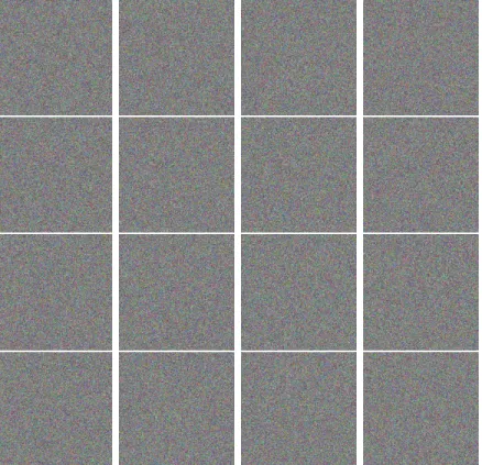
Figure 2.2: An intuitive display that real-world images are not uniformly distributed in image space. Each of the above images was randomly generated, and none show any semblance of structure that we expect to see in a real-world image. Real-world images almost always have some sort of structure or consistency to them (such as nearby pixels often having similar values).
normal distribution into an image data distribution. Formally,
pf ake(x) =G(N) (2.1)
where G represents the generator function, x is a random variable representing an image, N is the normal distribution, andpf ake(x) is the probability distribution of the images generated by the generator. The desired goal of the generator is to minimize the difference between the generated distribution and the true data distribution. One of the most common metrics to minimize this difference is the Kullback-Leibler (KL) divergence between the generator distribution and the true data distribution using maximum likelihood estimation. This is
θ∗ = arg min
θ
DKL(pdata(x)kpf ake(x;θ)). (2.2)
To find this set of parameters, each of the discriminator and the generator works toward minimizing a loss function. With Dbeing the discriminator’s inference function, the discrimi-nator’s loss function is given by
LD =−Ex∼pdata[logD(x)]−Ex∼pf ake[log(1−D(x))] (2.3)
and the generator’s loss function is given by
LG =−Ex∼pf ake[log(D(x))]. (2.4)
For each network, the derivative of their respective losses are used to update the network parameters via the backpropagation algorithm. In the case of image data, this approach has led to generative models which can produce realistic looking images reliably [26].
However, this type of GAN does not improve the capabilities of the discriminator on any predictive task. Here, the discriminator is only used to train the generator. This can be understood further if we assume an ideal discriminator and generator network. In this case, the generator would eventually learn to produce data which exactly matches the data distribution of the real data, or, in the case of limited training data, produce images which exactly match those in the training dataset. In this case, the best prediction the discriminator can give is a 50% probability that the image is a real image.
CHAPTER 2. BACKGROUND FOR SEMI-SUPERVISED REGRESSION GANS 14
2.2
Semi-Supervised GANs for Classification
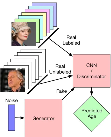
In this section, a subset of GANs is explained which are used to improve the training of neural networks for discrimination and prediction tasks. Specifically, this type of GAN allows a predictive network to train with less labeled data using a semi-supervised approach. In this case, both a labeled and an unlabeled dataset are used. In addition to distinguishing between real and fake data, the discriminator also attempts to label real input data into one of the real world classifications. The primary goal of this type of GAN is to allow the discriminator’s prediction task to be trained with relatively small amounts of labeled data using unlabeled data to provide the network with additional information. As unlabeled data is usually much easier to obtain than labeled data, this provides a powerful means to reduce the requirements of training neural networks. This semi-supervised GAN structure can be seen in Figure 2.3.
Where in a simple GAN the discriminator would be passed true examples and fake examples, in the semi-supervised GAN the discriminator is given true labeled examples, true unlabeled examples, and fake examples. We can better understand why this is useful by considering the case of image classification. In this case, the discriminator is being trained to predict the correct class of a true image, which can be one of the K classes that exist in the dataset. The discriminator is given the additional goal of attempting to label any fake images with a K+ 1th class, which only exists to label fake data (i.e., does not exist in the true label dataset). For the case of unlabeled, all we know is that it must belong to one of the first K classes, as the K+ 1th class does not exist in the real data. The discriminator is then punished for labeling true unlabeled data as the K+ 1th class. This is useful because the discriminator cannot simply overfit to the labeled data, as it still has to accommodate for the unlabeled data. At the same time, the fake data prevents the discriminator from allowing simple features to be the deciding factor, as the generator is able to produce such simple
unlike ordinary forms of regularization, this regularization is based on the distribution of the data.
To understand what is happening in this semi-supervised learning more intuitively, we can start with a non-GAN classification network. Such a network learns a transformation function which partitions image space into separate classes. The network can only learn from the labeled data and warps its partitions to best fit each of the labeled classes into the partition they belong to. At this point, adding unlabeled data to the training process provides no additional benefit. There is currently no constraint on the extent of the classification partitions (except at the boundary of another class), and so all unlabeled data will lie within one of the class partitions. As the new data is unlabeled, this provides no additional information. It is only with the additional cost of the fake class that the unlabeled data can be used with any value. Once the fake data narrows the range of the partitions, we can see them as manifolds once again. Now there are few labeled data points and many unlabeled data points, all of which must lie on the manifolds of the real classes. The manifolds have different regions (or even separate manifolds) for each class, but even the unlabeled data has to lie somewhere on the manifold(s). As the discriminator trains, it learns how to segment the data points into categories. To do this, it creates a mapping from a predictive manifold to a class, with the training warping the manifold to contain each of the data points for that class. At the same time, the generator prevents the manifold from warping too severely to reach data points in arbitrary ways. Intuitively, this is because severely warping the manifold to reach true data points can result in the manifold stretching into the area which does not represent true images. The generator acts a pressure on the manifold to reduce this. By generating images near the manifold, the generator forces the discriminator’s manifold not to wander into areas that don’t contain real images. In this sense, the generator is a form of regularization for the discriminator, but one which is based on real-world data. At the same
CHAPTER 2. BACKGROUND FOR SEMI-SUPERVISED REGRESSION GANS 16 time, the unlabeled data forces the manifold to reach as much of the real data distribution as possible. In doing so, the discriminator must learn enough robust and complex features to reach all the real data while not learning arbitrary overfitting features that stretch the manifold into the fake regions.
As originally formulated by Salimans et al. [21], the semi-supervised GAN’s discriminator loss function is then defined by
LD =Lsupervised+Lunsupervised (2.5)
Lsupervised=−Ex,y∼plabeledlog[D(y|x, y < K+ 1)] (2.6)
Lunsupervised =
−Ex∼punlabeledlog[1−D(y=K+ 1|x)]
−Ex∼pf akelog[D(y=K+ 1 |x)].
(2.7)
As for the generator, the first option for a loss function is the straight forward one which aims to have the discriminator label the fake images as from real classes. Specifically,
LG =−Ex∼pf akelog[D(y < K+ 1 |x)]. (2.8)
However, Salimans et al. [21] achieved improved results by training the output activations of an intermediate layer of the discriminator have similar statistics in both the fake and real image cases. That is, the generator should attempt to make its images produce similar features in an intermediate layer (instead of final classification output) as is produced when true images are input. This can be intuitively understood as making the statistics of the
used in deciding a classification. The simplest and most useful statistic to try to match is the expected value for each feature. Formally put, if we denote f(x) as the features output by an intermediate layer in the discriminator, then the loss function for the generator becomes
LG= Ex∼prealf(x)−Ex∼pf akef(x) 2 2. (2.9)
This benefits the process by preventing the generator from producing images which exactly match those from the real training dataset. If the generator learns to produce exactly images from the training data, the generator provides no new information not gained from the training data itself. Instead, the feature matching goal encourages the generator to produce images from the same image distribution, but not specifically the same images.
Since their development, semi-supervised GANs have been used to improve training in many areas of classification, including digit classification [27, 28, 21], object classifica-tion [27, 28, 21], facial attribute identificaclassifica-tion [28], and image segmentaclassifica-tion (per pixel object classification) [29].
2.3
Alternative Semi-supervised Regression GAN
Methods
2.3.1
Explicit label semi-supervised regression GANs
While we have defined why this is an important area to research, it has not yet been explained why this task would require any great effort. Why can we not simply take our solution for classification and apply it to a regression problem?
CHAPTER 2. BACKGROUND FOR SEMI-SUPERVISED REGRESSION GANS 18 classification semi-supervised GAN (Equations (2.5) to (2.7)). These functions call for the labels to belong to a specific class, whether it be one of the real classes or the generated fake class. Obviously, regression problems do not have classes. The discriminator desires the labeled examples to be given the correct class, the unlabeled examples to be given any existing real class, and the fake examples to be given a new fake class. For regression tasks, the labeled case is still straight forward: the discriminator is trained to minimize the error between its predictions and the true labels. The goal of the discriminator for the unlabeled examples and the fake examples is less clear. The first option would be to have the discriminator distinguish between real and fake data using the predicted regression value. Yet, which values to choose for what constitutes real data and what constitutes fake data is challenging.
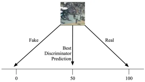
In many applications, the possible real data values may be in the range (−∞,∞), in which case, there is no option left for a fake label value. Even if we dismiss this limitation, other significant issues still arise. Most notably, using an explicit label range to constitute a fake label results in a prediction bias. For example, we can consider the case of crowd counting, where the goal is to predict the number of people in a given image. Here, the possible true values are in the range [0,∞). We might then choose to make a negative number constitute a fake label. In the case of an ideal generator, the generator would learn to produce exactly images from the real dataset. The ideal discriminator then has a dilemma. The same image may have come from the real data or the generator. In the former case, it should predict the correct count, while in the latter case, it should predict a negative number. In this situation, the discriminators best choice is to predict half the correct count of the real image. Since the overall goal of the semi-supervised GAN is to improve the predictive powers of the discriminator, this produces an undesired bias. This scenario is depicted in Figure 2.4. Of course, the generator will never perfectly produce duplicates of the real data, but a significant bias effect is still present in this model.
range of the real labels is not known. Rezagholiradeh and Haidar [30] presents such an explicit label GAN, which is compared against the proposed SR-GAN method in the driving steering angle experiments.
2.3.2
Dual-goal GAN for regression
Another potential alternative to the proposed method is a dual goal GAN (DG-GAN) approach. A DG-GAN outputs two labels: a regression value prediction and a fake/real classification prediction. The idea is that the network must learn both how to distinguish between real and fake examples, and how to predict the correct value for a labeled example. However, this approach also has several potential flaws. First, the method does not enforce that these two prediction goals be related. Part of the network may learn the task of identifying real/fake images, while another portion of the network learns the task of predicting regression values. A representation of this split learning is shown in Figure 2.5. If the objective of distinguishing being real and fake examples is weighted strongly enough, the network may devote larger portions of the network to the real/fake classification task, thereby reducing its effectiveness in the regression prediction.
Additionally, this approach presents a bias similar to the one encountered using the explicit label model. Specifically, two linear transformations are used from the final feature vector to produce the regression value and the real/fake classification. Although the two predictions undergo different non-linear activation functions (a linear activation for the regression value and a sigmoid activation for the real/fake classification), the values entering these activation functions are linearly dependent. The bias here is mitigated by the non-linear activation, but each feature is linked to both output values with a static weight (after training). Once again, certain regression values are considered more real than others, leading to a bias in the predicted values.
CHAPTER 2. BACKGROUND FOR SEMI-SUPERVISED REGRESSION GANS 20
2.3.3
Binning regression into a classification task
Finally, it is possible to simply reformulate any regression task into a classification task by binning the regression values into discrete bins. In practice, this presents several significant problems. For example, to recast a regression task as a classification task, an arbitrary number of classes must be chosen, as a continuous range can be segmented into discrete bins in an arbitrary number of ways. This discretizing of the range imposes a limitation on the precision which can be achieved; Using the center value of the bin as the predicted value, the average error for any value within the bin is 14 the size of the bin. As the bins become larger, the greater the precision limitation of the bin.
More significantly, the relative locality of the regression values is discarded when converting to a binning classification problem. The usual softmax loss for multiclass tasks results in each incorrect class bin being considered equally as wrong. For example, we can consider a prediction of a real number in the range (0,100) which has been split into 4 discrete classes. Given a true label of 95, a prediction of the (50,75) bin would produce the same loss as a prediction of (0,25). Firstly, this results in a problematic training gradient, as any nearby bins are considered entirely wrong, and moving from a far bin to a close, but wrong, bin does not produce a lower loss. Without this training information, the network may stall in improvements. Furthermore, it encourages networks which overfit, since only the single bin improves the loss, and a solution which moves many values closer to their correct bin will be ignored for one that increases the weight of an already near correct prediction. These problems are depicted in Figure 2.6. The smaller the bins become, the more problematic this limitation becomes. Loss functions which take into account locality of bins are significantly more inefficient and impractical for use in neural network training.
2.4
Obliquely Related Methods
Zero/one/few-shot learning methods [31] and other meta/transfer learning methods [32] have been rapidly developing in the last few years. These methods seek a similar end goal as the semi-supervised GAN approach: provide a network which functions well on a task with little labeled data for the task. However, the method by which they approach the problem is significantly different. Few-shot methods focus on learning a separate task from the final goal, then work to use those learned transformations on for the new task. The semi-supervised GAN approaches only includes data from the desired task but takes advantage of learning from unlabeled data.
These two approaches are complementary rather than competing approaches. Zhang et al. [33] uses a semi-supervised GAN on top of a few-shot method to demonstrate further improvements. In particular, Zhang et al. [33] shows that this approach generalizes to most few-shot models. Beyond the complementary nature, few-shot approaches are even newer than semi-supervised GANs, are (currently) typically applied to simpler applications than semi-supervised GANs, though this may change in the near future.
Similar to the case of semi-supervised GANs, these few-shot approaches are almost exclusively applied to classification rather than regression tasks. Given all these factors, few-shot learning and meta-learning approaches are not relevant enough to the method proposed here to be included in this work.
Another distinct category of related work is that of regression in conditional GANs. Conditional GANs are a type of GAN designed to produce realistic examples which have specific desired properties in the example. Bazrafkan and Corcoran [34] provides an approach to generate images with specific characteristics in a conditional GAN. In particular, they use a regressor in parallel with the discriminator network to provide more variation in the generated examples. These works are attempting to produce realistic-looking generated
CHAPTER 2. BACKGROUND FOR SEMI-SUPERVISED REGRESSION GANS 22 examples. The product is not a predictive network for real examples.
In contrast, our approach is designed to improve the predictive capabilities of the discrim-inator on real examples. Notably, we do not expect our generator to produce realistic-looking examples. On the contrary, we expect the examples generated will not look realistic. As noted by Salimans et al. [21], the use of feature matching (which is also used in our work) improves the discriminator’s predictive accuracy while reducing the realism of the generated examples. We expect our feature contrasting approach further erodes the realism. Furthermore, works such as Dai et al. [35] show how a generator which produces examples that are too realistic may be less advantageous for improving a discriminator’s predictive abilities.
Figure 2.3: The structure of a semi-supervised GAN. Both labeled and unlabeled real images, as well as fake images, are fed to a discriminator network, which tries to determine which class each image belongs to (K real classes and one fake class). The discriminator wishes to label images from the generator as belonging to a special ”fake” class.
CHAPTER 2. BACKGROUND FOR SEMI-SUPERVISED REGRESSION GANS 24
Figure 2.4: A prediction bias is introduced when using an explicit fake label range for regression values. In crowd counting, true values are in the range [0,∞), so negative values may represent the fake label. However, if a generator can produce images which exactly match the real image distribution, the best prediction the discriminator can pick is half the value. Here, an image containing 100 people could be either from the real data or the hypothetical perfectly trained generator. In this case, the discriminator’s best prediction is 50. This results in an extreme prediction bias, and does not improve the predictive capabilities of the discriminator for crowd counting.
Figure 2.5: A DG-GAN network splitting the network into solving the two objectives inde-pendently, rather than using a shared representation. The dashed lines represent connections which exist but have very low weights. The degree of this division of learning can vary.
Figure 2.6: Reframing a regression problem as a classification task by binning regression values has two major limitations. First, the bin size limits the precision of the prediction. This problem becomes more significant as the larger the bins become. Second, applicable loss functions do not consider the locality of the bins. This results in several significant training limitations. This problem becomes more severe as the smaller the bins become.
Chapter 3
Motivation of SR-GANs
3.1
Benefits of SR-GANs
The main advantage of the SR-GAN is the reduction of data for training a network. However, this manifests itself in three important ways: 1) Networks can be trained in cases where not much data is available, or large amounts of effort are required to annotate data. 2) Training can be easily generalized to new situations, as little or no new annotated data is needed from that specific situation to train the network to it. 3) Models for existing datasets can be trained to higher accuracies with the SR-GAN than would be possible with the traditional network alone.
3.1.1
Training with minimal data
In the case of the MNIST handwritten digits dataset [36], Salimans et al. [21] found that 99% accuracy could be achieved with only 100 training images using semi-supervised GANs, wherewith a standard CNN it would take around 10,000 to achieve the same level of accuracy. This reduction of data requirements is one of the primary reasons we wish to expand on this
Most current deep learning implementations are limited only by a lack of data or lack of time or computing resources to train the networks. That is, for most well-defined problems, if we were provided a virtually limitless supply of data and time, the existing neural network formulations could solve the problem. However, in most cases data is limited, often severely so. The SR-GAN works to expand these capabilities to regression tasks. Expanding the range of problems a semi-supervised GAN can apply to allows a way to solve the issue of limited data in more applications, and this is the primary benefit of the SR-GAN.
3.1.2
Generalizability of SR-GANs to new situations
Another reason semi-supervised GANs are compelling is one that arises implicitly from needing less data. Specifically, it presents networks which are able to generate new examples and compares them against its own predictions. That is, being able to abstract new instances from the idea of an example rather than merely trying to learn a simple representation to fit every example in the training dataset. This process of generating new versions of the thing being learned, and comparing them against real examples to look for inconsistencies forces the GAN to learn more robust and complete representations. Although perhaps speculative, this may be leading neural networks closer toward how human brains are able to learn ideas with fewer examples.
3.1.3
Increasing accuracy with existing dataset quantities
Ideally, for training deep neural networks, the network would have access to an unlimited supply of annotated data. Of course, producing such data is impractical or impossible. Instead, if a network cannot be designed which can reach the level of accuracy the developer requires, then more data is typically annotated. Once the required accuracy is reached, often,
CHAPTER 3. MOTIVATION OF SR-GANS 28 there is not much incentive for the developer to annotate more data. However, if more data would allow the network (or a more powerful network) to perform the task even better than we expect the SR-GAN would help improve the results with the current level of data.
On the other hand, we expect a limitation to the benefit of the SR-GAN. In the best case, as the quantity of annotated data approaches infinity, we should expect that the SR-GAN would provide no benefit, as labeled data can always provide more information than unlabeled data used in a clever way. Furthermore, we can expect that, if imperfectly designed, the SR-GAN would actually be a determent to accuracy when the amount of annotated data approaches infinity. This is because the SR-GAN encourages the network to minimize a loss which is not directly being trained for. If there is unlimited annotated data, training only for the primary task should yield the best possible results, and the SR-GAN introducing a new goal can at best do nothing, but may also encourage the network to move away from the ideal network. If there is no chance the quantity of data available would lead to this, then this isn’t an issue. However, if we want to make the SR-GAN generalized to work in every case, even cases where extremely large quantities of the labeled data is available, this issue needs to be taken into account. Luckily, the real-world experiments presented in this work did not encounter this issue. This suggests that the detriment of using the SR-GAN in problems with large amounts of labeled data is negligible.
3.1.4
Improved understanding of GANs
While the above generally explains why it is interesting to investigate GANs and semi-supervised GANs in more detail, there are also specific reasons for semi-semi-supervised GANs for regression problems.
Firstly, there are countless problems which require the use of a regression method to be solved. The crowd analysis case described in this work is one such example. Beyond the methods described in Section 2.3, the solutions for classification problems currently handled
SR-GAN avoids the problems and limitations of the methods from Section 2.3.
More importantly, semi-supervised GANs for regression are interesting because regression is more general than classification. Specifically, classification is a subset of regression. In particular, any classification problem can be framed as a regression problem. The typical formulation of a neural network is to output a continuous number as a ”score” for each class, and simply choose the highest score to be the predicted class. The SR-GAN methods can be applied directly to this output, or the following loss function (typically from a softmax) without any issues. This is not true of converting from regression to classification, as described in Section 2.3.3. Classification can be considered a subset of regression problems, and any of the solutions used for general regression can be applied to classification. As such, this work helps expand the overall application and understanding of semi-supervised GANs.
3.2
Problems and Proposed Solutions
While we have defined why this is an important area to research, a complete reasoning of why this is a challenging task needs to be expounded.
3.2.1
Reformulating GANs for regression
The first major issues have already described in the limitations of alternative semi-supervised regression GAN models in Section 2.3. Namely, how to formulate the mathematics of the semi-supervised regression GAN so as not to introduce biases or other training issues. Converting the problem to a binned classification problem leads to both precision and limited training issues. An explicit fake label method leads to significant prediction bias. The DG-GAN method leads to split goal network training and additional biases. So the first issue to solve is in developing a mathematical formulation of the SR-GAN which does not introduce these
CHAPTER 3. MOTIVATION OF SR-GANS 30 problems or others. Such a formulation is provided in Chapter 4.
3.2.2
Training stabilization
A major challenge in training any type of GAN (not exclusively an SR-GAN), is building the network cost that reliably converges [37]. Particularly in the case of the proposed SR-GAN method (see Chapter 4), the possible choices of loss functions present several ways where the training between the discriminator and the generator could oscillate or otherwise fail to converge.
Several methods have been suggested as to how to stabilize GAN training for the case of classification. Throughout this work, we use a gradient penalty method [37] to dampen and converge generator/discriminator oscillation. However, this dampening is only applicable if the model is only failing to converge due to training oscillation. If the semi-supervised loss functions are inherently unstable, no amount of dampening would resolve the problem. While there are countless choices of unstable loss function combinations, choosing a stable set is relatively simple once the details are understood. Furthermore, the experiments in Chapter 5 demonstrate that the choice of loss functions is relatively unimportant to the resulting accuracy, so long as a stable set of loss functions is chosen.
3.2.3
Developing generally applicable hyperparameters
While the accuracy of neural networks is arguably the most crucial reason they are so widely used today, another highly important reason is their generalizability. Within computer vision, well-known networks such as AlexNet [22] and VGGNet [38] have been used for countless specific applications with little or no change to the existing network structure. Much of the success of neural networks stems from their ability to require little change to function in a new setting. Earlier networks often had difficulty converging or would take too long to train
with more complex optimizers like the Adam optimizer [39], have allowed neural networks to provide a working solution with far less application-specific hyperparameters.
In a similar fashion, the SR-GAN requiring many handcrafted hyperparameters for a single application is not desirable. We wish to obtain a model which will function over a wide range of scenarios with little or no change to the main SR-GAN algorithm or hyperparameters. In particular, how to weigh the relative values of the various supervised and unsupervised optimizations initially seems to be a daunting task. However, in Chapter 5, it is demonstrated that the choice of weighting the various components is quite forgiving, so long as a few generalizable guidelines are followed.
Chapter 4
SR-GAN Methodology
4.1
SR-GAN Formulation Using Feature Contrasting
The semi-supervised regression GAN (SR-GAN) approaches regression estimation by com-paring the types of available data (labeled, unlabeled, and fake) as probability distributions rather than individual examples. In this method, the discriminator does not attempt to predict a label for the unlabeled data or fake data. Instead, the statistics of the features within the network for each type of data are compared. Here is the fundamental idea: We have the discriminator seek to make the unlabeled examples have a similar feature distribution as the labeled examples. The discriminator also works to have fake examples have a feature distribution as different from the labeled examples distribution as possible. This forces the discriminator to see both the labeled and unlabeled examples as coming from the same distribution, and fake data as coming from a different distribution. In this way, it learns to distinguish between the different distributions of the examples rather than distinguish individual examples as real or fake. The generator, on the other hand, will be trained to produce examples which match the unlabeled example distribution, and because of this, the
drawn from that distribution is still decided based on the labeled examples (as it is in ordinary DNN/CNN training), but the fact that the unlabeled examples must lie on the true example distribution manifold forces the discriminator to more closely conform to the true underlying data generating distribution. At the same time, avoiding the fake distribution prevents the discriminator from stretching the prediction manifold away from the true data distribution.
4.1.1
SR-GAN optimization
The SR-GAN structure is shown in Figure 4.1 with the age estimation application depicted as an example. The method for matching the features of two types of data was initially proposed in Salimans et al. [21]. Salimans et al. [21] used the method to train the generator to avoid generator mode collapse. We also use the feature matching to train the generator to match the fake and unlabeled data. However, we also extend the feature matching to the case of training the discriminator to match the two real data distributions (labeled and unlabeled). In the case of training the discriminator to distinguish between the unlabeled distribution and fake distribution, we propose a novel approach,feature contrasting, which is antithetical to feature matching. In this case, the discriminator attempts to make the features of the real and fake data as dissimilar as possible, while the generator is attempting to make these features as similar as possible.
Specifically, the loss functions as defined for the semi-supervised GAN for classification (Equations (2.5) to (2.7)) are entirely reformulated in the case of regression. First, we separate
the loss of the discriminator into several terms for clarity. This is given by
LD =Lsupervised+Lunsupervised
=Llabeled+Lmatching +Lcontrasting
CHAPTER 4. SR-GAN METHODOLOGY 34 What we refer to as the ”labeled loss”, is given by
Llabeled =Ex,y∼pdata(x,y)[(D(x)−y)
2]. (4.2)
This loss is similar to an ordinary fully supervised loss (for regression training). Next, the ”matching loss” causes the discriminator to attempt to make the feature statistics of the real labeled data and the real unlabeled data be as similar as possible. This matching loss is given by
Lmatching =kEx∼plabeledf(x)−Ex∼punlabeledf(x)k
2
2. (4.3)
In contrast, the ”contrasting loss” causes to the discriminator to attempt to make the feature statistics of the real data as dissimilar to the fake data as possible. Withf(x) being a feature vector within the network given inputx, this feature contrasting is accomplished with the loss function given by
Lcontrasting =−
log |Ex∼pf akef(x)−Ex∼punlabeledf(x)|+ 1
1. (4.4)
Finally, the generator attempts to make the feature statistics of the real data match those of the fake data. This goal is accomplished by the generator loss given by
LG =Ex∼pf akef(x)−Ex∼punlabeledf(x)
2
2. (4.5)
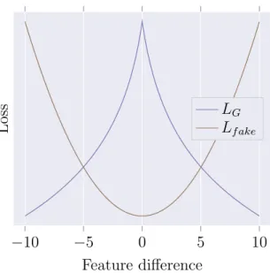
Here, Lmatching and LG are identical except in which data distributions are being compared. Additionally, the feature contrasting in Equation (4.4) is in direct opposition to the feature matching in Equation (4.5). Notably, there is no possibility for the generator and discriminator to both benefit by a change in one of the features; A decreased loss for one necessarily results an increased loss for the other (for the change in an individual feature difference). A comparison
the functions used to measure the distance between the two distributions can vary, and the choice of these loss functions are discussed in more detail in Chapter 5.
Notably, the matching and contrasting functions for the two distributions need to provide conflicting goals for any given feature difference to prevent the discriminator and generator from converging. Additionally, it is important to note that the derivative of the loss function is the value which the neural network is actually trained on. The contrasting function cannot simply be the negative of the matching function. Where the matching function has little slope near zero, the contrasting function should have the largest slope near zero. Intuitively, the largest desire to create an increased contrast occurs when the distributions to be contrasted are exactly matching. For matching, the further the two distributions are apart, the greater the need to make them match. If the contrasting slope were to increase (rather than decrease) further from zero, there is the potential for a runaway training gradient.
To summarize, the SR-GAN uses feature matching for the discriminator loss functions where in previous methods a separate ”fake” class is defined. Specifically this can be seen in the change from the unsupervised loss in Equation (2.7) (which uses a ”fake” class in the discriminator) to Equations (4.3) and (4.4) (which uses feature layer statistics). This accomplishes several goals:
1. Regression problems have no classes, and the previous methods require a ”fake” class definition, and the SR-GAN approach allows regression problems to be approached. 2. The feature statistics comparison does not introduce any bias in the discriminator label
prediction, as the final label output is not used in the unsupervised loss.
3. The feature statistics comparison uses every feature of a layer in its comparison. 4. The approach requires no prior information about the data and requires no manual
CHAPTER 4. SR-GAN METHODOLOGY 36 Notably, the above points solve the issues with the alternative models in Section 2.3. Firstly, no arbitrary binning is required, with the training goal is the original regression goal.
Next, the final output label is not used as part of the unsupervised loss. In particular, a change in the labeled, unlabeled, and fake distributions does not require a change in the output regression values; statistically different feature vectors can produce the same regression value, resulting in optimization option which does not introduce a bias in the regression prediction.
Where the DG-GAN can split the model into achieving two separate goals, the SR-GAN cannot. Unlike in the DG-GAN, every value in the SR-GAN’s feature vector is included in distinguishing between real and fake distributions; since there is no benefit to splitting the model, all values are used in the regression prediction. This is depicted in Figure 4.3.
Finally, both the explicit fake label GAN and the binning classification GAN require manually setting hyperparameters, requiring expert domain knowledge. The SR-GAN requires no such information and automatically distinguishes between distributions.
4.1.2
Gradient penalty
An additional challenge preventing the use of an SR-GAN is the difficulty of designing an objective which reliably and consistently converges. GANs can easily fail to converge under various circumstances Barnett [40]. To solve these general GAN instability issues, we use the gradient penalty approach proposed by Arjovsky, Chintala, and Bottou [41] and Gulrajani et al. [37].
The gradient penalty as defined by Gulrajani et al. [37] is not applicable to our situation, because their gradient penalty is based on the final output of the discriminator. As the final output of the discriminator is not used in producing the gradient to the generator, we use a modified form of the gradient penalty. This gradient penalty term is added to the rest of the
L=Llabeled+Lmatching+Lcontrasting +λEx∼pinterpolate max k∇xˆ(f(x))k22−1 ,0 . (4.6) where pinterpolate examples are generated byαpunlabeled+ (1−α)pf ake for α ∼ U, and λ
being a manually chosen scalar. The last term provides a restriction on how quickly the discriminator can change relative to the generator’s output. Our version of the gradient penalty term is modified in multiple ways from the original. First, as noted above, the final discriminator output cannot be used, nor should it, as the discriminator’s interpretation of the generated data only matter in regard to the feature vector,f(x). Second, the gradient penalty is normally applied to a term similar to the Lcontrasting term using the interpolated values, as this value is related to how the discriminator views the generator’s data. However, our
Lcontrasting is based on the average of a batch of fake examples whose difference is then taken
from a batch of real examples. As both the Lcontrasting term and interpolates are calculated
based on the real data, the resulting gradient penalty is negligible. Instead, we apply the gradient penalty directly to the mean feature vector of a batch of interpolated examples and do not apply the feature distance loss function compared to the mean real feature vector. As this penalizes the gradient even for mean feature vectors far from the mean real feature vector, it may slow training. However, near the real feature vector, it approximates the original gradient penalty formulation and works well in practice. Lastly, we use the one-sided version of the gradient penalty described by Gulrajani et al. [37]. As mentioned in their work, the one-sided penalty more closely matches the desired discriminator training properties, and we found this approach to produce higher accuracies than the two-sided penalty.
CHAPTER 4. SR-GAN METHODOLOGY 38
4.2
SR-GAN Experiments
To demonstrate the capabilities of the semi-supervised regression GANs, we use two experi-mental regimes, each of which consists of several individual trials and demonstrations.
The first experimental regime is of a synthesized dataset problem. This allows us to demonstrate the details of the theory behind a semi-supervised regression GAN in a well-controlled and understood environment. The dataset consists of values taken from randomly generate polynomials. The goal of the network is to predict the original polynomial coefficients based on the sampled data. This data generating distribution is explained in detail in Chapter 5. Using this simple problem, we can show how the semi-supervised regression GAN works in detail, what variations can influence its capabilities, and what its limitations are.
The second experimental regime consists of real-world applications with specific use cases. Three applications, driving steering angle prediction, age estimation and crowd analysis, have been chosen for this purpose. The simplest variant of the crowd analysis case is taking a single image and estimate how many people are in the image. Similarly, the steering angle and age estimation cases result in a single predicted value and are all determined from single images. However, there are more complicated areas we wish to deal with in regard to the crowd counting case, specific, per pixel density labels, and analysis of grouping within areas of the image. Of particular value, having the real-world applications gives meaning to the differences in accuracy between the SR-GAN method, the base DNN method, and the alternative GANs we are examining, and allows for comparisons in the future. Finally, the real-world case provides an area we can show direct improvements in compared to the state-of-the-art of that field.
4.2.1
Loss function and stability analysis on synthetic data
Of the ch