The Impact of Exogenous Asymmetry on Trade and Agglomeration in Core Periphery Model

Munich Personal RePEc Archive

The Impact of Exogenous Asymmetry on

Trade and Agglomeration in

Core-Periphery Model

Sidorov, Alexander

Sobolev Institute of Mathematics SB RAS

2011

Online at

https://mpra.ub.uni-muenchen.de/32826/

The Impact of Exogenous Asymmetry

on Trade and Agglomeration in Core-Periphery Model

Alexander V. Sidorov∗

Sobolev Institute of Mathematics SB RAS, Novosibirsk, Russia

Abstract

The paper studies the Krugman’s CP model in the weakly explored case of asymmetric regions in two settings: international trade and agglomeration processes. First setting implies that the industrial labor is immobile, while second one consider mobile industrial labor and long-run equilibria. An-alytical study of both settings requires application of advanced mathematical analysis, e.g. implicit function theory. For international trade we find how equilibrium prices, production, consumption, wages and welfare for all population groups respond to shifts in all exogenous parameters: character-istics of utility function, transportation costs and degree of asymmetry in initial labor endowment. As for agglomeration process, it was found that the asymmetry in the population distribution simplifies pattern of agglomeration, making the direction of migration more definite, so the well-known ambi-guity of final destination may disappear under sufficiently large extent of asymmetry. From political point of view, it means that under some conditions, openness of international trade may be harmful to immobile population of the smaller country.

Keywords and Phrases:Agglomeration; international trade; migration dynamics

JEL Classification Numbers:C62, D51, F12, R12, R23

Contents

1 Introduction 3

2 Core-Periphery Model 7

3 Short-run Equilibria 10

3.1 Equilibrium equations and existence . . . 10

3.2 Changes in wages . . . 11

3.3 Changes in Price Indices (or Agricultural Welfare) . . . 13

3.4 Changes in industrial welfares . . . 15

4 Asymmetry in Long Run 19 4.1 Agglomerated Long-Run Equilibria . . . 19

4.2 Interior Long-run Equilibria . . . 22

5 Summary 26 A Appendix A 28 A.1 Short Run Equilibrium: Existence and Uniqueness . . . 28

A.2 Comparative Statics of Wages . . . 29

A.3 Comparative Statics of Price Indices . . . 31

A.4 Comparative Statics of Industrial Welfares . . . 34

B Appendix B 40 B.1 Stability of agglomerated equilibria . . . 40

B.2 Number and Stability of Interior Long Run Equilibria . . . 42

1

Introduction

In the course of many years a concept of Perfect Competitive Market was a lodestar for liberal economics. Related widely accepted model of perfect competitive market — Arrow–Debreu model — (see Debreu 1959, p. 30) distin-guishes goods at various locations as different goods. However, it is insufficient to explain features of international trade and agglomeration. As pointed out by Mundell (1957), if every activity could be carried out on an arbitrarily small scale in every possible place, without any loss of efficiency, there would be no transportation. This idea was formally supported by Starrett’s (1978)impossibility theorem. The breakthrough in modifying the main model of the market to the needs of spatial economics, was made by Dixit and Stiglitz (1977) who implemented the Cham-berlainian idea of inter-firm increasing returns and market power. Their monopolistic-competition model became a cornerstone of spatial economics, and the seminal step in this direction was implemented by Krugman’s papers (1980), (1991). These papers initiated the New Economic Geography, developing rapidly and addressing many interesting questions including agglomeration (see Baldwin et al., 2003; Combes et al., 2008).

This paper belongs to this field. Namely, we study Krugman’s (1991) Core-Periphery model (hereafter CP), that considers a two-region economy of the Dixit–Stiglitz type and two types of labor: industrial and agricultural (one can interpret these as skilled and unskilled labor, or any other two industry-specific factors). It is assumed that the industrial workers are mobile between the regions while the agricultural are not. Wherever a worker lives, he/she combines residence, consumption and work at the same place. Krugman (1991) has found the full-agglomeration effect. Namely, under sufficiently small transportation cost, whole industry and industrial labor should concentrate in one country. Moreover, when initially the countries were identical, which of them becomes the core and which the periphery, is ambiguous. This means history-dependence of development. Subsequently, many papers showed simulations of such effects and Fujita et al. (1999) provided a synthesis of the economic geography based on the Dixit–Stiglitz–Krugman approach. Yet mainanalyticalresults for CP model were obtained later, being summarized mainly in Baldwin et al. (2003) (which contains also a wide range of applications), also in Fujita and Thisse (2002), and Combes et al. (2008). The existence of long-run equilibria, their number and stability were found, the existence of switching point between dispersed and agglomerated types of equilibria (see next section for details). With few exceptions mentioned later on, all papers considersymmetricregions that means total identity of all exogenous parameters. This assumption of symmetry aimed to answer an important question or intellectual challenge. In contrast to traditional economic geography that derived differences in development from differences in exogeneous physical circumstances of countries, the new geography distinguishes between effects of first nature (exogenous heterogeneity) and second nature, which is the result of human actions (see Cronon, 1991). The achievement of symmetric model was to explain the endogeneous heterogeneity emerging from homogeneous first nature. The next step in theory would be to explainhow initial exogeneous heterogeneity interferes with economic forces generating endogeneous heterogeneity.

Agglomeration and dispersion forces: known results

What determines the relative strength of these three forces? The strength of the dispersion force diminishes as trade gets freer. For example, if trade is almost completely free, competition from foreign firms is approximately as important as competition from locally based firms. Then shifting firms from south to north will have very little impact on firm’s revenues and thus on the wages they can pay to industrial workers and ‘cost of living effect’ becomes negligible. Other two effects also become weaker, but generally we shall see that agglomeration prevails. At the other extreme, near-prohibitive levels of trade cost mean that a change in the number of locally based firms has a very large impact on competition for customers and thus a very big effect on wages and dispersion prevails. The strength of agglomeration forces increases continuously as trade gets freer. It means that at some level (‘break point’) of trade costs the agglomeration forces overpower the dispersion force and self-reinforcing migration ends up shifting all industry to one region.

The existence of the break point underpins what is perhaps the most striking feature of the CP model — a symmetric reduction in trade costs between initially symmetric regions eventually produces asymmetric regions. This mechanism becomes self-reinforcing since as firms move, for example, northwards, the number of industrial jobs in the south shrinks and the number in the north expands, so the production shifting tends to encourage further expenditure shifting. The key point here is that if there were no change in industrial wages, the increase in northern industrial production would have to be more than proportional to the original expenditure shift in order to re-establish zero profits. (This, of course, is just the famous ‘home market effect’ of Krugman, 1980). Since the shifting in industrial jobs is more than proportional (holding wages constant), we see that production shift tends to encourage further migration to the north.

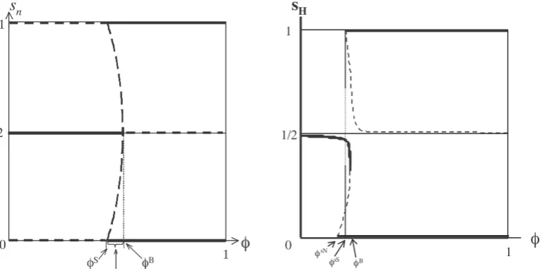
In the course of many years the conclusions of this theory were supported by the numerical simulations only. For this moment quite complete analytic study was carried out only for symmetric CP models. In this case the general picture describing stability of long-run equilibria is the following “tomahawk diagram”, see Figure 1, left-hand side. Here the measure of trade freenessϕ is, in some extent, inverse value to transportation costs, the bold lines contain all stable long-run equilibria, dashed “fork” is a set of all unstable equilibria. Along with “break point”ϕB _{mentioned above, the diagram contains so-called “sustain point”ϕ}S_{— the minimum level of freeness} making total agglomeration equilibria stable. Robert-Nicoud (2005) provides the first analytic proof of the CP model’s main features, namely that the break point comes before the sustain point (in terms of freenessϕ) and that it has at most three locally stable equilibria for any given level of openness. Mossay (2006) proved an existence and uniqueness of short-run equilibrium in symmetric CP model for all admissible values of parameters.

Studying of symmetric CP models allows to obtain very important conclusion: the resulting asymmetry (i.e. agglomeration) is a well-formed result even under condition of initial symmetry. In other words, agglomeration process may be interpreted in frameworks of “second nature”, i.e. as result of patterns human activity. Theorist can be interested, however: Are the trade and agglomeration pictures obtained robust against asymmetry or specific to symmetry?

To answer the appeal of the empirics, some numerical simulations show that certain qualitative conclusions can not survive in asymmetric case, e.g. relative positions of break pointsϕB _{and sustain pointsϕ}S _{(see for example,} Appendix C.1 to Chapter 2 of Baldwin et al. (2003), so called “broken tomahawk” on Figure 1, right-hand side). Moreover, Berliant and Kung (2009) show that symmetric case is singular in some sense.

Generally asymmetry remains weakly studied. The reason for lack of comprehensive analytic study of asym-metric CP model is substantial complexity of appearing problems, addressed in Baldwin et al. (2003, p. 53) pessimistically:

“Unfortunately, the intense intractability of the CP model means that numerical simulation of the model for specific values .... is the only way forward.”

Our contribution

The present paper aims to overcome this seeming “intractability” and give a complete study of Krugman’s CP model with and without initial heterogeneity, achieving the complete comparative statics of equilibria with respect to main exogenous parameters.

Note that there are two partial cases when result of struggle between agglomeration and dispersion forces is obvious. On perfectly competitive market dispersion forces prevail. Starrett’s impossibility theorem is one of impressive evidences of this idea. On the other hand, purely monopolistic competitive market is domain of agglomeration forces. More exactly, excluding of perfectly competitive agricultural sector from this model tends to existing of agglomerated equilibria only, i.e. resulting force for all market forces listed above in the case of monopolistic competition is agglomeration force. Thus Krugman’s CP model may be considered as mixed economymodel joining features of both perfectly competitive and monopolistic competitive markets. As a natural measure of relative weight of monopolistic-competitive sector an expenditure share of industral varieties may be taken. Moreover, intensity of agglomeration effects depends on elasticity of substitution, because its inverse is interpreted traditionally as “love for variety”. Note that this point of view is not brand new. For example, in Combes et al. (2008), pp.151-152, we read “Product differentiation plays a key role in the model... In other words, when varieties are homogeneous, dispersion is the only stable equilibrium. Conversely, when varieties are more differentiated, the likelihood of agglomeration is higher because the competition effect is weakened” and “Regarding the share of the manufactured good, it is readily verified that the values of τS _andτB _{increase with}

µ, and so does the probability that agglomeration occurs. This is because a larger share of the manufacturing sector, on which the snowball effect is built, makes the agglomeration force stronger.” Nevertheless, this idea was not supported by intensive analytical studiesand all conclusions concern symmetric case only. In our studies, prevailing or countervailing of agglomeration and dispersion forces is considered in terms of relative weights of perfectly competitive and monopolistic competitive sectors, which is measured mainly by expenditure shares.

share of industrial labor λ in home country. First we study relative industrial wage which is the fraction of industrial wage in home country to foreign wage. Propositions 1 and 3 show that:

(1) relative wageincreasesmonotonically with respect to home share of agricultural population;

(2) under sufficiently small transportation cost (very free trade) relative wage increases monotonically with respect to share of industrial labor;

(3) under sufficiently big transportation cost relative wagedecreaseswith respect to industrial labor share. Further we study industrial price indices in both countries and relative price index, which is home industrial price index divided by foreign one. Proposition 4 says that home industrial price index grows in home share

θ of agricultural population, whereas foreign price index decreases, so relative price index grows. Influence of industrial labor share growth is opposite — relative price index decreases with respect to industral labor share.

More important for further study of agglomeration is the study of relative welfare, i.e. utility value obtained by representative consumer in equilibrium. Proposition 5 says that relative welfare always increases in the agri-cultural share. Proposition 6 say that behavior of relative welfare in industrial labor share is more complicated and generally non-monotone. Under given parameters, including transportation cost and agricultural labor share, there can be zero, one, two or three interior values of industrial share yielding welfare equalization between the two countries (such point is a candidate for interior equilibrium when migration is allowed). No more than one of them is a candidate for a stable equilibrium. Under sufficiently small transportation costs for any fixed agricultural population our industral workers are always relatively better off when having more industrial compatriots. But under sufficiently big transportation costs for any fixed agricultural population there exist an optimal (for them) share.

Sections 4.1 and 4.2 study long-run equilibria describing migration: agglomerated and interior respectively. Obtained analytical results (as well as results of simulations) show that the general picture of agglomeration pro-cesses differs depending on degree of region’s asymmetry. Under small asymmetry the general picture of ag-glomeration patterns with respect to trade freeness is qualitatively similar to well-known one under symmetry “tomahawk” picture, it becomes just asymmetric. We provide the formal proof for this robustness of symmetric theory in the case of moderate asymmetry: any country can become the “core”. In contrast, under big asymmetry the pattern is qualitatively different: only agriculturally big country can become the core in agglomeration process, but the smaller one is doomed to be a periphery. We find the threshold or lower bound on asymmetry (in terns of other parameters) when only one core is predetermined by “first nature.” Below this bound ambiguity remains, but the higher is asymmetry, the more “probable” is agglomeration in the direction of the bigger country. Something like this was previously shown in simulations, see Baldwin et. al (2003). Now we combine known symmetric theory and known asymmetric simulations into general theoretical picture.

As to interior long-run equilibria, in section 4.2 we obtain comprehensive analytical results on their existence, number and stability under given parameters, generalizing results from Robert-Nicoud (2005) and giving more direct and intuitive proof.

To further motivate our interest in asymmetry of immobile (or, “agricultural”) populations, note that it may be considered (ceteris paribus) as equivalent to the market potentialdifferences. There is a series of empirical evidences showing that this asymmetry causes unavoidable differences across regions in wages (nominal and real), cost-of-living’s levels (or price indices) etc, see, for example, Cecchetti et al (2002), Hanson (2006), Roos (2006), Beenstock and Felsenstein (2008), Klaesson and Larsson (2009).

not robust. Generically, this class of bifurcations is a myth, an urban legend.” We agree that bifurcation itself goes away, but more important is that qualitative features and patterns of agglomeration still remain.

2

Core-Periphery Model

This paper studies the classical Krugman’s CP model, only with asymmetry of the two trading regions or countries: “Home”Hand “Foreign”F. The manufacturing sector in both countries is a standard Dixit-Stiglitz monopolistic competition industry with specialized labor that produces varieties or brands of “industrial good”. Each manu-facturing firm employs the labor of industrial workers and produces a single variety subject to increasing returns. Namely, production of varietyirequires a variable input involvingmunits of industrial-worker labor per unit of output produced and a fixed input of f units of this labor. In symbols, the cost function isC(i) = (f+m·x(i))·w, wherexis a firm’s output andwis the industrial workers’ wage. Note that wagewmay differ across regions, while fixed f and marginal variablemcosts are the same for bothH andF. In contrast, the agricultural sector produces a homogeneous good under perfect competition and constant returns using only the labor of agricultural workers. We normalize the model assuming that agricultural production takesma=1 unit of agricultural labor to make one unit of the homogeneous good and agricultural fixed costs fa=0.

The total amount of industrial labor denoted byL>0 andLa>0 denotes total amount of agricultural labor. Theshareof industral labor resided in home regionH is a numberλ ∈[0,1], analogously,θ∈(0,1)the relative share of agricultural population in regionH. It implies that supplies of industral and agricultural labor in region HareλLandθLarespectively. Analogously, labor supplies in regionF are(1−λ)Land(1−θ)La. In the short-run equilibrium concept is supposed that the values of shares λ andθ are fixed. Without loss of generality we shall assume thatθ>1/2, i.e. agricultural population of home region is greater or equal to foreign agricultural population. Perfectly competitive agricultural sector technology is uniform for both regions, the only difference concerns the numbers of laborers. Transportation of agricultural good assumed costless, thus prices for both countries are equal, which implies equalization of wage rateswaacross regions. Agricultural marginal costma=1, consequentlywa=1.

The goods of both sectors are traded between countries, and trade in industral sector trade incur iceberg-type trade costs, whereas trade in agricultural sector goods is frictionless. Specifically, it is costless to ship industrial goods to local consumers but to sell one unit in another region, an industrial firm must produce and shipτ >1 units. The idea is thatτ−1 units of the good “melt” in transit like an iceberg melts driving across an ocean. As usual,τ captures all the costs of selling to distant markets, including transport costs and tariffs, τ−1 being the tariff-equivalent of these costs.

The typical consumer in each region has a two-tier utility function. The upper tier determines the consumer’s allocation of expenditure between the homogeneous agricultural good, and the differentiated sector. The second tier dictates the consumer’s preferences over the various differentiated industrial varieties and the choice within this sector. The specific functional form of the upper tier is Cobb-Douglas that makes the sectoral expenditure shares constant (under CES at the lower tier). In symbols, preferences of a typical consumers are described by utility function:

U=Mµ·Q1−µ, 0<µ<1 (1) whereQis the consumption of the homogeneous good andMis the composite consumption utility of all differenti-ated varieties of industrial goods. Traditionally the functional form of the lower tier is represented by CES-function (constant elasticity of substitution) functionM=

_N

∑

i=1

qρ_i

1_ρ

for discrete varieties orM=

_N

´ 0

q(i)ρdi

ρ1

contin-uous case1. Here 0<ρ<1 is a parameter related to the elasticity of substitution 1<σ<∞as followsρ=σ−1

σ .

NumberNcharacterizes assortment of varieties or number of firms producing these varieties.

Each consumer (being of industrial or agricultural type) owns a unit of labor supplied inelastically to the market in exchange of both types of goods produced in both countries, so the industrial consumer’s problem is

U(Mm,Qm)→max s.t.

ˆ NH 0

pHH(i)qm_HH(i)di+

ˆ NF 0

pFH(j)qm_FH(j)dj+1·Qm=wH

and the agricultural worker finds

U(Ma,Qa)→max s.t.

ˆ NH 0

pHH(i)qaHH(i)di+

ˆ NF 0

pFH(i)qaFH(i)di+1·Qa=1,

whereqm_HH(i)denotes the industrial worker’s consumption ofi-th variety produced and consumed in home region, whereasqm_FH(j)denotes her consumption of j-th variety imported from foreign country. ValuespHH(i)andpFH(j) are the corresponding prices. Recall that price of homogeneous agricultural good is normalized to 1. ValuesNH andNF denote the numbers of firms in regionsH andF respectively. Similar notations are used for consumer’s problem of agricultural workers, and for consumers in another country. Now the home aggregate demand for agriculture good isQ=λL·Qm+θLa·Qa, aggregate demands for each varietyqHH(i) =λLqmHH(i) +θLaqaHH(i), qHF(i) = (1−λ)Lqm_HF(i) + (1−θ)Laqa_HF(i), etc.

It is well known under CES-function the analytical form of aggregate demand in countryHfor home produced i-th variety is equal to

qHH(i) =

(wH·λL+θLa)·µ·p−_HHσ(i)

´NH 0 p

1−σ

HH (j)dj+

´NF 0 p

1−σ

FH (j)dj

. (2)

In turn, aggregate demand in foreign region fori-th variety produced inHis equal to

qHF(i) =

(wF·(1−λ)L+ (1−θ)La)·µ·p−HFσ(i)

´NH 0 p

1−σ

HF (j)dj+

´NF 0 p

1−σ

FF (j)dj

. (3)

Home demand for foreign produced goodqFH(j)and foreign demand for foreign produced goodqFF(j), j∈[0,NF]may be obtained analogously.

Each home producer maximizes her profit

πH(i) =qHH(i)·(pHH(i)−wHm) +qHF(i)·(pHF(i)−wH·τ·m)−wH·f,

whereqHH(i),qHF(i)are defined in (2) and (3), correctly anticipating the demand for his/her variety and perceiving the competitors’ variables fixed, because everyone is “small enough”. Note that production costs m are also uniform for both regions. Maximizing this profit with respect topHH(i)andpHF(i)we obtain the following values of prices

pHH(i)≡pHH=

wH·m·σ

σ−1 , pHF(i)≡pHF=

wH·τ·m·σ

σ−1 , (4)

which are uniform for all product varietiesi∈[0,N]. Analogously,

pFH(j)≡pFH=

wF·m·τ·σ

σ−1 , pFF(j)≡pFF=

wF·m·σ

σ−1 (5)

1_{The limitations of Cobb-Douglas+CES modeling is that it is too specific to obtain more interesting comparative statics: it shows too}

The concept of short-run equilibrium implies that share λ is fixed (as well as θ), whereas the free-entry condition states that positiveness of profit in industry causes increasing of number of firms until profit becomes zero. For example, for home producers this Zero-Profit ConditionπH(i) =0, taking into account formulas (2)-(5), is of the following form

(wHλL+θLa)µp_HH−σ·(pHH−wH·m) NH·p1_HH−σ+NF·p1_FH−σ

+(wF(1−λ)L+ (1−θ)La)µp

−σ

HF·(pHF−wH·τ·m) NH·p1_HF−σ+NF·p1_FF−σ

=wHf.

Let’s substitute for thispHH−wHm=

wH·m·σ

σ−1 −wH·m=

wH·m

σ−1 andpHF−wH·τ·m=

wH·τ·m

σ−1 into previous equation. We obtain

(wH·λL+θLa)·µ·p−HHσ NH·p1HH−σ+NF·p1FH−σ

+τ·(wF·(1−λ)L+ (1−θ)La)·µ·p

−σ

HF NH·p1HF−σ+NF·p1FF−σ

=(σ−1)f

m .

The left-hand expression is equal to total output of home-produced variety covering the total demand. This pro-duction requires the following amount of industrial labor

f+m(σ−1)f

m = f·σ.

Consequently the total industrial labor demand is equal toNH·f·σ and from labor market equilibrium condition we obtain that the mass of home firms

NH=

λL

f·σ,

analogously

NF=

(1−λ)L f·σ .

Substituting expressions for prices (4), (5) and just obtained NH, NF into Zero-Profit equation we obtain, after simplifying, the following equation:

µ λwH+θ·

La

L

λw1_H−σ+ (1−λ)ϕ·wF1−σ

+ϕ (1−λ)wF+ (1−θ) La

L

λ ϕwH1−σ+ (1−λ)w1_F−σ

!

=wσ_H, (6)

whereϕ=τ1−σ _{∈(0,1)may be interpreted as a measure of trade “freeness” or “openness”. Taking into account}

normalization of agricultural parameters (i.e. marginal costs wage rate are supposed to be equal to 1), a commodity balance of agricultural product may be written as

(1−µ) (wH·λL+wF·(1−θ)L+1·La) =La

or

λwH+ (1−λ)wF =

µ

1−µ·

La

L (7)

where La, L are the total amounts of agricultural and industrial labor in the world, wH and wF are industrial wages, home and foreign respectively,µ characterizes expenditure share of industrial production andλ is a share of industrial labor in home region.

In contrast, the concept oflong-run equilibriumimplies that there can be a location choice. Agricultural labor-ers still assumed to be immobile, but share of industrial worklabor-ersλcan change due to migration between the regions. Let’s fix an arbitraryλ ∈(0,1) and calculate allshort-runequilibrium values of pricespHH,pHF,pFH,pFF, de-mandsqm_HH,qm_HFqm_FHqm_FF, and numbers of firmsNH,NF (see (4), (5)). To obtain the demand ofindustrialworkers only, it is sufficient to putLa=0 in (2) and (3). Then substitute the obtained equilibrium values of industrial labor demand (for both countries) into utility function (1), as result we get theindustrial welfares VH(λ)andVF(λ)for Home and Foreign countries at the value of shareλ∈(0,1)(for rather explicit formula of welfare see subsection 3.4). An inequalityVH(λ)>VF(λ) is considered in long runas incentive to migration from Foreign to Home country and vice versa. One of the popular migration dynamics is so-calledad hocmigration equation:

˙

λ=λ(VH(λ)−(λVH(λ) + (1−λ)VF(λ))) =λ(1−λ) (VH(λ)−VF(λ))

In thelong-run equilibriumthe market and agglomeration determine the equilibrium valueλ0_{of share of industrial}

labor in our country, such that no migration occurs: ˙λ =0. The equilibria can be “agglomerated” that means eitherλ0_{=0 orλ}0_{=1, i.e. one country becomes pure agricultural one. Alternatively, a “interior equilibrium”}

implies both countries producing manufacturing goods and the equal real wages for both regionsVH(λ0_{) =V}

F(λ0), 0<λ0_<1.

We are going to analyze the asymmetric CP model in two stages. First we derive solutions and their com-parative statics for short-run equilibria, interpreted as equilibrium in international trade, and having independent value itself. Then, using these results we completely describe the long-run equilibria, i.e., the resulting agglomer-ation/dispersion outcomes.

3

Short-run Equilibria

3.1 Equilibrium equations and existence

We get the following two equations (see equations (6), (7) above) connecting nominal wages with exogenous parameters

µ λwH+θ·

La

L

λw1_H−σ+ (1−λ)ϕ·wF1−σ

+ϕ (1−λ)wF+ (1−θ) La

L

λ ϕwH1−σ+ (1−λ)w1F−σ

!

=wσ_H,

La L =

1−µ

µ ·(λwH+ (1−λ)wF),

whereϕ=τ1−σ _{is “trade freeness” andw}

HandwF are wages of industrial labor in Home and Foreign countries respectively.

Substituting second equation into the first one we derive the following simpler one with respect to relative wage wH

wF:

(1−λ)h1−((1−θ) +µθ)(1−ϕ2_)−ϕ·wH

wF

σi

−

−λ

1−((1−µ)θ+µ) 1−ϕ2_wH

wF −ϕ·

wH

wF

1−σ

=0

(8)

Solution of this equation allows to obtainnominalwages from the following equation, which is equivalent to (7)

wH=

µ

1−µ ·

La·w_wH_F L

λwH

wF + (1−λ)

Based on the simplification obtained, the following result generalizes existence and uniqueness of short-run equilibrium (see Mossay, 2006) to the asymmetric case.

Proposition 1. i) There exists a unique positive value of Relative Nominal Wage wH

wF defined by equation(8).

ii) This value satisfies the following inequalitiesϕσ1 <wH

wF <ϕ

−1

σ. In the case of “costless trade”,ϕ=1, an

identity wH≡wF holds (“integrated equilibrium”). For analytical proof see Lemma 1 in Appendix A.

From equations (8) one can see that relative wage depends on shares θ,λ only but not on absolute values of industrial and agricultural labors (LandLa). Similarly, based on (9), the wage itself depends on fraction of industrial labor to agricultural one La

L but not on the absolute size of global labor. Note that this is a natural consequence of the linear homogeneity of preferences. Costs do not affect wages.

3.2 Changes in wages

From equation (8), the relative wage is an implicit function of labor sharesθandλ, as well as trade freenessϕand utility function parametersµ andσ. We start deriving the comparative statics of equilibria with respect to labor shares.

Denotex=wH

wF for short, then equation (8) takes the following form

(1−λ)(1−((1−θ) +µθ)(1−ϕ2)−ϕ·xσ)−λ(1−((1−µ)θ+µ)(1−ϕ2))x−ϕx1−σ) =0.

An implicit functionx(λ,θ,µ,ϕ,σ)is solution to this equation. Immediately one can derive two special cases. Underϕ=0 transportation costs are infinitely large, trade is impossible and thisautarkyyields wH

wF =

(1−λ)θ

(1−θ)λ

which increases with respect toθ, decreases with respect toλ and remains unaffected by other parameters. Under

ϕ=1 trade is costless and so-calledintegrated equilibriumyields wage equalization wH

wF ≡1 independently of any

parameters. The equalization was known under symmetry of labor, but now we see that it is a general fact. Now consider the most interesting case 0<ϕ<1 of non-trivial trade cost. Applying the implicit function theorem to previous equation we obtain the following

Proposition 2. (Comparative statics with respect to agricultural labor share)

i) Nominal wage in Home country wH increases while foreign wage wF decreases with respect to Home agri-cultural population shareθ, thereby relative industrial wage wH

wF also increases.

ii) Home nominal wage is greater than foreign wage (wH >wF) iff the share of home agricultural labor is sufficiently large, namelyθ>λ+ (1−2λ)ϕ

(1+ϕ)(1−µ). The opposite strict inequality implies reverse wage relation.

iii) Under sufficiently big asymmetry of industrial labor, namelyλ+ (1−2λ)ϕ

(1+ϕ)(1−µ) >1or

λ+ (1−2λ)ϕ

(1+ϕ)(1−µ) <0there is no wage equalization for any sharesθ∈(0,1). For analytical proofs see Lemmas 1, 2 and 3 in Appendix A.

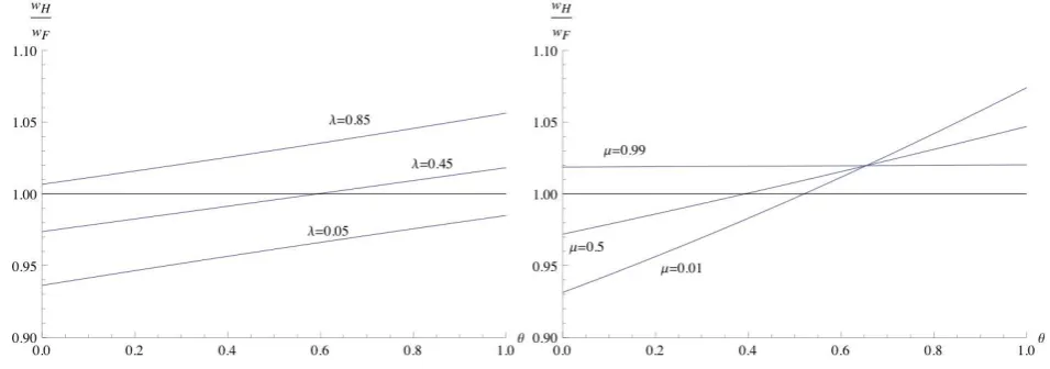
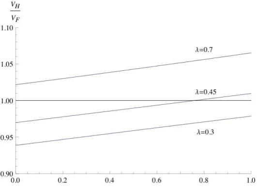
Figure 2: Left-hand plot: Relative wages with respect toθforµ=0.7,ρ=0.75,ϕ=0.75 and three values ofλ. Right-hand plot: Relative wages with respect toθ forλ=0.65,ρ=0.75,ϕ=0.75 and three values ofµ.

θ0_{≈0.6. Also we plot relative wage three values of expenditure share –µ=0.01 (close to perfect competition),}

intermediateµ =0.5 andµ =0.99 (close to monopolistic competition).

To interpret the monotonic increase, take into account that agricultural shareθindirectly reflects the size of the market for industrial goods. Bigger market requires more industrial labor whose supply is fixed in the short-run. Note also there is no difference in tendencies for perfectly competitive and monopolistic competitive sectors of economy. It should be mentioned only that for “almost monopolistic competitive” economies (µ ≈1) relative wage is (almost) neutral to agricultural labor allocationθ because of its negligibility. On the other hand, in the case when economy close to perfect competition (µ≈0) its monopolistic competitive sector is more sensitive to home market size. As to realism of monotonicity conclusion, there is empirical evidence that market size really positively affects wages and that the industrial structure matters, see, for example, discussion in Klaesson and Larsson (2009).

Considering dependence of wages onλ we find that in this case answer is ambiguous and heavily depends on agricultural heterogeneity indexdefined as followsα =2θ−1=θ−(1−θ)(we assume thatθ >1/2). It measures degree ofasymmetryin the agricultural labor distribution,α=0 for symmetric model andα=1 in the case of total asymmetry forθ=1. Define the following value

ϕw(µ,α) =

v u u u t

1−α2

1+µ

1−µ

2

−α2

∈(0,1)

which increases with respect to asymmetryα and decreases w.r.t. expenditure shareµ.

Proposition 3. (Comparative statics with respect to industrial labor share)

When “freeness” exceeds the threshold:ϕ>ϕw_{(µ,α), then relative industrial wage} wH

wF increases with respect to

industrial labor shareλbut decreases under smaller “freeness”ϕ<ϕw_{(µ,α). In the caseϕ=ϕ}w_{(µ,α)relative} wage wH

wF does not depend onλ.

For analytical proof see Lemma 4 in Appendix A.

Figure 3: Left-hand plot: Relative wages with respect toλ forθ=0.65,ρ=0.75,ϕ=0.5 and three values ofµ. Right-hand plot: Threshold values of expenditure share µw_{with respect to asymmetry measure α =2θ−1 for} three values ofϕ.

Corollary 1. Relative wage wH

wF increases with respect to industrial labor shareλ in the case

µ >µw_{(ϕ,α), decreases whenµ <µ}w_{(ϕ,α)and does not depend onλ forµ =µ}w_(ϕ,α)where

µw(ϕ,α) =

p

1−(1−ϕ2_)α2_−ϕ

p

1−(1−ϕ2_)α2_+ϕ.

This corollary allows more clear interpretation of struggle in the outcomes between agglomeration and disper-sion forces. On a near perfectly-competitive market (µ ≈0) dispersion forces prevail, and increasing the home industral labor shareλ (or, equivalently number of firmsNH=

λL

f·σ) negatively affects the relative wage

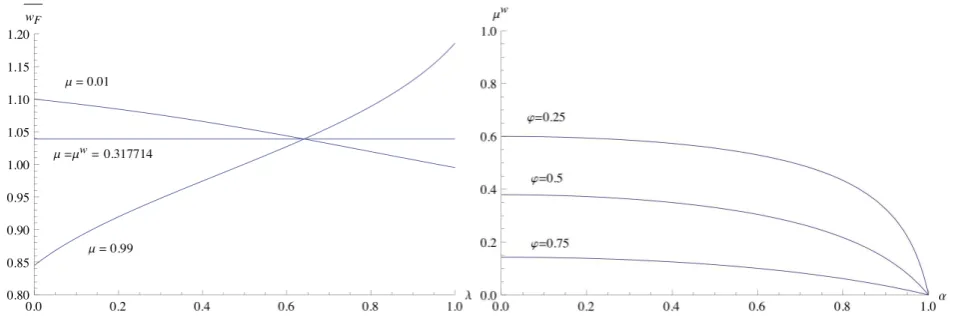
wH wF . On the other hand, on a monopolistic-competitive market (µ ≈1) domination of agglomeration forces tends to increase the relative wage with respect toλ. Increasing the expenditure shareµ of the monopolistic competitive sector weakens dispersion forces, while agglomeration forces are enhanced. At threshold valueµw_{, agglomeration} and dispersion forces compensate each other. On left-hand side of Figure 2 three outcomes of force’s struggle are represented: when expenditure shareµ =0.01 is small dispersion wins, when it is large µ =0.99 then ag-glomeration prevail and only forµ =µw_{≈0.317714 tie happens. The right-hand side illustrates dependence of} threshold value on asymmetry measure of agricultural labor allocationα=2θ−1∈(0,1)and trade “freeness”ϕ

for three values. Due to Corollary 1, an areaabovethe threshold curveµw_{(ϕ,α)covers the cases of increasing of} relative wage. We see that increasing of trade “freeness” makes this area wider, i.e. helps generate agglomeration. The same occurs under increasing of asymmetry in the agricultural population allocationα =2θ−1. The large concentration of agricultural population in home country attracts more industrial (i.e. agglomeration) forces and amplifies their impact.

3.3 Changes in Price Indices (or Agricultural Welfare)

Prices pi j defined in equations (4)-(5) allow to define the index of cost of living, somewhat vaguely called “price index”,PH for Home-Country andPF for foreign one. This index is the expenditure function at utility 1, i.e. the amount of money needed to maintain a unit level of gross utility under these prices. It is standard in CP model to express the index in both as

PH= λw1H−σ+ (1−λ)w1F−σϕ

₁₋1_σ

, PF = λ ϕwH1−σ+ (1−λ)wF1−σ

(see for detailsComparative Statics of Price Indicesin Appendix I).

Since agricultural workers always have unit income, the inverse price index directly measures their utility as Va₌wa

Pµ = 1

Pµ. The changes in both with respect to relative agricultural population are described as follows.

Proposition 4. i) Nominal price index for any region increases with respect to its own agricultural population

share, while foreign nominal price decreases, i.e., PHincreases inθwhereas PF decreases.

ii) Relative price indices PH/PF increases with respect to agricultural population shareθ, thereby relative welfare of agricultural workers Va

H/VFa= 1 (PH/PF)µ

becomes more favorable for the country with decreasingθ.

iii) Relative price indices PH/PF decreases with respect to industrial population share λ, thereby relative welfare of agricultural workers V_Ha/V_Fa= 1

(PH/PF)µ

becomes more favorable for the country with increasingλ.

iv) Price indices PHand PF (as well as agricultural welfares V_Haand V_Fa) are equalized under condition 1−((1−θ) +µθ)(1−ϕ)

1−((1−µ)θ+µ) (1−ϕ) =

λ

1−λ

_σσ₋₁

.

For all given θ,ϕ,µ,σ there exists λ ∈(0,1) satisfying this equation. On the other hand, for some values of

λ,ϕ,µ,σprice indices of two countries may be non-equalizible for allθ∈(0,1). v) Price index inequality PH>PF holds if and only if

θ> (1−µ) +µϕ

(1−µ)(1−ϕ)−

(1−µ) + (1+µ)ϕ

(1−µ)(1−ϕ)

1+₁₋λ_λ

σ σ−1

or, equivalently,

λ

1−λ <

1−((1−θ) +µθ)(1−ϕ) 1−((1−µ)θ+µ) (1−ϕ)

ρ

.

For analytical proof see Lemmas 5, 6 and 7 in Appendix A.

Note that left-hand side of equalization condition ₁1−₋((₍₍₁1₋−θ)+µθ)(_µ)θ+µ)(1₁−₋ϕ)_ϕ) under variation of θ ∈(0,1) takes the values in limited interval between _{(1−µ)+µϕ}ϕ and (1−µ)+µϕ_ϕ , whereas the right-hand side changes in unlimited interval, i.e,

λ

1−λ

_σσ₋₁

∈(0,∞) for various λ ∈(0,1). Thereby, there always exist some shares of industrial laborλ that equalize price indices and welfares of agricultural workers, but changes in agricultural labor may be insufficient for this task under givenθ∈(0,1)and other parameters.In other words, migration of industrial labor producing varieties matters more for agricultural welfares equalization than changes in agricultural labor, even if

concede possibility of the agricultural migration.

At Figure 4 the proposition and all three (equalizible and non-equalizible) situations are represented. We see that under sufficient asymmetry in industrial labor, price indices need not equalize between countries, it means Law of one price fails. We can compare our two propositions with traditional international trade and factor-price equalization in Hecksher-Ohlin model with specific factors used in two industries. Like there, factor endowments of the countries matter in our model and differences in wages or prices depend on parameters in natural direction: a factor in shorter supply becomes more expensive.

Figure 4: Changes in relative price index with respect to asymmetry inθ for µ =0.7,ρ =0.75, ϕ=0.75 and three values ofλ.

3.4 Changes in industrial welfares

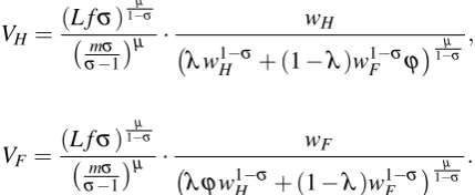
The industrial welfare in a country is defined by dividing industrial nominal wage wby the price index P. For Home country it equals to

VH=

(L fσ)1−µσ

mσ σ−1

µ ·

wH

λw1_H−σ+ (1−λ)w_F1−σϕ₁₋µ_σ ,

and for Foreign it is

VF=

(L fσ)1−µσ

mσ σ−1

µ ·

wF

λ ϕw1_H−σ+ (1−λ)w1_F−σ

µ 1−σ

.

Thus relative welfare may be expressed in terms of relative wage as follows

VH VF

=wH wF

  

λ+ (1−λ)ϕwH

wF

σ−1

λ ϕ+ (1−λ)wH

wF

σ−1   

µ σ−1

. (10)

Next proposition extends the comparative statics of previous two propositions onto real wages (utilities) of indus-trial labor in two countries.

Proposition 5. i) Relative industrial real wage VH

VF as well as home welfare VH of industrial labor increase with

respect to home agricultural population shareθ.

ii) There exist values ofλ,ϕ,µ,σwhen industrial welfares of two countries are non-equalizible, i.e., VH6=VF for allθ∈(0,1).

For analytical proof see Lemma 5 in Appendix A.

Figure 5: Comparative statics of relative welfare with respect toθforµ=0.7,ρ=0.75,ϕ=0.75 and three values ofλ.

Interpreting the monotonicity observed, we can say that in this case there is no conflicts between perfect competitive and monopolistic competitive sectors. Indeed, in the case µ =0 we obtain from (10) that relative welfare is similar to relative wage wH

wF

that is increasing function with respect to agricultural labor share θ. To approximate monopolistic competitive case µ =1 we use equivalent representation of relative welfare (see for detailsComparative Statics of Industrial Welfaresin Appendix A)

VH VF

=

xρµ (1−µ)θ−((1−µ)θ+µ)ϕx

(1−µ)(1−θ)x−((1−θ) +µθ)ϕ

_σµ₋₁

,

wherex=

wH wF

σ

. Then forµ =1 we obtain that relative welfare is similar to positive power of relative wage

wH wF

2σ_σ−−₁1

that is increasing function with respect to agricultural labor shareθ.

Comparative statics with respect to industrial labor share λ is more sophisticated. Traditionally general case is divided into two sub-cases. The first one is so calledBlack Hole,characterized by inequalityρ=σ−1

σ 6µ,

or equivalently, 1

σ =1−ρ >1−µ with the following interpretation — love for industrial variety exceeds the

expenditure share for agricultural good. The opposite case characterized by No-Black-Hole Conditionρ >µ

will be considered as main one. In this case one can define the following critical point

ϕB(ρ,µ,α) =ρ−µ

ρ+µ

v u u u u t

1−α2

1+µ

1−µ

2

−α2

whereα=2θ−1, coinciding in symmetric caseα =0 with break-pointϕB_{mentioned in Introduction.}

Proposition 6. i) Let Black-Hole Condition ρ 6µ holds. Then relative welfare VH VF

increases with respect

to industrial labor share λ. There exists the unique value λ0_{∈(0,1) yielding industrial welfare equalization}

VH(λ0) =VF(λ0).

ii) Assume No-Black-Hole Conditionρ >µ holds andϕ>ϕB(ρ,µ,α). Then relative welfare VH VF

increases

with respect to industrial labor shareλ and there is at most one value λ0_{∈(0,1)yielding welfare equalization}

iii) Assume No-Black-Hole Conditionρ>µ holds andϕ<ϕB_{(ρ,µ,α). Then relative welfare}VH VF

increases

with respect to industrial labor shareλfor sufficiently smallλ>0and derivative ∂

∂ λ

VH VF

changes its sign not more

than twice for allλ ∈(0,1). Therefore there is at most one three valuesλ ∈(0,1) yielding welfare equalization VH(λ) =VF(λ).

For analytical proof see Lemmas 9, 10 in Appendix A.

We obtain this threshold effect in terms of trade freenessϕ. Proposition 6 may be equivalently reformulated in terms of threshold value of expenditure share µ, though there is no the corresponding explicit form of this threshold.

Corollary 2. For all(ρ,α,ϕ)∈(0,1)3_{there is defined a continuous functionµ}B_{(ρ,α,ϕ)satisfying the following} conditions:

i) function values0<µB_{(ρ,α,ϕ)<ρ, moreoverµ}B_{(ρ,α,ϕ)decreases with respect toϕandα} ii) For all µ >µB_{(ρ,α,ϕ) relative welfare} VH

VF

increases with respect to industrial labor shareλ and there

exists not more than one valueλ0_{∈(0,1)yielding welfare equalization VH(λ}0_{) =V}

F(λ0) iii) Forµ <µB_{(ρ,α,ϕ)relative welfare}VH

VF

increases with respect to industrial labor shareλ for sufficiently

smallλ >0and derivative ∂

∂ λ

VH VF

changes its sign not more than twice for allλ ∈(0,1). Therefore there exists not more than three valuesλ ∈(0,1)yielding industrial welfare equalization VH(λ) =VF(λ).

Indeed, the threshold functionµB_{(ρ,α,ϕ)may be obtained as implicit function defined by equation}

F(ϕ,ρ,µ,α) =ϕ−ρ−µ

ρ+µ

v u u u u t

1−α2

1+µ

1−µ

2

−α2

=0.

It is obvious thatF(ϕ,ρ,µ,α)strictly increases with respect toµ, i.e. ∂F

∂ µ >0 for all admissible arguments, thus

by the Implicit Function Theorem there exists differentiable functionµB_{(ρ,α,ϕ)and}

∂ µ

∂ α =−

∂F

∂ α

∂F

∂ µ

<0,

∂ µ

∂ ϕ =−

∂F

∂ ϕ

∂F

∂ µ

<0

becauseF(ϕ,ρ,µ,α)obviously increases with respect toα andϕ. We need not consider Black-Hole case sepa-rately, sinceµ >ρimplies µ>µB_{(ρ,α,ϕ). In other words,Black Hole is simply a partial case of monopolistic} competition’s prevailing.

Note that equalization valuesVH(λ0_{) =V}

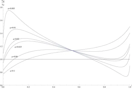
F(λ0) are exactly interior long run equilibrium values of industrial labor shares. More detailed consideration of interior long run equilibria is postponed until section 4.2. Claims (ii), (iii) with No-Black-Hole Condition are illustrated in Figure 6. When “freeness”ϕ increases gradually from 0.003, to 0.1, the sinus-shape curve of relative welfareVH

VF

(λ)becomes less and less steep in the middle, arriving finally at monotone increasing shape. The curve changes as a piece of wire, whose left end is pulled down but right end up (seemingly, all curves turn around one point, but it is an illusion). In the beginning, under 0.003, the curve intersects the horizontal lineVH

VF

Figure 6: Different patterns of relative welfare forθ=0.55,µ=0.2,ρ=0.25 and various values of freenessϕ.

supplemented by thethird equilibrium(unstable one) after the left end of the curve hits 1 (say, under ϕ=0.02), but after biggerϕ=0.01 the middle and the rightmost equilibria disappear together, only one unstable intersection is possible. Similar picture—one intersection from below—remains true under further increase ofϕ>0.01, and remains also under Black-Hole Condition discussed in claim (ii), for allϕ. Note that increasing of relative welfare VH

VF

reflects predominance of agglomeration forces with directiontoward home country, while decreasing reflects the opposite process. Figure 6 demonstrates also that increasing of trade freeness supports agglomeration forces.

Further, Figure 7 illustrates how strengthening of monopolistic competition (i.e. increasing of expenditure share µ) changes correlation of agglomeration and dispersion forces. For small values of µ dispersion forces prevail and relative welfare decreases forming stable interior long run equilibria (see for details section 4.2). For sufficiently large values of µ outcome is opposite — relative welfare increases with respect to home industrial labor share. As for intermediate values — for example,µ=0.55 — dynamics of relative welfare may change not more then twice.

Possible absence of interior utility equalization under sufficiently big agricultural asymmetry occurring under

Figure 7: Different patterns of relative welfare forθ=0.6,ϕ=0.005,ρ=0.75 and various values of expenditure shareλ.

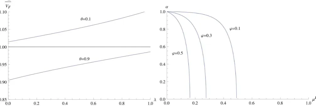
Figure 8: Left-hand plot: Absent utility equalization under big agricultural asymmetry:θ=0.9,µ=0.25,ϕ=0.7,

ρ=0.75.

Right-hand plot: Threshold values of expenditure share µB _{with respect to asymmetry measure α =2θ−1 for} three values ofϕ.

4

Asymmetry in Long Run

4.1 Agglomerated Long-Run Equilibria

The most popular migration dynamics model is so calledad hocdynamics for industrial labor shareλ

˙

λ =M(λ) =λ(1−λ) (VH(λ)−VF(λ)).

From this point of view there are two agglomerated long-run equilibria λ0_{=0 and λ}0_{=1 which are steady}

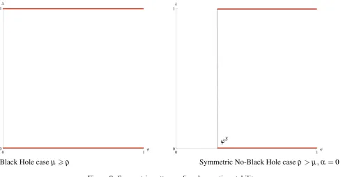
Black Hole caseµ>ρ Symmetric No-Black Hole caseρ>µ,α=0 Figure 9: Symmetric patterns of agglomeration stability

∂M

∂ λ (0)<0 and

∂M

∂ λ(1)<0 which is equivalent to inequalities

VH VF

(0)<1 and VH VF

(1)>1, respectively. Note that these inequalities may be well interpreted without any differential equations, the first inequality means that all industrial workers left Home country and none want to return, the second one means that all gathered in Home country and none want to leave.

In symmetric caseθ=1/2 one can obtain one of two typical pictures of stability depending on transportation costsτ>1 or, which is equivalent, on trade freenessϕ=τ1−σ _{∈(0,1]. The first one is so called “Black Hole”}

when both agglomerated equilibria are stable for all values ofϕ∈(0,1]and it appears in the caseρ=σ−1

σ 6µ.

Under “No Black Hole Condition” ρ>µ there exists “sustain point”ϕS _{∈(0,1) such that both agglomerated} equilibria are unstable for allϕ∈(0,ϕS_{)and they are both stable for allϕ∈(ϕ}S_,1].

Here the bold lines are sets ofstableagglomerated long run equilibria for various values of trade freenessϕ. Asymmetry in agricultural population brings two new cases. Without loss of generality we assume thatθ>1/2.

Proposition 7. i) Let Black-Hole conditionρ6µ holds. Then both agglomerated equilibriaλ=0andλ =1are stable for all values ofϕ,θ.

ii) Let No-Black-Hole condition ρ>µ holds andµ > ρ

1+2ρ. Then there exist0<ϕ

S

1 6ϕ0S<1such that

agglomerated equilibriumλ=0is stable if and only ifϕ>ϕS

0 andλ=1is stable if and only ifϕ>ϕ1S. Moreover,

ϕS

0 =ϕ1Sif and only ifθ =1/2. Sustain pointϕ0Sstrictly increases with respect toθ whileϕ1Sstrictly decreases.

iii) Let No-Black-Hole condition ρ>µ holds andµ < ρ

1+2ρ. Then there exist0<ϕ

S

1 6ϕ0S61such that

agglomerated equilibriumλ=0is stable if and only ifϕ>ϕS

0 andλ=1is stable if and only ifϕ>ϕ1S. Moreover,

ϕS

0 =ϕ1Sif and only ifθ=1/2,ϕ0S<1for allθ<

ρ+µ

2(1−µ)ρ andϕ

S

0 ≡1for allθ>

ρ+µ

2(1−µ)ρ. Sustain point ϕS

0 strictly increases with respect toθfor allθ∈

1 2,

ρ+µ

2(1−µ)ρ

whileϕS

1 strictly decreases for allθ.

For technical details see Lemmas 12, 13 in Appendix B.

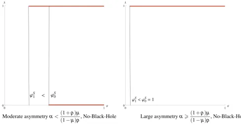
Moderate asymmetryα<(1+ρ)µ

(1−µ)ρ, No-Black-Hole Large asymmetryα>

(1+ρ)µ

(1−µ)ρ, No-Black-Hole

Figure 10: Asymmetric patterns of agglomeration stability

Sub-case ii) is analogous to its symmetric case except that each agglomerated equilibrium has specified sus-tain pointϕS

0 forλ =0 andϕ1S forλ =1. Finally, sub-case iii) when one of sustain points disappears is specific

to “sufficiently large” asymmetry in agricultural labor allocation. It is obvious that increasing of trade freeness supports agglomerationin both directions, while asymmetry in agricultural population is favorable for agglomer-ation in big country only. For sufficiently large measure of monopolistic competitionµ> ρ

1+2ρ thegeneral(i.e.

non-directed) agglomeration has some influence and ambiguity in agglomeration directions still remains, though asymmetry makes one of directions “more probable”. In opposite case, when monopolistic competitive sector is sufficiently weak, i.e.µ< ρ

1+2ρ directed agglomeration prevails and for sufficiently large asymmetry ambiguity

disappears.

Note additionally that for any givenρ>µ andθ sustain pointsϕS

0,ϕ1Smay be found as thesmallestroots of

equations

G(ϕ) =θ(1−µ)ϕµρ−ρ_{+ (1−θ(1−µ))ϕ} µ+ρ

ρ _=1,

H(ϕ) = (1−θ)(1−µ)ϕµ−ρρ _{+ (1−(1−θ)(1−µ))ϕ} µ+ρ

ρ _=1,

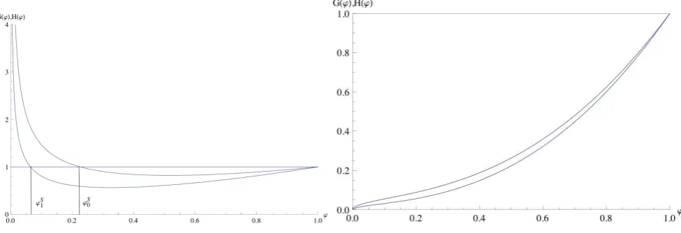
respectively (see proof of Lemma 13 in Appendix B). On the Figure 11 functions G(ϕ), H(ϕ) are plotted for No-Black-Hole (left-hand side) and Black-Hole (right-hand side) cases. Note thatϕ =1 is trivial root of both equations and sometimes (namely, for allθ> ρ+µ

2(1−µ)ρ) it is a smallest one. In other casesϕ

S

0,ϕ1S∈(0,1). In

No-Black-Hole caseρ >µ for allϕ ∈(0,1)inequalities ϕµ+ρρ _<1<ϕ µ−ρ

ρ _{hold, while left-hand sides of these}

equations are the weighted sums of termsϕµ−ρρ _andϕµ+ρρ_{. It is obvious that increasing in agricultural labor share}

θ, or equivalently in corresponding weight coefficient, pulls plot ofG(ϕ)up, while plot ofH(ϕ)goes down. Thus sustain pointsϕS

0, ϕ1S shift to the right and left, correspondingly. In Black-Hole case changes in θ do not have

Figure 11: Sustain points: No-Black-Hole and Black-Hole cases

4.2 Interior Long-run Equilibria

Interior long-run equilibria may be defined as interior steady statesλ0_{∈(0,1)of the samead hocdynamic equation}

˙

λ =M(λ) =λ(1−λ) (VH(λ)−VF(λ)).

which implies the equality of industrial real wages in both regionsVH(λ0_{) =V}

F(λ0). Stability conditions for this type of dynamics may be standardly expressed as∂M

∂ λ(λ

0_{)<0 which is equivalent to inequalities} ∂

∂ λ

VH VF

(λ0_)<0.

Note that these inequalities may be also interpreted without any differential equations. It means that the further immigration in Home country causes deceasing of relative welfare and leads to backward migration.

Recall the definition of break point

ϕB=ρ−µ

ρ+µ

v u u t

1−(2θ−1)2

1+µ

1−µ

2

−(2θ−1)2

Proposition 8. i) Let Black-Hole Condition ρ 6µ hold. Then there is at most one single interior long run equilibrium and ,in case of existence, it is always unstable.

ii) Let No-Black-Hole Conditionρ>µ holds andϕ>ϕB. Then there is at most one interior long-run equi-librium and ,in case of existence, it is always unstable.

iii) Let No-Black-Hole Conditionρ >µ holds and0<ϕ<ϕB_{. Then there is at most three interior long-run} equilibria.

Numerical simulation show that for appropriate values of the parameters, each of the cases in “not more than n” is possible, i.e. for ϕ >ϕB _{there are examples of exactly one or without any interior equilibrium, and for}

Pattern 0: No Break-Point, Sustain PointsϕS

0 =ϕ1S=0

Figure 12: Black Hole map:µ =0.5>ρ=0.25,θ=0.6

These patterns are represented by simulation results for specified values of ρ,µ,θ and for all values of in-dustrial labor shareλ and trade freenessϕ. Dark area (referred as “sea”) represents cases where relative welfare VH

VF

(ϕ,λ)<1, light area (referred as “shore”) corresponds to case VH VF

(ϕ,λ)>1 and “coastline” VH VF

(ϕ,λ) =1 represents set of all interior equilibria. Consider a “map” of Black Hole case as an example. We see that all “southern” (i.e. forλ =0) points are “in the sea” VH

VF

(ϕ,λ)<1 and thus stable, all “northern” (i.e. forλ =1) points are “on the shore” VH

VF

(ϕ,λ)>1 and thus stable, and “coastline” consists of unstable interior equilibria, because going north we cross it from sea to shore, i.e. VH

VF

(ϕ,λ)increases with respect toλ. Figure 12 represent all Black Hole cases, the only difference in other Black Hole cases concerns an exact form of coastline. Arrows show directions of industral labor migration, more exactly, the upward arrow indicates immigrationinto Home country, the downward one — the opposite process.

The rest classification concerns No-Black-Hole cases only. Let’s define one more threshold value for trade freenessϕ, the “turn point”, that will be useful for our classification

ϕT(θ,ρ,µ) =

s

max

0,(1−θ)(θ ρ−(1+θ ρ)µ) θ((1−θ)ρ+ (1+θ ρ)µ)

.

It distinguish the possible cases of relative welfare behavior in agglomerated stateλ =1. Namely, relative welfare VH

VF

increases inλ =1 if and only ifϕ>ϕT _{(see for details Lemma 11 in Appendix A). Note that in perfectly} com-petitive case (i.e. µ =0) this valueϕT_{(θ,ρ,0) =1 and for sufficiently large weight of monopolistic competitive} sectorµ> θ ρ

1+θ ρ we obtainϕ

T_{(θ,ρ,µ)≡0.}

Consider the class of “asymmetric tomahawks” (see Proposition 7-iii, case ofθ< ρ+µ

2(1−µ)ρ which is

equiva-lent toα=2θ−1<(1−ρ)µ

(1−µ)ρ) or in new “geographic” interpretation, class of “maps with two coastlines”,

north-ern and southnorth-ern ones. It may be divided into two subclasses by distinctionϕT_<ϕS

1 andϕT>ϕ1S. The first case is

ex-Pattern 1 Pattern 2

µ =0.25,ρ=0.75,θ=0.501 µ =0.25,ρ=0.75,θ=0.55

Figure 13: Patterns for “hooked coastline”ϕT_<ϕS

1

amples: in the left-hand side plotϕT_{=0 and hook is obvious, in right-hand oneϕ}T _=0.209278<ϕS

1=0.226391

and counter motion of coastline is almost invisible, but still exists. There is a small difference between two “hooked” patterns in Figure 13: for left-hand side case we haveϕS

0 <ϕE, while for right-hand side one an

inequal-ityϕE_<ϕS

0 holds.

Remark 1. Note that usually ϕE _6=ϕT_{, i.e. U-turn pointis not the same asturn point, yet inequalityϕ}T _<ϕS

1

holds if and only if U-turn point exists. We use turn pointϕT _{instead of U-turn pointϕ}E_{for classification purposes} because U-turn point has no analytic presentation and its numerical calculation requires to solve quite tedious system of equations. For technical details see Appendix B, subsectionExistence of U-turn Point.

The caseϕT _>ϕS

1 will be considered as “map with regular coastlines”. We consider threshold caseϕT=ϕ1S

as regular one for reasons to be explained in Policy Implications.

Pattern 3

µ =0.25,ρ=0.75,θ=0.560885,ϕT _≈ϕS

1 µ =0.25,ρ=0.75,θ=0.7,ϕT >ϕ1S

Figure 14: Patterns for “regular coastlines”ϕT _>ϕS

As for classification of “axes” (see Proposition 7-iii, case ofθ> ρ+µ

2(1−µ)ρ ⇐⇒ µ6

(2θ−1)ρ

1+2θ ρ ) or in new

“geographic” interpretation, class of “maps with one coastline” there is no need to divide it into subclasses. Direct calculation show that inequalityµ6(2θ−1)ρ

1+2θ ρ implies that

ϕT₌

s

(1−θ)(θ ρ−(1+θ ρ)µ)

θ((1−θ)ρ+ (1+θ ρ)µ)>ϕ

∗∗₌

s

(1−θ)(1−µ)(ρ−µ)

(1−(1−θ)(1−µ))(ρ+µ) >ϕ S

1.

It means that the single (former northern) coastline always is regular.

Pattern 4

Figure 15: Pattern for “single regular coastline”µ=0.15,ρ=0.75,θ=0.75,ϕS

0=1

Let’s call for short patterns from Figures 12-15 as follows: Pattern 0for very special Black Hole case,Pattern 1andPattern 2(hooked ones) are represented in Figure 13,Pattern 3covers both cases in Figure 14 (there is no need to separate an intermediate caseϕT _=ϕS

1), and thePattern 4is the last one from Figure 15.

The following statement is not quite “strictly mathematical”, because it uses the fuzzy notion of “the same pattern”, though it is obvious what is meant.

Proposition 9. i) Let Black Hole conditionµ >ρ holds. Then for all values of asymmetry measureα =2θ−1 the same Pattern 0 is obtained.

ii) Let No-Black-Hole condition µ <ρ andµ > ρ

1+ρ hold, then for sufficiently small values ofα Pattern 1

comes out, while for larger ones it transforms into Pattern 2.

iii) Let No-Black-Hole conditionµ<ρ and ρ

1+2ρ <µ< ρ

1+ρ hold, then increasingα from0to1changes

the pattern gradually from Pattern 1 through Pattern 2 to Pattern 3. iv) Finally, let No-Black-Hole conditionµ <ρ andµ > ρ

1+2ρ hold, then increasingα from0to1changes

the pattern gradually from Pattern 1 through Patterns 2 and 3 to Pattern 4.

This Proposition follows from “comparative statics” of threshold valuesϕS

0,ϕ1S,ϕB andϕT with respect toα