Growth and Global Imbalances: The Role of Learning by Exporting

Munich Personal RePEc Archive

Growth and Global Imbalances: The

Role of Learning-by-Exporting

Seok, Byoung Hoon

Ohio State University

27 October 2011

Online at

https://mpra.ub.uni-muenchen.de/46661/

Growth and Global Imbalances:

The Role of Learning-by-Exporting

Byoung Hoon Seok

March 30, 2013

Abstract

Rapidly growing developing economies have exported heavily and run current ac-count surpluses. Empirical studies suggest that "learning-by-exporting" may be quan-titatively large in developing countries and behind some of this dramatic growth. This paper explores if learning-by-exporting helps explain the key macroeconomic behavior of fast growing developing countries. It builds up a two country general equilibrium growth model in which a developing economy bene…ts from learning-by-exporting as it trades with a developed economy. As the benchmark, I consider a setup in which the policies are restricted to non-trade related ones by the World Trade Organization (WTO) and compare it to a model with "No-WTO restrictions". The optimal policies in the presence of WTO restrictions rationalize the observed current account surpluses of rapidly growing developing economies. However, if there were no WTO restrictions, the developing countries would manipulate their terms of trade rather than their cur-rent account, which improves the welfare of both developing and developed countries. This highlights the fact that terms of trade manipulation can be "win-win" in the presence of learning-by-exporting. This paper also considers a "Coordinated Policy" problem to obtain the …rst-best outcomes for the world. In this setup, the developing country’s terms of trade deteriorate even more and it runs a greater current account de…cit relative to the "No-WTO Restrictions" case.

Keywords: Current Account, Learning-by-Exporting, Terms of Trade

JEL Classi…cations: E61, F13, F32, O24

I am deeply indebted to Mark Aguiar for his support and encouragement. I also thank Yan Bai, Mark Bils, Yongsung Chang, Eyal Dvir, William Hawkins, Jay H. Hong, Nobuhiro Kiyotaki, Ronni Pavan, Aleh Tsyvinski, Hye Mi You, and seminar participants at Univ. of Rochester, Ryerson Univ., Ohio State Univ., SUNY at Bu¤alo, KIPF, Ajou Univ., KISDI, Kyung Hee Univ., KDI, Korea Univ., Seoul National Univ., Sogang Univ., 2011 Midwest Macroeconomics Meetings, 2011 WEAI Graduate Student Dissertation Workshop and Annual Conference, and Asian Meeting of the Econometric Society 2011 for their valuable comments. All errors are mine.

y _{Dept. of Economics, Ohio State University, 415 Arps Hall, 1945 N. High St., Columbus, OH 43210.}

1

Introduction

Rapidly growing developing economies like China and other Asian countries have exported heavily1 _{and run current account surpluses}2_{. The fast growth accompanied by current}

ac-count surpluses contradicts the prediction of the open-economy neoclassical growth model that countries with faster productivity growth should receive more net capital in‡ows to fund investment and consumption smoothing. Gourinchas and Jeanne (2009) name it the "allo-cation puzzle". These fast growing countries’ current account surpluses contribute to the worldwide current account imbalances, so-called "global imbalances". Since these economies have exported heavily, a popular view is that export-led growth may be behind some of these dramatic Asian miracles. This is supported by empirical studies which suggest that "learning-by-exporting" (exporters’ productivity improvement accompanied by increased ex-ports) may be quantitatively large in developing countries. This paper takes the popular view seriously and attempts to explore if learning-by-exporting helps explain the key macro-economic behavior of fast growing developing countries. This paper also examines what policies exploit learning-by-exporting, their implications for aggregates like the current ac-count and the real exchange rate, the welfare consequences for the growing economy and the rest of the world, and if restricting the set of policies to non-trade related policies matter.

In order to answer these questions, this paper builds up a two country general equilibrium growth model in which a developing economy bene…ts from learning-by-exporting as it trades with a developed economy. This positive externality in the developing country’s export provides it with an incentive to increase export. The model is calibrated to match relevant data moments of the U.S. and China in 1991 and simulated for a transition to a steady state. As the benchmark, I consider a setup in which the policies are restricted to

trade related ones by the World Trade Organization (WTO).3 _{In this benchmark model, the}

optimal policy for the country is to tax non-traded goods consumption and subsidize savings, which shifts labor into the tradable sector and suppresses consumption to increase exports.4

These policies generate the simultaneous fast growth and current account surpluses observed in the data. These policies improve the welfare of the developing country relative to a "No Policy" competitive equilibrium because the developing economy bene…ts from rapid growth due to learning-by-exporting. However, the welfare change of the developed country between the benchmark case and the "No Policy" economy is quantitatively negligible.

If there were no WTO restrictions, the developing country has an incentive to manipulate its terms of trade rather than distort savings. Speci…cally, the developing country subsidizes exports to reduce its consumption of the export good and increase consumption of the import good. This policy generates a large deterioration in the developing economy’s terms of trade and reverses the prediction for the current account. In particular, the developing economy now runs a current account de…cit as it no longer relies heavily on the savings distortion to promote exports. These policies raise the welfare of both countries relative to the benchmark model as it generates faster economic growth in the developing economy and improvement of the terms of trade in the developed economy, highlighting the fact that terms of trade manipulation can be "win-win" in the presence of learning-by-exporting.

Note that the benchmark model and the No-WTO model assume a passive developed

3_{Since the WTO is an organization designed to liberalize international trade, it forces countries to decrease}

tari¤s and export subsidies. Therefore, the WTO prevents countries from manipulating their terms of trade. The WTO restrictions in this model represent the general state of trade rules which prevent countries from manipulating terms of trade. For instance, a country may not be able to manipulate its terms of trade if its trading partner can implement retaliation trade policies.

4_{These are consistent with current Chinese government policies. The Chinese government is taxing}

economy. This paper also considers a "Coordinated Policy" problem to obtain the …rst-best outcome for the world. In this setup, the developing country’s terms of trade deteriorate even more and it runs a greater current account de…cit relative to the "No-WTO Restrictions" case. This large deterioration of the developing country’s terms of trade causes its real exchange rate to be undervalued. These policies reduce welfare of the developing country and increase that of the developed country relative to the "No-WTO Restrictions" case. However, the welfare changes of both countries between the "Coordinated Policy" case and the "No-WTO Restrictions" economy are quantitatively modest.

This paper is motivated by three distinct lines of study. The …rst consists of empirical micro studies which show that learning-by-exporting may be quantitatively large in devel-oping countries.5 _{A possible explanation is that exporters in developing countries improve}

their productivity through imitation and technology spillover from developed countries.6 _The

most di¢cult task of these studies is controlling for the e¤ects of the unobserved di¤erences in …rm characteristics between exporters and non-exporters. In order to control for this selection bias, Van Biesebroeck (2005) uses ethnicity of the owner and state ownership as instruments, De Loecker (2007) uses matched sampling techniques based on an underlying model of self-selection into export markets, and Park, Yang, Shi, and Jiang (2010) use ex-ogenous …rm speci…c exchange rate shocks as instruments. These studies …nd signi…cant evidence of learning-by-exporting after controlling for the selection bias. Another issue re-garding learning-by-exporting is if it can be distinguished from learning-by-doing. Blalock and Gertler (2004), Van Biesebroeck (2005), De Loecker (2007), and De Loecker (2010) show that there is a jump in …rms’ productivity accompanied by the initiation of exporting which cannot be explained by learning-by-doing. One might think that learning-by-importing is

5_{These studies include Kraay (1999), Blalock and Gertler (2004), Aw, Roberts, and Xu (2010), Park,}

Yang, Shi, and Jiang (2010) for East Asian countries, Van Biesebroeck (2005) for Aftrican countries, De Loecker (2007), De Loecker (2010) for Slovenia, and Fernandes and Isgut (2009) for Colombia. Harrison and Rodríguez-Clare (2010) provide extensive reviews of the above.

6_{Empirical micro studies point out that learning-by-exporting also comes from exporters’ improved access}

as important as learning-by-exporting. According to Keller (2004), however, there has not been a …rm estimate of the quantitative importance of learning-by-importing.

The second literature addresses "global imbalances". Caballero, Farhi, and Gourinchas (2008) and Mendoza, Quadrini, and Rios-Rull (2009) emphasize that the lack of …nancial assets in developing countries have generated capital out‡ows. Fogli and Perri (2006) argue that the "great moderation" (a large reduction in U.S. business cycle volatility in the early 1980s) has raised the U.S. current account de…cit by reducing their incentive to accumulate precautionary savings. However, as Aguiar and Amador (2011) point out, these studies are silent on why Latin American countries have volatile business cycles and less developed …-nancial markets, but have run current account de…cits. My paper provides an additional explanation regarding the "global imbalances" and may explain why Latin American coun-tries have run current account de…cits because they may implement policies which did not take advantage of learning-by-exporting.

a "Coordinated Policy" problem and its results; Section 6 does the welfare analysis; Section 7 does a sensitivity analysis on the degree of learning-by-exporting; Section 8 concludes my …ndings.

2

Model

The model I present is a two country general equilibrium growth model. Time (t) is discrete and runs from 0 to in…nity. The North country, denoted by N; corresponds to a developed economy and owns the most developed technology. The North’s human capital stock HN

is assumed to be constant, re‡ecting that the North has fully exhausted productivity gains from learning-by-exporting. The South country, denoted by S; is equal to a developing economy and has an inferior technologyHS

t 2 H0S; HN . Given the assumption that HN is

constant, only the South country grows through learning-by-exporting as it trades with the North country. Each country produces one non-traded commodity and both countries share two traded goods(z 2 f1;2g)7_{. There is also an international …nancial market that buys and}

sells risk-free bondsbi

t with a return denoted by1 +rt. Each economy is populated by …rms

who produce goods and workers who provide domestic …rms with labor. The South country has a government which implements policies to take advantage of learning-by-exporting.

2.1

Firms

Countryi2 fN; Sg…rms in the trade goods sector use labor ni

t(z)to produce outputyit(z)

according to a constant returns to scale production function

yi

t(z) =A i t(z)n

i

t(z); i2 fN; Sg; z 2 f1;2g;

7_{All the results, I present using this two traded goods model, carry through in a model with a continuum}

where

Ait(1) H i t; A

i

t(2) H i t

1+

; >0:8

Labor productivity in the trade goods sector depends on each country’s human capital. Since is greater than zero, the second traded commodity production is more human capital intensive than the …rst traded commodity production. The South country has a comparative advantage in the …rst traded commodity production because it has less human capitalHS

t <

HN_:

AS t (2) AS t (1) = H S t 1+ HS t < A N₍₂₎

AN₍₁₎ =

HN 1+

HN :

Therefore, the South country exports the …rst traded commodity. Labor is hired by the …rms in a competitive domestic labor market which clears at an equilibrium wage wi

t. Firms in

the traded goods sector maximize their pro…t

pt(z)Ait(z)n i

t(z) w i tn

i t(z):

Since I assume a perfect competition in the traded goods sector, the law of one price holds. Thus, the world price of traded commodity z is

pt(z)

wi t

Ai t(z)

:

Since the South country produces the …rst traded commodity and the North produces the second traded commodity, the South domestic wage is

wS t =

pt(1)

pt(2)

AS t (1)

AN₍₂₎ :

8_{Gourinchas and Jeanne (2009) show that savings wedge is a key in explaining developing countries’}

A …rm in the non-traded goods sector uses labor ni

t to produce output yti according to a

constant returns to scale production function

yi

t=nit; i2 fN; Sg:

I assume that labor productivity in the non-traded goods sector is equal to one in both countries because the focus is on productivity improvement in the traded goods sector.9 _The

non-traded goods sector …rm maximizes its pro…t

pi

tnit wtinit:

Therefore, each country’s non-traded commodity price is

pN

t =wNt = 1 and pSt =wSt:

The North’s wage/ non-traded good is the numeraire. The South country’s real exchange rate is

eSt

PS t PN t = p S t pN t 1

= wSt

1

= pt(1)

pt(2)

AS t (1)

AN₍₂₎

1 ; where Pi t pi t 1 1

pt(1) pt(2)

(1 )

(1 )

; i2 fN; Sg:

Since the law of one price holds in the traded goods sector, the South country’s real exchange rate is de…ned by the ratio of each country’s non-traded commodity price.

2.2

Domestic Workers

A representative worker supplies laborNi _{inelastically for domestic …rms in both non-traded}

and traded goods sectors, and can trade a risk-free bond bi

t with the international …nancial 9_{The U.S. labor productivity of service industry, relative to China in 1991 is20:5475(Data Source: BEA,}

market. The worker enjoys utility ‡ows from consumption of a non-traded commodity ci t

and two traded goods ci

t(z), where i 2 fN; Sg and z 2 f1;2g: The worker discounts the

future utility with a discount factor 2(0;1)and has preferences:

1

X

t=0

t

u(Cti);

where

u(Ci t)

(Ci t)

1

1

1 ;

Cti c

i t

1

cit(1) c i t(2)

(1 )

; 2(0;1); 2(0;1):

Note that Cobb-Douglas preferences feature a unit elasticity of substitution across the non-traded commodity and two non-traded goods.10 _{With this form of utility function, the}

expen-diture share on traded goods and that on the …rst traded commodity within traded goods are equal to parameters and , respectively. I assume that the North does not levy taxes, so the representative worker in the North country maximizes utility subject to a budget constraint:

1 cNt +pt(1)ctN(1) +pt(2)cNt (2) +b N

t+1 = 1 N

N

+ (1 +rt)bNt :

However, the representative worker in the South country maximizes utility subject to a budget constraint:

1 + N T t p

S tc

S

t + 1 + EX

t pt(1)cSt(1) +pt(2)cSt(2) +b S

t+1+Tt=wtSN

S_{+f1 + (1 +} r

t)rtgbSt:

The South government can tax or subsidize on non-traded commodity consumption N T t ,

exporting commodity consumption EX

t , and domestic savings ( rt). In addition, the

gov-ernment can use a lump-sum tax or transfer (Tt).11 Note that without loss of generality I 10_{If I relax the unit elasticity assumption, all the qualitative results will be still valid. If I reduce the}

elas-ticity of substitution between home and foreign goods, manipulating terms of trade becomes more di¢cult. Therefore, the developing country distorts savings more and manipulating terms of trade less. This increases its level of current account in the “No-WTO Restrictions” case.

11_{What I am looking at is a long run trend for the past 20 years. Since monetary policy is neutral in the}

normalize taxes on imports to zero.12

As the benchmark, I consider a setup in which the policies are restricted to non-trade related ones by the WTO. Thus, in the benchmark model, I assume EX

t = 0: This means

that the South government cannot directly subsidize exports or manipulate its terms of trade

pt(1)

pt(2) . Then, I will compare the results of the benchmark model to those of a "No Policy"

competitive equilibrium N T

t = EXt = rt =Tt = 0 and the "No-WTO Restrictions" case

in which the South government can tax or subsidize on exporting commodity consumption

EX t 6= 0 .

2.3

Law of Motion for South Human Capital

I assume the North has exhausted learning-by-exporting, so only the South country grows through learning-by-exporting as it trades with the North country.13 _{The common …ndings}

in empirical micro studies on learning-by-exporting are that exporters’ productivity improves as their value of exports grows. This export-productivity relationship becomes stronger as …rms export to more developed countries. On the basis of these evidences, I model the degree of learning-by-exporting as an increasing function of both the South value of exports and the di¤erence in human capital stocks between North and South. Thus, the law of motion for South human capital is

HS

t+1 = HtS + HN HtS 1 exp

EXS t

| {z }

; (1)

"Learning-by-Exporting"

where

EXtS max y

S

t(1) c S

t(1) ;0 +

p0(2)

p0(1)

max ySt(2) c S

t(2) ;0 :

12_{This is not the only way to decentralize the system. Assume that the South workers do not have access}

to the international …nancial market and its government trades a risk-free bondbi

ton behalf of workers. The

model implications for the key macroeconomic variables do not change.

13_{Note that the South learning-by-exporting depends on the di¤erence in human capital stocks between}

The South human capital can grow up to HN_{, where 2 (0;1); through}

learning-by-exporting.14 _{The di¤erence between North and South human capital stocks is then}

repre-sented by HN _HS

t : The value of South exports EXtS is the weighted sum of two

traded goods’ exports. The parameter 2 f0;1g determines the degree of learning-by-exporting from the second traded commodity export. The parameter > 0 governs the degree of learning-by-exporting, which is a decreasing function of :

2.4

Competitive Equilibrium

A competitive equilibrium consists of a set of quantities ci

t; cit(z); bit; HtS ; a set of prices

fpi

t; pt(z); wti; rtg, and a set of taxes N Tt ; EXt ; rt; Tt , where i 2 fN; Sg and z 2 f1;2g,

such that:

1. given prices and taxes, workers maximize utilities 2. given prices, …rms maximize pro…ts

3. the South human capital evolves according to the law of motion stated in equation (1)

4. the South government budget constraint is satis…ed:

N T t p

S tc

S t +

EX

t pt(1)cSt(1) +Tt= rtrtbSt15

5. goods markets clear:

cit = y i

t; i2 fN; Sg;

cN

t (z) +cSt(z) = ytN(z) +ySt (z); z 2 f1;2g

6. labor markets clear:

ni

t+nit(1) +nit(2) =Ni; i2 fN; Sg

14_{The functional form, I use for the law of motion for South human capital, does not allow the South}

human capital HS

t to converge to H N

in …nite periods. Therefore, I consider that this model economy arrives at the steady state when the South human capital HtS reaches99%of H

N

.

15_{Without loss of generality, I assume that the government runs a balanced budget using a lump-sum tax}

7. bond market clears:

bSt +b N t = 0:

2.5

Ramsey Problem

The South government recognizes the law of motion for South human capital and imple-ments policies in order to take advantage of learning-by-exporting.16 _{The South government}

problems in the benchmark model and the "No-WTO Restrictions" case are the Ramsey problem choosing a competitive equilibrium maximizing the South worker’s utility, given

HS

0 and bS0. Following the primal approach to the Ramsey problem (Jones, Manuelli, and

Rossi (1997)), I formulate the South government problems as if the government chooses an allocation, subject to constraints that ensure the existence of prices and taxes such that the selected allocation is consistent with the optimizing behavior of workers and …rms.

2.5.1 Benchmark

The allocation selected by the South government has to satisfy the law of motion for South human capital, both countries’ domestic labor markets clearing conditions, and all goods markets clearing conditions. In addition to these standard constraints, the allocation should also satisfy: (i) the North worker’s optimality conditions and present-value budget constraint, (ii) the optimality conditions of the North …rms, and (iii) the WTO restrictions.

The North representative worker solves:

max 1

X

t=0

t

u(CtN);

subject to

1

X

t=0

t

Y

i=0

1 1 +ri

!

1 cNt +pt(1) ctN(1) +pt(2) cNt (2) 1 N N

=bN₀ :

16_{Note that …rms do not internalize exporting in this model. If …rms recognize}

Therefore, the North worker’s optimality conditions are:

ucN t+1

ucN t

= 1

1 +rt+1

;

ucN t (z)

ucN t

= pt(z); z 2 f1;2g;

whereucN

t (z) is the North worker’s marginal utility of consumption for the traded commodity

z 2 f1;2g; anducN

t is the North worker’s marginal utility of consumption for its non-traded

commodity.

Note that the North worker’s optimality conditions and present-value budget constraint are summarized as the following implementability condition:

1

X

t=0

t

ucN t c

N t +ucN

t (1) c

N

t (1) +ucN t (2) c

N

t (2) ucN t N

N _=u cN

0 b

N

0 :17

This implies that any competitive equilibrium must satisfy the North implementability con-dition, and any allocation that satis…es this condition and goods market clearing conditions can be decentralized as a competitive equilibrium.

The optimality conditions of the North …rms are summarized as follows:

if pt(z) =

ucN t (z)

ucN t

< 1 AN

t (z)

; nNt (z) = 0;

if pt(z) =

ucN t (z)

ucN t

= 1

AN t (z)

; nN

t (z)>0; z 2 f1;2g:

The …rms in the North traded goods sector do not produce the traded commodity z if its world pricept(z) is less than the …rms’ unit labor cost _AN1

t (z).

The WTO restrictions are represented by

ucS t(1)

ucS t(2)

= ucNt (1)

ucN t (2)

:

Since the South government cannot directly subsidize exports or manipulate terms of trade in the benchmark model, the South domestic relative price of export good to import good

pt(1)

pt(2) is equal to the world price.

Therefore, the South government problem in the benchmark model18 _{is formulated as}

follows: the South government solves

max 1

X

t=0

t

u(CtS);

subject to

HtS+1 =H

S

t + H N

HtS 1 exp

EXS t

;

Ni _=ni t+n

i

t(1) +n i t(2); c

i t =n

i

t; i2 fN; Sg;

cN

t (z) +cSt(z) =ANt (z)nNt (z) +ASt (z)nSt(z);

ucN t (z)

ucN t

1

AN t (z)

; nNt (z) 0; n S

t(z) 0; z2 f1;2g;

1

X

t=0

t

ucN t c

N t +ucN

t (1) c

N

t (1) +ucN t (2) c

N

t (2) ucN t N

N

=ucN 0 b

N

0 ;

ucS t(1)

ucS t(2)

= ucNt (1)

ucN t (2)

:

2.5.2 No WTO Restrictions

If there were no WTO restrictions, the allocation chosen by the South government has to sat-isfy all constraints of the benchmark model above except the last equation ucS_t(1)

u

cS_t(2) =

u

cN_t (1)

u

cN_t (2) .

Therefore, the "No-WTO Restrictions" problem drops the last constraint. Since the South government can manipulate terms of trade, the South domestic relative price of export good to import good p_pt(1)_t(2) can be di¤erent from the world price.

3

Calibration

This section explains how I set parameter values of the benchmark model economy. I inter-pret the North country as the U.S. and the South country as China. A set of parameters are adopted from related literature and the U.S. data. The model period is one year. The discount factor is set at0:96;which implies4% real interest rate per annum at the steady

state, and the preference parameter ;which determines the intertemporal elasticity of sub-stitution, is set at2:The expenditure share on traded goods is0:2438;which is the average U.S. GDP share of traded goods sector19 _{from 1991 to 2007}20 _{and the parameter is set}

at 0:551621 _{so that the expenditure share on the …rst traded commodity ( ) matches the}

average U.S. imports to GDP ratio from 1991 to 2007 (0:1345)22_{: Among parameters}

re-lated to the law of motion for South human capital, the parameter ; which determines the South human capital at the steady state, is 0:99 in order to prevent multiple solutions.23

The parameter ; which determines the degree of learning-by-exporting from the second traded commodity export, is set at zero. If is equal to one, a discontinuity appears due to max yS

t(2) cSt(2) ;0 of the law of motion for South human capital. This creates a

spike in the time path of aggregates when the South country starts to produce the second traded commodity. However, the main results and implications of the model are still valid. Both the North NN _{and the South N}S _{labors are normalized to1, and the South initial}

debt bS

0 is set at0.

The remaining parameters are chosen so that the model can replicate relevant data mo-ments of the U.S. and China. The South initial human capitalHS

0, the North human capital

HN_{, and the parameter ; which governs the labor productivity in the second traded}

com-modity production, are selected so that the model matches three targets: (i) China’s labor productivity of manufacturing industry relative to service industry in 1991(0:5269)24_{; (ii) the}

19_{Following Stockman and Tesar (1995), the traded goods sector includes agricultural, manufacturing,}

mining, retail, and transportation sectors.

20_{Data Source: BEA.}

21_{This is a lower bound of the …rst traded commodity expenditure share in traded goods consumption,}

because I assume that the U.S. does not produce the imported goods. A sensitivity analysis found that the main results are robust to the value of parameter :

22_{Data Source: World Development Indicators.}

23_{If is equal to one, the comparative advantage disappears at the steady state H}S t = H

N

; leading to multiple solutions. The parameter determines the South human capital at the steady state. If we reduce the value of , the South steady state human capital decreases and the growth rate of its human capital declines because of the reduced di¤erence in human capital stocks between North and South. All the qualitative results are still valid.

U.S. labor productivity of manufacturing industry relative to China in 1991(44:1379)25_{; and}

(iii) the U.S. relative labor productivity of exporters in 1992 (1:169) calculated by Bernard and Jensen (1999). The parameter , which governs the degree of learning-by-exporting are chosen so that the model matches the average growth rate of China’s real GDP per capita relative to the U.S. from 1991 to 2007(0:0752)26_{. The degree of learning-by-exporting under}

this calibration implies that if the South country’s export increases by10%, its productivity rises by 12:91%. This is in line with micro estimates for China.27 _{The parameter values}

are summarized in Table 1. I use the same parameters for the "No-Policy" and "No-WTO Restrictions" cases as in the benchmark economy.

4

Results

This section explains the quantitative results and is organized as follows: Subsection 4.1 ex-plains the results of the benchmark model and compares them to the observed data patterns; Subsections 4.2 and 4.3 present the results of the "No-Policy" economy and the "No-WTO Restrictions" case in comparison with those of the benchmark, respectively.

4.1

Benchmark

The period0 corresponds to the year 1991. When the South government cannot use export subsidy EX

t = 0 due to WTO restrictions, the optimal policy for the South country is to

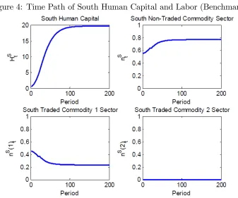
tax non-traded goods consumption and subsidize savings as shown in Figure 3. This shifts labor into the tradable sector and suppresses its overall consumption to increase exports. Figure 4 shows that the South government initially shifts labor into the tradable sector by suppressing consumption of non-traded commodity. As the South human capital grows through learning-by-exporting, it gradually raises its labor allocation to the non-traded com-modity sector and therefore its consumption. Figure 5 shows that the South government

25_{Data Source: BEA, World Development Indicators, and BLS Monthly Labor Review (July 2005).} 26_{Data Source: Penn World Table.}

27_{For instance, Park, Yang, Shi, and Jiang (2010) show that if a …rm experiences an exogenous 10%}

suppresses consumption of the export good (Traded Commodity 1) while reducing that of the import good (Traded Commodity 2) for the initial periods. This raises the South export, leading its human capital and real GDP to grow rapidly through learning-by-exporting as shown in Figures 4 and 6. The transition to the steady state takes 112 periods, during which the North produces both traded goods and the South produces the …rst traded commodity.28

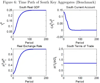
The initial pattern of export and import of the South causes the country to run a current account surplus, amid a rapid growth in its real GDP as shown in Figure 6.29 _{During the}

transition, the South terms of trade stay constant. Note that when one country produces both traded goods, the terms of trade are determined by its productivity ratio between two traded goods production. Since the North produces both traded goods for all periods, the South terms of trade are equal to the North productivity ratio between two traded goods p_pt(1)_t(2) = (H

N₎1+

HN . This is equal to the U.S. relative labor productivity of exporters

in 1992 (1:169). The constant South terms of trade makes the South real exchange rate appreciate as its human capital grows. This is because the South real exchange rate is a function of its terms of trade and relative productivity in traded commodity production

eS t

n

pt(1)

pt(2)

AS t(1)

AN₍₂₎

o1

. These simultaneous growth and real exchange rate appre-ciation are consistent with the Balassa (1964)-Samuelson (1964) hypothesis30_.

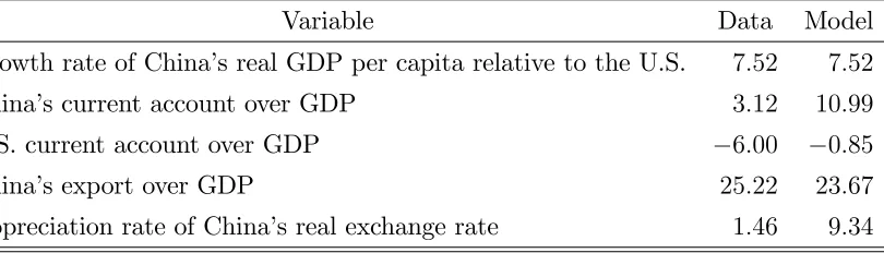
Table 2 summarizes the average values of key aggregates of the U.S. and China from 1991 to 2007 and their counterparts in the benchmark model. The model is calibrated to

28_{As I describe in Subsections 4.2, 4.3 and 5.2, the South produces the second traded commodity during}

the latter part of the transition in the "No Policy", "No-WTO Restrictions", and "Coordinated Policy" cases. This is because initially the South runs a substantial current account de…cit. In order to repay the interests on its debt, the South shifts more workers from non-tradable sector to both tradable sectors so that it runs a trade surplus for the rest of the transition periods.

29_{As can be seen in Figure 2, China’s current account surplus has increased over time. However, in this}

model, the South current account surplus is decreasing over time.

In the real world, the Chinese government could have gradually implemented policies to take advantage of learning-by-exporting. However, since this is a perfect foresight model, the South does not gradually implement policies. In order to match the trend, I should introduce some frictions like adjustment costs into this model.

30_{Balassa (1964) and Samuelson (1964) argue that economic growth driven by productivity gains in the}

match the average growth rate of China’s real GDP per capita relative to the U.S. (7:52%). As shown in Table 2, the South policies generate the simultaneous fast growth and current account surpluses observed in the data.31 _{In addition, the benchmark model replicates both}

China’s export over GDP and the appreciation of its real exchange rate as in the data.

4.2

No Policy Counterfactual

In the "No-Policy" economy, both …rms and workers know that the South human capital will grow over time but no one recognizes the law of motion for South human capital. Therefore, they do not have an incentive to raise the South export in order to take advantage of learning-by-exporting. If no policies were implemented in both the North and South countries, the transition to the steady state takes 118 periods as shown in Figure 7. This is 6 periods longer than that of the benchmark economy because no one implements policies to accelerate the South growth through learning-by-exporting in the "No-Policy" economy. During the transition, the patterns of specialization in production undergo three stages: (i) the North produces both traded goods and the South produces the …rst traded commodity for the …rst 96 periods; (ii) both countries are completely specialized in period 97; and (iii) the South starts to produce the second traded commodity in period 98.

Figure 7 shows that more South workers produce in the non-traded commodity sector for the initial 85 periods relative to the benchmark case, because the South labor productivity in the …rst traded commodity production is much less than that in non-traded commodity production over the same periods in the "No-Policy" world. This initially suppresses the South …rst traded commodity export although its consumption for the …rst traded commodity is less than in the benchmark economy as shown in Figure 8, delaying the take-o¤ of its human capital relative to the benchmark case.

31_{This model overstates China’s current account surplus and understates the U.S. current account de…cit.}

In the "No-Policy" economy, since the South workers know that their income will grow in the future, they want to raise current consumption. The South consumes more non-traded goods in the …rst 85 periods than in the benchmark economy, leading to a larger aggregate consumption. This makes the South current account de…cit32 _{increase for the same periods.}

The South workers move from non-tradable sector to both tradable sectors for the rest of the transition periods so that the South runs a trade surplus in order to repay the interests on its debt.33 _{Since more workers produce in both traded commodity sectors in the South country}

relative to the benchmark economy beginning in period 86, the level of South real GDP becomes greater than that in the benchmark case as Figure 9 presents. This is because labor productivity in the traded goods production is higher than that in non-traded commodity production over the same period. Figure 9 shows that the South terms of trade start to deteriorate in period 97 when both countries are completely specialized.34 _{Beginning in}

period 98 when the South produces both traded goods, its terms of trade, which are equal to the South productivity ratio (H

S t)

1+

HS

t ; improves as its human capital grows. For the

same period, the real exchange rate appreciates following the South human capital growth.

4.3

No WTO Restrictions

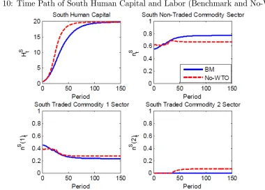
If there were no WTO restrictions EX

t 6= 0 , the South country can directly subsidize

exports. Figure 10 shows that the transition to the steady state takes 70 periods but the most catch-up takes place for the initial 50 periods. During the transition, the North produces both traded goods and the South produces the …rst traded commodity for the …rst 26 periods. As the South human capital grows, it gradually expands the world market share of the …rst traded commodity. In period 27, the South completely takes over the market for the …rst traded commodity, which leads to complete specialization of both countries until period 34.

32_{The size of the current account de…cits is implausible. This is caused by the full commitment and perfect}

foresight assumptions.

33_{The right panel of Figure 8 shows that the South exports even the second traded commodity from period}

100 in spite of a comparative disadvantage.

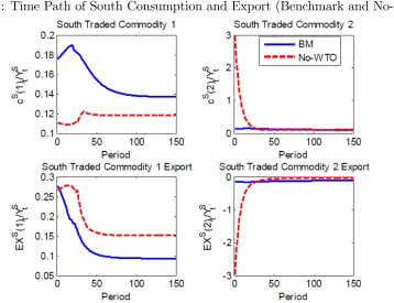
The South starts to produce the second traded commodity in period 35.

As shown in the left panel of Figure 11, the South government suppresses consump-tion of the export good (Traded Commodity 1) during the transiconsump-tion relative to benchmark outcomes. This raises the South export, making its human capital grow faster through learning-by-exporting relative to the benchmark economy. Figure 10 shows that the South government shifts more workers from the non-traded commodity sector to both traded goods sectors, than in the benchmark economy. Since labor productivity in both traded goods pro-duction is higher than that in non-traded commodity propro-duction, the level of South real GDP in "No-WTO Restrictions" case is greater than that in the benchmark economy beginning in period 11. The right panel of Figure 11 shows that the South substitutes the alternative import by raising consumption of the import good (Traded Commodity 2) substantially for the initial periods. As the South accumulates human capital through learning-by-exporting, its imports decline to the level which is even below that in the benchmark after period 35 when the South starts to produce the second traded commodity.

The increased South import initially causes the country to run a large current account de…cit. As the South import declines, the current account de…cit also goes down and ul-timately becomes balanced in the steady state. The South government’s export subsidy generates a deterioration in its terms of trade p_pt(1)_t(2) beginning in period 27 when both countries start to be completely specialized, as shown in the lower panel of Figure 12. When the North produces both traded goods for the initial 26 periods, the South terms of trade are equal to the North productivity ratio between two traded goods (H

N₎1+

HN , which is

time-invariant. When the South produces both traded goods beginning in period 35, its terms of trade are equivalent to its productivity ratio (H

S t)

1+

HS

t ; which rises with the South human

capital.

ideally the South would like to manipulate its terms of trade rather than its current account. However, if the ability to explicitly subsidize exports is absent due to the WTO restrictions, it must "over" distort both the intertemporal margin and the non-traded margin.

5

Coordinated Policy Problem

In this section, I consider a "Coordinated Policy" problem in which the North and South could coordinate policies, in order to obtain the …rst-best outcome for the world. I assume that there is a …ctitious world planner who maximizes the weighted average of both the North and South utilities by taking advantage of the South country’s learning-by-exporting. The world planner solves

max 1

X

t=0

t _u(CS

t) + (1 )u(C N t ) ;

subject to

HtS+1 =H

S

t + H N

HtS 1 exp

EXS t

;

ci t =n

i t; N

i _=ni t+n

i

t(1) +n i

t(2); i2 fN; Sg;

cSt(z) +c N

t (z) =A S t (z)n

S

t(z) +A N

(z)nNt (z);

nS

t(z) 0; n N

t (z) 0; z 2 f1;2g;

where 2[0;1]is the South country’s Pareto weight.

If the South country exports the traded commodity z 2 f1;2g, the world utility maxi-mizing behavior of the planner implies the following …rst-order conditions:

ucS t(z)

t HN HtS

exp EX

S t

= (1 )ucN

t (z); (2)

ucS t(z) A

S

t (z) = ucS

t 1; (3)

where t is a multiplier for the law of motion for South human capital, uci

t(z) is the country

i’s marginal utility of consumption for the traded commodity z; and uci

t is the country i’s

the left side of the condition (2), t( H

N _HS t)

exp EXSt _{; which appears due to}

learning-by-exporting, is positive. This implies that when the South country exports the traded commodityz, the world planner reduces the South country’s consumption for the exporting good cS

t(z) in order to take advantage of learning-by-exporting. The condition (3) shows

that there is no distortion between the South consumption for the export good and that of non-traded good. If a worker shifts from the non-traded commodity sector to the traded commodity z sector in the South country, this reduces one unit of non-traded commodity. Thus, the welfare loss is marginal utility of consumption for the non-traded commodity. However, the worker produces AS

t (z) units of the traded commodity z and by consuming

it, the worker can enjoy marginal utility of consumption for the commodity times marginal product AS

t (z) . Since the South country does not export the traded commodity z but

consumes it, there is no additional welfare gain from learning-by-exporting.35 _{The conditions}

(2) and (3) imply that the planner decreases not only the South country’s consumption for the export good but also that for non-traded good. This means that the planner raises the South exports by reducing its consumption of domestically produced goods and increasing consumption of the import good.

5.1

Decentralization

In this subsection, I explain the way I …nd prices and wedges, which imply the …rst-best allocation for the world. The North country’s non-traded commodity price is normalized to one. Since the North’s relative consumptions across goods are undistorted, I use their marginal rate of substitution between non-traded and traded goods as the world prices. The

35_{Note that non-traded goods consumption tax is needed in the presence of WTO restrictions. If a worker}

world pricept(z) of traded commodity z is de…ned by

pt(z)

ucN t (z)

ucN t

; z2 f1;2g;

where uci

t(z) is the country i’s marginal utility of consumption for the traded commodity z

anduci

t is the countryi’s marginal utility of consumption for its non-traded commodity. The

world interest ratert+1 is de…ned by

rt+1

ucN t

ucN t+1

1:

Since the South country has a comparative advantage in the …rst traded commodity pro-duction, it produces the …rst traded commodity and the North produces the second traded commodity. Therefore, the South domestic wage is de…ned by

wtS

pt(1)

pt(2)

AS t (1)

AN₍₂₎ =p S t:

A wedge r

t+1 in the South country’s domestic interest rate, a wedge EXt in the South

domestic relative price of export good to import good, and a wedge N T

t in the South

domestic relative price of export good to non-traded good are de…ned by

r t+1

wS t+1 ucS

t

rt+1 wtS ucS t+1

1

rt+1

1 () w

S t+1 ucS

t

wS

t ucS t+1

1 = 1 + rt+1 rt+1;

EX t

pt(2) ucS t(1)

pt(1) ucS t(2)

1 () ucSt(1)

ucS t(2)

= 1 +

EX t pt(1)

pt(2)

;

N T t

ucS t

AS

t (1) ucS t(1)

1 () ucSt(1)

ucS t

= pt(1) (1 + N T

t )pSt

= 1

(1 + N T

t )ASt (1)

:

5.2

Results

I use the same parameters for the "Coordinated Policy" case as in the benchmark economy, except for the South Pareto weight = 0:3314 which is chosen so that the model matches the balanced steady state current account.36

When both the North and South coordinate policies to achieve the world best allocation, the transition to the steady state takes 64 periods as Figure 14 presents. This is 6 periods

36_{If is greater than0:3314, the South runs a current account de…cit at the steady state. If is less than}

less than that of "No-WTO Restrictions" economy because the world planner facilitates growth through terms of trade distortion even more. During the transition, the patterns of specialization in production undergo three stages as before: (i) the North produces both traded goods and the South produces the …rst traded commodity for the …rst 24 periods; (ii) both countries are completely specialized from period 25 to 34; and (iii) the South starts to produce the second traded commodity in period 35. The …rst stage gets shorter relative to the "No-WTO Restrictions" case.

The left panel of Figure 15 shows that the world planner reduces the South consumption of the export good (Traded Commodity 1) even more from period 19 than in the "No-WTO Restrictions" economy. This increases the South export, making its human capital grow more rapidly through learning-by-exporting than in the "No-WTO Restrictions" case. As can be seen in Figure 14, the world planner moves more workers from non-traded commodity sector to both traded commodity sectors in the South country relative to the "No-WTO Re-strictions" economy beginning in period 25. This makes the level of South real GDP greater than that in "No-WTO Restrictions" case over the same period because labor productivity in the traded goods production is higher than that in non-traded commodity production. The right panel of Figure 15 shows that, for the initial periods, the world planner raises the South import by 43% of its GDP relative to the "No-WTO Restrictions" world by increasing its consumption of the import good (Traded Commodity 2).

undervaluation contrast with the prediction of the Balassa (1964)-Samuelson (1964) hypoth-esis. When the South produces both traded goods beginning in period 35, its terms of trade

pt(1)

pt(2) =

(HS t)

1+

HS

t improve due to the growth of South human capital. For the same period,

the real exchange rate appreciates following the real GDP growth. This implies that the world planner postpones the Balassa (1964)-Samuelson (1964) e¤ect by deteriorating the South terms of trade.

Figure 17 shows that the world planner uses a bigger export subsidy and a less saving subsidy relative to the "No-WTO Restrictions" case. This implies that the world planner calls for more terms of trade manipulation than the No-WTO policies.

6

Welfare Analysis

This paper explores optimal policies in the presence of learning-by-exporting in various environments: with the WTO restrictions, with no restrictions, and under the policy coordi-nation. An interesting question is what are the welfare consequences of those policies for the developing and developed economies. In order to answer this question, I measure the welfare changes due to moving from the benchmark economy with the WTO restrictions to another environment using the percentage change in per-period consumption that I should give to the worker in each country in the benchmark so that the worker is indi¤erent between the two environments.

of the policy implemented in the benchmark economy is measured by welfare changes from the benchmark economy to the "No-Policy" world in Table 3. These welfare changes are equivalent to19:10%decline and0:06%increase in per-period consumption of the South and the North, respectively.

If the South country is allowed to manipulate its terms of trade ("No-WTO Restrictions" case), both the North and South bene…t from welfare improvement relative to the benchmark economy. Without restrictions on the policies, the South country subsidizes exports to reduce its consumption of the export good and increase consumption of the import good. This policy generates a large deterioration in the South terms of trade and a current account de…cit. These policies make the South grow faster without raising savings heavily to promote exports, which improves the welfare of the South relative to the benchmark economy. In the "No-WTO Restrictions" world, the North welfare also increases due to improved terms of trade compared with the benchmark economy. This "win-win" outcome through the terms of trade manipulation is re‡ected in the welfare gains of 14:08% and 0:43% rises in per-period consumption of the South and the North, respectively. This contrasts with Bagwell and Staiger (1999)’s view that the WTO improves the world welfare by preventing zero-sum terms of trade manipulation.37

As shown in Table 3, if both countries coordinate policies to achieve the world best al-location, both countries’ welfare rises signi…cantly compared with the benchmark economy. The …ctitious world planner manipulates the terms of trade of both countries so that the South grows faster through learning-by-exporting. This leads to the welfare gains equivalent to 13:24% and 1:16% increases in per-period consumption of the South and the North, re-spectively. However, moving from the "No-WTO Restrictions" economy to the "Coordinated Policy" world, the North is better o¤ whereas the South is worse o¤. The world planner pulls down the relative price of the South export good to its import good even more than in the

37_{There may be other reasons that the WTO restrictions improve the welfare of developing countries.}

"No-WTO Restrictions" economy. Even though this makes the South country grow faster, the larger deterioration of the South terms of trade hurts its welfare. On the other hand, the North bene…ts from its improved terms of trade. However, the welfare changes of both countries between "No-WTO Restrictions" case and the "Coordinated Policy" economy are quantitatively modest.

7

Sensitivity Analysis

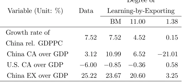
I do a sensitivity analysis on the degree of by-exporting. The degree of learning-by-exporting is measured by a rise in a …rm’s productivity accompanied by a 10% increase in exports. According to Park, Yang, Shi, and Jiang (2010), a …rm’s productivity increases by11% to13% in China, if it experiences an exogenous 10% rise in exports. Table 4 shows that if I use the lowest value of the micro estimate on the degree of learning-by-exporting, which is11%, the benchmark model still generates the simultaneous fast growth and current account surplus of the South country. However, the levels of both the average growth rate of China’s real GDP per capita relative to the U.S. and China’s current account over GDP decrease relative to the benchmark calibration in which the degree of learning-by-exporting is 12:91%. If the degree of learning-by-exporting is about one tenth of the highest value of micro estimate, that is, 1:38%, the South does not need to run a current account surplus to take advantage of learning-by-exporting. This result shows that the cross-country di¤erences in the degree of learning-by-exporting may explain the heterogeneity in the pattern of current account across developing countries.

8

Conclusion

rest of the world, and if restricting the set of policies to non-trade related policies matter. In order to answer these questions, this paper builds a two country general equilibrium growth model in which a developing economy bene…ts from learning-by-exporting as it trades with a developed economy. If the policies are restricted to non-trade related ones by the WTO, the optimal policy for the developing country is to tax non-traded goods consumption and subsidize savings, which rationalize the observed current account surpluses of rapidly growing developing economies. This policy improves the welfare of developing country rela-tive to a "No-Policy" competirela-tive equilibrium.

If there were no WTO restrictions, the developing country directly subsidizes exports. This policy generates a large deterioration in the developing economy’s terms of trade and reverses the prediction for the current account. This policy raises the welfare of both coun-tries relative to the model with WTO restrictions, as it generates faster economic growth in the developing economy and improvement of the terms of trade in the developed economy. This paper also considers a “Coordinated Policy” problem to obtain the …rst-best outcomes for the world. In this setup, the developing country’s terms of trade deteriorate even more and it runs a greater current account de…cit relative to the “No-WTO Restrictions” case.

Appendix

A Derivation of the Implementability Condition

The North representative worker solves:

max 1

X

t=0

t

u(CtN);

subject to 1 X t=0 t Y i=0 1 1 +ri

!

1 cNt +pt(1) ctN(1) +pt(2) cNt (2) 1 N N

=bN₀ : (4)

The worker’s …rst order conditions are:

ucN t+1

ucN t

= 1

1 +rt+1

;

ucN t (z)

ucN t

= pt(z); z 2 f1;2g:

Plugging the above …rst order conditions into the North worker’s present-value budget con-straint (4) yields

1 X t=0 t Y i=1

ucN i

ucN i 1

!

1 cNt +

ucN t (1)

ucN t

cNt (1) +

ucN t (2)

ucN t

cNt (2) 1 N N

!

=bN₀ :

Since ucN

i ’s; i2 f1;2; ; t 1g are canceled out in

t Y i=1 u_cN i u

cN_{i 1}

!

, I have

1

X

t=0

t

ucN t

ucN 0

!

1 cNt +

ucN t (1)

ucN t

cNt (1) +

ucN t (2)

ucN t

cNt (2) 1 N N

!

=bN0 : (5)

Multiplying both sides of equation (5) byucN

0 , I obtain the implementability condition

1

X

t=0

t

ucN t c

N t +ucN

t (1) c

N

t (1) +ucN t (2) c

N

t (2) ucN t N

N _=u cN

0 b

N

0 : (6)

B Computation Algorithm

The following algorithm is used to solve the benchmark model.

2. Given and bN

0 = 0, solve the following value function using value function iterations

and obtain the optimal decision rules:

V(HtS; )

max

2

4 u(C

S

t) + ucN t c

N t +ucN

t (1) c

N

t (1) +ucN t (2) c

N

t (2) ucN t N

N

+ V(HS t+1; )

3

5;

subject to

HS

t+1 =HtS+ H

N _HS

t 1 exp

EXS t _;

Ni _=ni t+n

i

t(1) +n i t(2); c

i t =n

i

t; i2 fN; Sg;

cNt (z) +c S

t(z) =A N t (z)n

N

t (z) +A S t (z)n

S t(z);

ucN t (z)

ucN t

1

AN t (z)

; nN

t (z) 0; n S

t(z) 0; z2 f1;2g;

ucS t(1)

ucS t(2)

= ucNt (1)

ucN t (2)

:

3. Using the optimal decision rules, simulate for a transition to a steady state.

References

Aguiar, M., and M. Amador (2011): “Growth in the Shadow of Expropriation,”

Quar-terly Journal of Economics, 126(2), 651–697.

Aw, B. Y., M. J. Roberts, and D. Y. Xu (2010): “R&D Investment, Exporting, and

Productivity Dynamics,”American Economic Review, Forthcoming.

Bagwell, K., and R. W. Staiger (1999): “An Economic Theory of GATT,” American

Economic Review, 89(1), 215–248.

Bajona, C., and T. Chu (2010): “Reforming State Owned Enterprises in China: E¤ects

of WTO Accession,”Review of Economic Dynamics, 13(4), 800–823.

Balassa, B. (1964): “The Purchasing Power Parity Doctrine: a Reappraisal,” Journal of

Political Economy, 72(6), 584–596.

Bernard, A. B., and J. B. Jensen (1999): “Exceptional Exporter Performance: Cause,

E¤ect, or Both?,”Journal of International Economics, 47(1), 1–25.

Blalock, G., and P. J. Gertler (2004): “Learning from Exporting Revisited in a Less

Developed Setting,”Journal of Development Economics, 75(2), 397–416.

Caballero, R., E. Farhi, and P.-O. Gourinchas (2008): “An Equilibrium Model of

"Global Imbalances" and Low Interest Rates,” American Economic Review, 98, 358–393.

De Loecker, J. (2007): “Do exports generate higher productivity? Evidence from

Slove-nia,”Journal of International Economics, 73, 69–98.

(2010): “A Note on Detecting Learning by Exporting,” NBER Working Paper No. 16548.

Fernandes, A. M., and A. E. Isgut (2009): “Learning-by-Exporting E¤ects: Are They

Fogli, A.,and F. Perri(2006): “The Great Moderation and the US External Imbalance,”

Monetary and Economic Studies, 24, 209–225.

Gourinchas, P.-O., and O. Jeanne (2009): “Capital Flows to Developing Countries:

The Allocation Puzzle,” Mimeo.

Guo, S., and F. Perri (2010): “The Allocation Puzzle Is Not As Bad As You Think,”

Mimeo.

Harrison, A., and A. Rodríguez-Clare (2010): “Trade, Foreign Investment, and

In-dustrial Policy for Developing Countries,”Handbook of Development Economics, 5, 4039– 4214.

Jones, L. E., R. E. Manuelli, and P. E. Rossi (1997): “On the Optimal Taxation of

Capital Income,” Journal of Economic Theory, 73(1), 93–117.

Keller, W.(2004): “International Technology Di¤usion,”Journal of Economic Literature,

42(3), 752–782.

Kraay, A. (1999): “Exportations et Performances Economiques: Etude d’un Panel

d’Entreprises Chinoises,” Revue d’Economie Du Developpement, 1-2, 183–207.

Ma, G., and W. Yi (2010): “China’s High Saving Rate: Myth and Reality,” BIS Working

Papers No. 312.

Mendoza, E. G., V. Quadrini, and J.-V. Rios-Rull (2009): “Financial Integration,

Financial Development and Global Imbalances,” Journal of Political Economy, 117(3), 371–416.

Park, A., D. Yang, X. Shi, and Y. Jiang (2010): “Exporting and Firm Performance:

Ping, X., S. Liang, C. Hao, H. Zhang, and L. Mao (2009): “Studying on the Welfare E¤ects of VAT and Business Tax,”Economic Research Journal, 44(9), 66–80 [in Chinese].

Samuelson, P. A. (1964): “Theoretical Notes on Trade Problems,” Review of Economics

and Statistics, 46(2), 145–154.

Song, Z., K. Storesletten,and F. Zilibotti(2011): “Growing Like China,”American

Economic Review, 101(1), 202–241.

Song, Z. M., and D. T. Yang(2010): “Life Cycle Earnings and Saving in a Fast-Growing

Economy,” Mimeo.

Stockman, A. C., and L. L. Tesar (1995): “Tastes and Technology in a Two-Country

Model of the Business Cycle: Explaining International Comovements,” American Eco-nomic Review, 85(1), 168–185.

Van Biesebroeck, J. (2005): “Exporting Raises Productivity in Sub-Saharan African

Table 1: Parameter Values of the Benchmark Model Economy Parameter Description

= 0:96 Discount factor

1= = 0:5 Intertemporal elasticity of substitution

= 0:2438 Expenditure share on traded goods

= 0:5516 Expenditure share on the …rst traded commodity ( ) = 0:99 South human capital at the steady state HN

= 0 Degree of learning-by-exporting from the second traded commodity export

NN _{= 1 The North country’s labor}

NS _{= 1 The South country’s labor}

bS

0 = 0 The South country’s initial debt

HS

0 = 0:5269 The South country’s initial human capital

HN _{= 19:8941 The North country’s human capital}

= 0:0522 Labor productivity in the second traded commodity production

= 33:8927 Degree of learning-by-exporting

Table 2: Average of Aggregate Variables from 1991 to 2007 (Unit: %) Variable Data Model Growth rate of China’s real GDP per capita relative to the U.S. 7:52 7:52

China’s current account over GDP 3:12 10:99

U.S. current account over GDP 6:00 0:85

China’s export over GDP 25:22 23:67

Table 3: Welfare Gain or Loss (Unit: Per-Period Consumption) South North Benchmark =) No Policy 19:10% +0:06%

Benchmark =) No WTO +14:08% +0:43%

Benchmark =) Coordinated Policy +13:24% +1:16%

No WTO =) Coordinated Policy 0:74% +0:73%

Table 4: Impact of Degree of Learning-by-Exporting

Variable (Unit: %) Data

Degree of

Learning-by-Exporting BM 11:00 1:38

Growth rate of

China rel. GDPPC 7:52 7:52 4:52 0:15 China CA over GDP 3:12 10:99 6:52 21:01

U.S. CA over GDP 6:00 0:85 0:36 0:58

Figure 1: China’s Exports and Economic Growth

Figure 3: Time Path of South Tax and Subsidy (Benchmark)

Figure 5: Time Path of South Consumption and Export (Benchmark)

Figure 7: Time Path of South Human Capital and Labor (Benchmark and No-Policy)

Figure 9: Time Path of South Key Aggregates (Benchmark and No-Policy)

Figure 11: Time Path of South Consumption and Export (Benchmark and No-WTO)

Figure 13: Time Path of South Tax and Subsidy (Benchmark and No-WTO)

Figure 15: Time Path of South Consumption and Export (Benchmark, No-WTO, and Co-ordinated Policy)