After ten years the Russian crisis how IMF intervention might be evaluated?

Munich Personal RePEc Archive

AFTER ten years the Russian crisis how

IMF intervention might be evaluated?

Sulimierska, Malgorzata

University of Sussex, Department of Economics

29 April 2011

Online at

https://mpra.ub.uni-muenchen.de/30930/

After ten years the Russian crisis how IMF intervention might be evaluated ?

Malgorzata Sulimierska

Economics Department, University of Sussex, Brighton BN1-9RH, England LICOS, Centre of Transition Economics, Economics Department, Katholieke

Universiteit Leuven, Debériotstraat 34, 3000 Leuven, Belgium E-mail: [email protected]

Abstract

The ongoing global financial crisis has become prominently visible since September 2008. This crisis affected the whole world and enhanced the importance of policy implementation to mitigate financial crises in future. Many academics blamed insufficient domestic regulation as the reason of crises, others pointed to the lack of overseas financial regulation and inappropriate actions by international organizations, such as the IMF and World Bank. This whole discussion encouraged to look back and analyzed a previous crisis in smallest countries such as Russia. This paper evidently shows the inefficiency of IMF policy during the Russia Crisis in 1998 by implementing a new monetary balance-of-payment model in Russian data. This model identified the role of macroeconomic fundamentals and international economic policy implications on the likelihood and the timing of the currency crisis in Russia. For the period from December 1995 to December 1998 it was found that, the increase in domestic credit growth gradually undermined confidence in the fixed exchange rate regime. The most dangerous point was at the end of 1998, when the collapse probability was above 90 percent. This result ambiguously questioned the IMF’s July packet 1998 and proved the political aspects of this financial help.

Keywords: currency crisis, financial liberalization, sudden-stops, monetary

balance-of-payment model, Russian crisis, IMF’s policy

Acknowledgements

1. Introduction

economy to face a currency crisis after so much had been accomplished and what was the impact of IMF intervention on Russian crisis?

It seems natural to analyse in this paper the reasons for the Russian crisis and explain the IMF’s impact on this crisis. In order to explain this, three aspects will need to be analysed. Firstly, how theoretical studies might explain the Russian currency crisis. Secondly, whether this crisis could have been predicted in theoretical terms or whether the crisis might have been inevitable, and lastly, but not least, how can the impact of difficult external intervention, especially by the IMF, on the crisis be understood? It is not possible to leave out of the account the impact of the IMF intervention on the Russian economy and investors’ expectations.

This paper is divided into four parts. The first part describes the theoretical basis of the currency crisis though various generations of models. Then the second part presents the empirical literature review, especially the analysis of a single country. In the last part, the Russian case is described in order to adopt the empirical econometric model, in which I modified CVW’s model (a monetary balance–of-payments model) (Cumby and Van Wijnbergen’s model). This modification answers the question of whether the crisis could have been predicted. The section discusses the role of the IMF in the Russian crisis.

2. Theoretical models of currency crises

market agents start doubting the ability of the central bank to control the fixed exchange rates system. Then reserves fall to a critical threshold, the rational agents initiate speculative attacks on the foreign exchange which lead to the collapse of the exchange rate (see Krugman (1979), Salant and Henderson (1978), Dornbush (1987) and Flood and Garber (1984), Flood, Garber and Kramer (1996)).

this future government policy and then start the actions that affect some variables (e.g. interest rate) and wait for economic policies to respond. In that case, the level of reserve will mainly depend on the degree of commitment of authorities to hold the peg. The weaker the commitment of the authorities the higher the probability that the speculative attack will be successful (see Obstfeld (1986a,b, 1994) Ozkan and Sutherland (1995), Reisen (1998) and Krugman (1996)).

The pure speculation models have two interesting tales to be told. The first tale describes the speculation against the currency as the consequence of herding behaviour (Calvo and Mendoza (2000), Binkhchandani and Sharma(2000)). Then the second tale gives large attention to the contagion and sudden stops effects (Gerlach and Smets (1995), Eichenngreen, Rose, Wyplosz (1996), Masson (1998)).1 There are two different ways to present the herding behaviours. Firstly, full information assumption does not hold, agents have different pieces of information due to the cost of information. In order to reduce this cost, individuals start to base their behaviours on the behaviours of others (so-called leaders). This might move financial market to an ineffective distribution and then to a crisis outcome (Calvo and Mendoza (2000)). Secondly, the manager’s salary will not decrease so much if the other investors on the market make the same mistake. In that situation the cost of standing out against other portfolio managers’ crowd is larger than followed wrong along with everyone. (Binkhchandani and Sharma(2000)).

The last story about crisis, the so-called third generation model of currency crisis, has been developed rapidly soon after the Asian crisis. This crisis could not be explained by previous theoretical models and moved

1_{The contagion and hedging effects is considered as the part of the second-generation models}

attentions to micro fundamentals of an economy (see Krugman (1998, 1999 a,b) and Velasco (2001)). The third generation models consider three micro fundamentals of an economy as reasons of the currency crisis:

-fragility of banking system (McKinnon and Huw Pill(1996), Chang and Velasco (1998 a, b, c), Kaminsky and Reinhart (1999));

-financial market inefficiency (moral hazard or the problem of asymmetrical information) (see Stoker (1994), Mishkin (1996) Krugman (1998))

-companies’ balance sheet and the effects of monetary policy (see Krugman (1999 a,b), Aghion, Bacchetta and Banerjee (2000,2001),Borenszten and Lee (2000), Coulibaly and Millar (2008))

The first issue addressed in the development of third generation models were the fragility of the banking system and financial market inefficiency. The discussion might be started at the modern variants of the first generation model, the so-called twin banking-currency crisis model (Glick and Hutchison (2001)). This framework stresses the fact that currency crises are often part of broader financial crises, where the two elements interact with one another, giving life to what have been called the “twin crises”.2 These models suggest that when central banks finance the bailout of troubled financial institutions by printing money and open the economy with exchange rate peg, there is the classic story of a currency crash prompted by excessive money creation (see Stoker (1994), Mishkin (1996)) Krugman (1998, 1999a,b), Kaminsky and Reinhart (1999)). After that, Chang and Velasco (1998 a, b, c) investigated more intensely the aspects of the financial fragility and currency crisis. In opened economy

2 _{The twin banking-currency crisis model relies on the Diamond and Dybvig‘s dilemma (1983).}

models, the banks play active role, not only as distributor of deposits, but also generating large capital inflows to the economy though borrowing money from aboard at a low interest rate and then reinvest in the domestic market. But at the same time it creates the risk of a sudden reversal of capital flows and international illiquidity3 of the domestic financial system. For instance, if depositors will attempt to withdraw funds in the short run and then foreign creditors will not roll over initial credit in the short run. In that case, the bank will not be able to honour all of its commitments. The domestic banks do not have enough domestic deposits in liquid form. Long-term investments of the domestic bank will yield little if they have to be liquidated prematurely. The central bank plays the role of a lender of the resort in the opened economy with a fixed exchange rate. However, the stability of banking system is depended on the size of the central bank’s reserves and the exchange rate regime strength. On the other hand, to support domestic banks, the central bank might pursue an expansionary policy and keep interest rates from rising. But still, private agents use the additional domestic currency to deplete the central bank’s reserves. Therefore with limited international reserves, eventually, the central bank will abandon the peg. This shows how a financial crisis can transfer to a balance of payments crisis and caused boom-bust cycles. The further expansion of borrowing abroad by domestic banks creates the lending expansion and investing-consumption booms in the domestic economy. These booms might continue to widen the current account deficit and then financial markets will need more foreign capital to feed the trade deficit (Kaminsky and Reinhart (1999:475). Moreover, the lending boom converge levels gradually in inflation and then cumulative real exchange rate appreciation (see

3_{The key issue is a mismatch of assets and liabilities: a country's financial system is}

Dornbusch(1976,1987)’s overshooting model ). Cumulative real exchange rate appreciation generates the expectation of exchange rate depreciation on the market. Change and Velasco’s model point out that the capital inflows become outflows and cause the collapse of the banking system causing currency crisis.4 Finally, the last branch of the third generation models concentred on a problem appears in balance sheet firms as the primary source of crises. Especially, Krugman (1999 a, b) and Aghion, Bacchetta and Banerjee (1999, 2001) intensively investigated this topic though its connection to other microeconomics aspects such as fragility of the banking system and asymmetrical information (moral hazard). In the models, the crisis might happen under different exchange rate regime. The entrepreneurs obtained credits from two sources: domestic or foreign markets. It allowed them to mix short-term debt, denominated in domestic currency and long-term debt denominated in foreign currency. The credits amount to finance investment depends on firms’ wealth. And on the other hand, the firms’ wealth primarily determines investment and output (Bernanke and Gertler (1989). In the case of any economic shock, the sudden capital inflows cause an explosion in the domestic currency value of dollar debt and in this manner increased in foreign currency repayments and reduce their ability to borrow for further investments. Moreover the decline of investment and output implied a credit-constrain in economy. Further reduction of capital inflows decreases the demand for the domestic currency and leads to depreciation. Thus, the financial crisis cycles started to close circle (Aghion, Bacchetta and Banerjee (2001).

In the end, it is worth talking about Sudden –Stop Models (see Calvo (1998), Mendoza (2001), Mendoza and Smith (2002) and Hutchison and Noy

4 _{To provide unambiguous evidence to support the theory on the causal links between currency}

(2002), Calvo, Izquierdo and Mejia (2004), Valdes (2008)). These models analysed a phenomenon of abrupt reduction of the capital inflows into a country. Before the moment of abrupt reduction it has been receiving large volumes of foreign capital. But they focused on micro and macro perspective so they are in the middle between second and third generation models.

3. Overview of empirical literature

A large number of empirical studies have examined the determinants of currency crises, but the empirical evidence is far from conclusive inference. In general, two lines of analysis can be distinguished: single-country or multi-single-country. The number of multi-countries has grown rapidly since the beginning of 1990s (see Sulimierska (2008b)). However, these multi-country analyses have some limitations due to attempt to exploit the higher variability associated with cross-country information. In that way, the evidence from multi-country studies is mixed and not very robust contrast to single-country studies (Esquivel and Larrain (1998:9)). On the other hand, the most of single-country studies were developed before 1990s. However, after the Asian Crisis academic attention moved back to single country analysis by investigating microeconomic fundaments such as company’s debts, performance of financial institutions (see Borenszten and Jong-Wha (2000)).

devaluation in a specific country based on the behaviour of several macroeconomic indicators (the linear discrete time models). Most of them have generally found strong evidence suggesting that domestic macroeconomic indicators play a key role in determining currency crises. Nevertheless, these results might be suggestive, are sometimes limited since they are obtained from a small number of countries during very specific situations.5

However, both studies above provide evidence for qualitative success of applying first generation model (the linear discrete time models) although these results can be broadly discussed since the restrictive assumptions including the purchasing power parity (PPP), interest rate parity, and the unresponsiveness of the demand for real balance to currency substitution motives (see CVW (1989), Blanco and Garber (1986), Goldberg (1994). Both models state that domestic credit shocks are still expected to be the dominant force in triggering speculative attacks on currency.

In briefly summarizing the first generation empirical literature is necessary to start with the classic representation Blanco and Garber (1986) model. This model analysed the movement from one fixed exchange rate to another and computed the one-period ahead collapse probability for the fixed Mexican peso exchange rate from 1973-1982. To obtain these results they produced the devaluation models and used the time-series estimates of the one-period -ahead probability of devaluation that allowed them to predict the timing, probability of speculative attacks and forecast lower bounds for the post-collapse exchange rates. Blanco and Garber’s model is a version of Krugman –Flood-Garber model. In this model, Blanko and –Flood-Garber took the forward exchange rate as the shadow exchange, fixed exchange rate and calculation of the economic

5 _{This overview neglects the empirical models of currency crisis which consider different aspect}

fundamental from the bubble model and to construct new regime of fixed exchange rate after currency crisis. The results of this paper showed that large exchange rate adjustments in Mexico were preceded by substantial increases in the ex-ante probability of devaluation. It is strong evidence of the first generation views of currency crisis; however their model replicates some aspects of the relatively high values prior to actual devaluation. This causes some critics that exchange rate policy could not acknowledge an eventual devaluation ,and then a crawling peg will be though be equivalent to a fixed exchange rate regime after speculative attack because (see Reynoso (2002b)).

A subsequent study along this line is CVW’s paper (1989). It is a similar model to Blanco and Garber’s (1986) model with crawling exchange regime. On the contrary to Blanco and Garber ‘s (1986), the domestic credit is not followed the stochastic process. Furthermore, the central bank does not know the critical level of international reserve at which the exchange rate regime will abandon before the speculative attacks. Because of this, authorise assumed the reserve floor was describe by a uniform distribution with an upper bound as the current level of reserves and the lower bound as minus the central bank’s gross foreign liabilities. The final conclusion from model is that the domestic credit growth strategy pursued by the Argentine government almost completely undermined the announced crawling peg exchange rate

Nevertheless there are some modifications compare with previous papers due to the author used the Goldberg (1991) version of Flood and Garber’s model (1984) as the base of estimation model (1995). As before the domestic credit creation and domestic spending excess are viewed as the primary reasons for reserve depletion. If, in any period, expansion of domestic credit is too large to be absorbed by the demand for real balance, equilibrium in the money market is achieved in tow way. The first way is though adjustment of the exchange rate in a flexible exchange rate system. The way is by offsetting movements in central bank foreign exchange reserve stocks in controlled exchange rate system. In order that the discrete -time collapsing exchange rate model relies in a money market equilibrium condition which determines either the equilibrium exchange rate under a flexible exchange rate system or the endogenous path of central bank reserve under a controlled exchange rate system. In accordance with the paper’s results domestic fiscal and monetary shocks were the main forces contributing to speculative attacks on the Mexican peso. Furthermore, the result suggested that the external credit shocks played a relatively minor role in the onset of Mexico’s currency crises during the 1980s. Moreover, a reduction of domestic credit growth increases the uncertainty surrounding this growth. Then, there will be reduction of the size and perhaps increase the frequency of currency realignments which might have greatly reduced the amount of currency speculation against the peso between 1980 and 1986.

committed to maintaining the exchange rate within some form of crawling exchange rate regime in of a small open country. This model estimates the probability of devaluation to capture the systematic relationship between the realised regime changes and economic fundamentals. This probability evaluates whether speculative pressures on the currency can be accounted for by economic fundamentals. Formally, the one-step-ahead probability of a regime change can be approximated by computing the probability that the floating exchange rate next period will exceed the prevailing fixed exchange rate. In order to distinguish the determinants of the likelihood of a currency crisis or the timing of crisis they used the survival model. In accordance with the empirical findings the probability associated with all regime changes in the sample period can be attributed to speculative pressures in light of some deterioration in economic fundamentals. In addition these results suggested that the decline in foreign reserves, the increase in the share of short-term foreign currency-indexed debt, and /or expansionary monetary and fiscal policies seem to be the main factors which determined the timing of speculative attacks Pazarba io lu and Ötker (1997:841-845).

4. Empirical part: The Russia Econometric model

4.1. The Russian Case study

This section provides a brief review of the Russia economic and political situation in the late 1990s (Appendix A Table 1) that prompts some of the questions addressed in the theoretical model in the next section.

However, this was a period of significant political instability. Government offices were taken over by the young reformers, medium-level Communist Party members who were promoted to high level government positions, but who knew little about politics and economics Ivanova and Wyplosz (2000:15-16). They were unable to create new democratic and economic institutions within the framework of the old communist and corrupt Russian environment. The last pillar was massive privatisation to create a new capitalist class to protect the new democratic capitalist structure, but, instead, it created an oligarchy.6 Within a year of its rebirth, Russia was in complete disarray. Inflation was out of control, the federal budget was quickly contracting, damaging basic public services. The standard of living sharply declined, and Mafia of all sorts had established themselves. The threat of the return of communism increased due to Yeltsin’s waning popularity and the rebuilding of the communist party in a new form under Genna (Ivanova and Wyplosz (2000:16).) To an extent, all these negative economic and political events culminated in the currency crisis of ’’Black Tuesday’’, on 11th October 1994. However, the collapse of the economy allowed the start of a new program of mass privatisation and a successful disinflation program partly based on anchoring the rouble to the dollar though a crawling peg

6

arrangement, the corridor. In July 1995, this disinflation program was adopted by tightening monetary policy by giving autonomy to the Central Bank of Russia (Sutale (1999:7), Małecki, Sławi ski, Piasecki and uławska (2001:137-153)).In addition, after Yeltsin’s re-election in 1996, international optimism increased. In April 1996, Russian officials began negotiations to reschedule the repayment of the foreign debt inherited from the former Soviet Union as members of the Paris and London Clubs of indebted nations and international institutions became obligated to expand their assistance.7 Clearly, the outlook in 1997 presented good reasons for optimism. Russian politics had managed to establish most of the pre-conditions for a successful transition, but they had failed in some important details due to impossible political conditions. Mass privatisation is usually presented as an unmitigated disaster.8 However, there were many positive signals. Inflation was no longer a debilitating factor. The inflation rate for 1997 stood at 11 percentages, down from 2500 percentage in 1992. Monetary policy was entirely dedicated to the pursuit of disinflation, aiming at a rate of 5 percentages by the end of 1998. The exchange rate had been brought into the corridor in July 1995, and was successfully kept in a narrow band between 5 and 6 roubles to the Dollar (Appendix A Figure 3).The trade balance never posed

7 _{The World Bank was prepared to provide expanded assistance of $2 to $3 billion per year. The}

International Monetary Fund (IMF) continued to meet with Russian officials and provided aid. In September 1997, Russia was allowed to join the Paris Club of creditor nations after rescheduling the payment of over in old Soviet debt to other governments. Moreover, Russian government singed another agreement for debt repayment with the London Club. However, the improvement of international credit rating can be very questionable. For example, the Paris Club’s recognition of Russia as a creditor nation was based upon discussible qualifications. The one-fourth of the assets considered to belong to Russia was in the form of debt owed to the former Soviet Union by countries such as Cuba, Mongolia, and Vietnam. The recognition by the Paris Club was also based on the old, completely arbitrary official Soviet exchange rate of approximately 0.6 rubles to the dollar. The improved credit ratings Russia received from its Paris Club recognition were not based on an improved balance sheet ( Chiodo and Owyang (2002 :11), Stiglitz (2000:15-19)

8 _{In 1997, 69 percentages of enterprises were private (including foreign ownership), 9 percentages}

any threat (Appendix A Figure 4). Oil, gas and mineral exports were virtually guaranteed, at least in volume. This allowed Russia to purchase western goods deemed superior in quality. Following liberalisation, imports had risen sharply while non-oil, non-mineral, non-military imports and exports were insignificant. Russian manufacturers were largely unable to complete orders for their own domestic markets, far less for foreign markets (Chiodo and Owyang (2002: 11), Ivanova and Wyplosz (2000:17-19)).

result in conflicting incentives for regional governments and lead them to help firms conceal part of their taxable profit from the federal government in order to reduce the firms’ total tax payments. In return, the firm would then make transfers to the accommodating regional government (a kind of barter trade). This can explain why federal revenues dropped more rapidly than regional revenues (Desai, (2000:49), Shleifer and Treisman (2000:100-149)).

direct contract or via the banking system. Of the CBR and Sberbank (the largest State Saving Bank), which held about 50 percent of GKOs, assisted the government by purchasing new GKO issues at the primary auctions. The remaining GKOs were held by the domestic commercial banks, owned by the oligarchs. The OFZ’s market did not develop so dynamically because of investor uncertainty (Ivanova and Wyplosz (2000:33)).

But the glimpse of recovery seen in 1997, when Russia became the lowest-risk member of the world market according to her international credit rating and with greater domestic stability, was not to last long. The international situation of the foreign market was badly hit by the East Asian crisis in the summer of 1997, and in November 1997, the rouble came under speculative attack. The Central Bank of Russia defended the currency by reducing its foreign-exchange reserves. At the same time, non-resident holders of short-term government bills (GKOs) signed forward contracts with the CBR to exchange roubles for foreign currency, which enabled them to hedge exchange rate risk in the interim period. (These forward contracts were called NDFs - non-delivery forward) (see Małecki, Sławi ski, Piasecki and uławska (2001: 137-153), Chiodo and Owyang (2002:12)). Also, a substantial amount of the liabilities of large Russian commercial banks were off the balance sheets, consisting mostly of forward contracts signed with foreign investors (Desai (2000: 49), Chiodo and Owyang (2002:12)).

At the beginning of 1998, the Russian situation began to deteriorate due to increasing uncertainty as investors turned their attention towards Russian default risk. Even when the government promised to pay back in dollars, it faced high interest rates (yields on dollar–denominated debt issued by the Russian government rose from slightly over 10 percent to almost 50 percent, 45 percentage points higher than interest rate the U.S government had to pay on its Treasury bills at the time) in the market though there was a high probability of default. In this situation, the Russian government wanted to promote a stable investment environment by submitting a new tax code to the Duma, with fewer and more efficient taxes, in February 1998. The new tax code was approved in 1998, yet some crucial parts that were intended to increase federal revenue were ignored. In addition, Russian officials sought IMF funding but agreement could not be reached. Even though the interest rate was lower than it might otherwise have been many investors believed that Russia was too politically important to fail. The investment banks made loans to Russian, they whispered about how big the IMF bailout would have to be (see Chiodo and Owyang (2002: 12-14), Stiglitz (2002:146).

However, by late March 1998, the political environment became worse. On March 23 1998, President Yeltsin fired his entire government, including Prime Minister Viktor Chernomyrdin, and appointed Sergei Kiriyenko. At the same time, there was conflict between the executive branch, the Duma, and the CBR. Prompted by threats from Yeltsin to dissolve Parliament, the Duma confirmed Kiriyenko’s appointment on April 24 1998, after a month of struggling (Chiodo and Owyang (2002 :13)).

yields were less than 50 percent so that the government failed to sell enough bonds at its weekly auction to refinance the debt becoming due (Appendix A Figure.2). The government formed an anti crisis plan, requested assistance from the West, and began bankruptcy proceedings against three companies with large debts from non-payment of back taxes. The spreading expectation of impending devaluation made the exchange rate for six-month forward contracts rise with respect to the nominal rate by as much as 24 percent in June. From the end of May, the interest rate differentials between outstanding GKOs and currency– denominated bonds widened sharply and reached some 85 percentage points in late June. Domestic agents consistently shifted to goods that traditionally represented a shelter in times of troubled foreign currency. From mid-May 1998 on, money flows from the government securities markets to the foreign exchange market caused the rouble to come under attack (Chapman and Mulino (2001: 23) Central Bank of the Russian Federation (1998:61)). The remaining GKOs were held by the domestic commercial banks, owned by the oligarchs, with considerable influence. These oligarchs’ interests were mostly in the oil and gas sector, publicly called for devaluation. The others, however, were mostly concerned by the dollar liabilities of the bank that they controlled, and they opposed devaluation, calling instead for an IMF bailout (Chapman and Mulino (2001:9-10)).

reserves to defend the exchange rate peg. In spite of all of the government’s efforts, there was widespread knowledge that loans from foreign investors to Russian corporations and banks were to come due by the end of September (Stiglitz(2002:146)).

By mid- June, it was becoming increasingly clear that the storm would hit. Speculators could see how much in the way of reserves was left, and as reserves dwindled, betting on devaluation became increasingly a one-way bet. They risked almost nothing betting on the rouble’s crash. As expected, the IMF came to the rescue with $4.8 billion in July 1998, and a GKO swap (Stiglitz (2002:147)). The World Bank was also called upon to lend $ 1.5 bn for structural reforms because the reformers and their advisers in the IMF feared devaluation, believing that it would set off another round of hyperinflation. However, this rescue packet disappeared during the following two weeks (Stiglitz (2002: 146). After losing so much liquidity, the IMF assistance did not provide much relief. The Duma eliminated parts of the IMF-endorsed anti-crisis program, which eliminated the additional revenues to budget. On August 17, the government floated the exchange rate, devalued the rouble (Appendix A Figure. 3), defaulted on its domestic debt, halted payment on rouble-denominated debt (primarily GKOs), and declared a 90-day moratorium on payment by commercial banks to foreign creditors.. The terms of the GKO restructuring were announced only one week later. Initially, Russia offered to restructure non-residents’ frozen GKOs into 17 year dollar-denominated Eurobonds. The IMF tried to insist on an equal approach to resident and non-resident holders of GKOs, but the new Russian government decided to offer different restructuring schemes (see Ivanova and Wyplosz (2000:35)).

The evidence from the above case study suggests of needs to re-think how this currency crisis could be predictable. Maybe the reason of crisis was simply predictable because of the wrong macroeconomic fundament typical first generation crisis according to Krugman‘s (1999), Ivanova and Wyplosz (2000) and Süppel (2002). Certainly situation could be more complicated as many authors suggest. According to Chapman and Mulino (2001), Russian episode lies between ‘’first generation model ’’ and twin crises’’ models. In contrast Buchs (1999) and Desai (2000) said that the Russian financial disaster is a typical example of crisis contagion, although the underlying vulnerability of the economy was a problem which no investor could ignore like fiscal deficit or the vulnerability if the banking system. Similar opinion is represented by Stiglitz (2002), but he emphasises that the Russian crisis was a result of an overvalued exchange rate, which was result of wrong IMF stabilisation program and contagion from the East Asian crisis. He also suggests the sharp decline in oil prices on which the Russian government revenue depended heavily. The most interesting view is presented by Gurvich and Andryakov (2002). They suggested of existing the ‘’hostage effect’’9 in the Russia case. Their model suggests that the more reserved the government was, the stronger its adverse effect of the crisis. This effect incorporates the problem of coronation, as do most second-generation models. Gaidar (1999) pointed to the political hopeless and corruption as the main reason of currency crisis. In contrast, Sutela (1999) suggested that it was the third model generation of currency crisis, which was the mostly typical financial crisis combination with the currency crisis. Additionally, Chiodo and Owyang (2002) pressed that different aspects of all models of currency crisis could be found.

9

As we can see, there was a very dynamic debate among the economists as to what were the reasons of Russian currency crisis were. It can suggest to set the hypothesis whether the Russian episode was the typical bad macroeconomic fundament crisis (first generation crisis), or maybe it was more complicated case. This way of analyse allows to better understand the implications of IMF stabilisation program in the context of Russian currency crisis. In this case it is correct to use the Cumby and van Wijnbergen’s (1989) monetary model of a balance–of-payments that had a similar length period, characteristic of date (monthly date) and estimates for the crawling exchange rate regime (Russia had the crawling band of exchange rate from July 1996 to November 1997) (Buchs (1999:694-696)).

4.3. Empirical methodology

In almost all the derivations, the empirical methodology is followed Cumby and Van Wijnbergen’s (1989) model (CVW model). However, the exchange regime was implemented in the model (from the crawling exchange rate to fixed exchange rate). As the result that the exchange rate was in a very narrow band in Russia (almost fixed rate) in the period under consideration (Appendix A Figure 3).

4.3.1. The model of assumptions

1. Equilibrium of money stock that at the end of each period agents change their holdings of real cash balances according to the money demand function (Appendix B -1):

t t t

t q a bi n

2. Uncovered interest parity:

t t t

t i Ee e

i = *+ ₊₁− (2), where Eet₊₁ is the exchange rate agents expected to prevail

at the end of period t+1 given information available at the end of period t. 3. Foreign interest rate is exogenous: it =it− +ut

* 1 *

(3) where ut ~N(0,

σ

4. Purchasing power parity:

t

t e

p = (4) where p_t* is exogenous and exchange rate is in the form of log, constant and equal to 1 ( Appendix B -2).

5. They assumed that all money is high-powered money (Appendix B-3) and stable balance sheet of central bank (the net worth and government deposit are neglected) result that:

) ln( t t

t R D

m = + (5) where Rtforeign assets of central bank (for e.g. foreign

Treasuries or bonds), and Dt domestic assets of central bank (for e.g. government

securities, loans to commercial banks). The foreign asset is presents in Russian rubbles (domestic currency).

The domestic currency value of the central bank‘s foreign assets is affected by exchange rate fluctuations and foreign exchange market interventions. The domestic currency changes (e.g. et ) will change the value of assets

that reason it is included when calculating domestic credit changes and excluded when estimating reserve changes. So, in this model, Rtis the measure of central

bank foreign assets and F_t is the foreign currency value of central bank foreign assets (Ft =Rt /eo where eois the exchange rate in some base period).

6. Domestic credit growth is exogenously given and it is necessary to finance the finance deficit:

) 1

( ₁

1 +

+ = t + t

t D g

D (6) where gt₊₁is the rate of domestic credit growth between the

end of t and the end of t+1.

The financial deficit and exchange policy are independent. This assumption allows to examining the first generation model (linear rules in policy makers). If this assumption does not pass, then the multiple outcomes should be analysed (see Obstfeld’s (1986 a,b, 1994) model). In addition, the future domestic credit growth is unknown to market investors at every point in time and depends on two kinds of disturbances: permanent (

π

π

ε

ε

σ

stochastic (

δ

σ

ε

δ

1 1

1 + +

+ = t + t t

g

π

δ

7. The central bank is assumed to have established a fixed exchange (et) rate

under which the exchange rate develops aset+1 =et. Market investors assume that

8. A worsening public sector deficit increases the probability of an unstable fixed exchange rate, so we can assume that the authorities will abandon the fixed exchange rate and move to a floating one. The probability at the end of time t is that the central bank will abandon the fixed exchange rate at the end of time t+1, denoted as Pt. Then the probability of holding the fixed exchange rate is(1−P_t). Market investors can form their expectations of future exchange rates from the average of the current fixed exchange rate and the rate expected to materialise conditional on a floating exchange rate and weighted by the respective probability of occurrence:

t t f

t t

t P Ee P e

Ee₊1 = ∗ +(1− )∗ (8) where

f t

Ee is the exchange rate agents expect to

prevail if the central bank allows the exchange rate to float at the end of period t+1.

Certainly, with the uncovered interest parity assumption and formation of market investor expectation differences between the domestic and foreign interest rate

will increase when the credibility of the fixed exchange rate decreases ( ) and Pt

when the size of the depreciation expected, given that a collapse occurs, increases (Appendix B-4).

9. In the terms of central bank policy, some simple criteria are employed in

deciding whether to hold the fixed exchange rate or not. The central bank will fix

the exchange rate as long as reserve losses do not fall to critical levelR.

Whenever reserves fall toR, then the exchange rate will be allowed to float

(Appendix B-5). In addition, it is assumed that agents do not know R with

certainty so that they only estimate the prior probability in each period the

possible value that Rmay have. Thus the critical level of net foreign reserve has

some interval. Certainly, Rcannot exceed the current reserve level if there is no

( U t

R ). On the other hand, the lower limit for the critical level of net foreign

reserves is much more difficult to pinpoint. In this model, CVW’s assumption of a lower critical level of foreign reserves as CVW (1989) was incorporated. This assumption allows that the central bank might have negative net foreign reserves which were a case of Russia. Foreign assets exceeded foreign liabilities throughout most of the period (June 1995 to October 1998). After the crisis, negative levels of net foreign reserves were notable, so that the assumption is

reasonable (Appendix A Figure 1). In addition, CVW assume that additional foreign credit will not available during a crisis and only become available after a policy reform. The lower limit on the possible critical value for net reserves will

be minus the central bank’s currency gross foreign liabilities( L)

t

R .

Apart from other factors on which the central bank’s decisions may

depend and which can be considered more complex than only assuming some critical reserve level (Appendix B-6). In the monetary balance model, the most important matter for market investors is the money supply. Therefore, money supply mainly impacts on real exchange rates (which can indicate the pressure on the exchange rate policy via domestic prices) and the change in domestic credit is exogenous so that the market agents only worry about the level of reserves. As only reserve levels can help to hold the fixed exchange rate, the result is that agents do not care about other factors that can impact on the central bank’s decisions. Obviously, the uncertainty about the level of reserve at which central bank makes the decision of changing the exchange rate policy purpose, is some way of modelling uncertainty about monetary policy the decision rules.

4.3.2. Devaluation model

Firstly, this combination of eq. (1), (2), (4), (8) allows the formation of

t t f t t t

t

t e a b i b P Ee e n

m − = − * *+ * *[ − ]+

(11)

In accordance with eq.(11), money demand depends essentially on three

economic components: the credibility of holding a fixed exchange rate

( _* *

t

i b

a− ), the probability of a floating exchange rate(Pt) and the size of the loss

by domestic currency holders due to devaluation ( t)

f

t e

Ee − . The equation (11) is

the result of using the international parity condition under uncertainty where the

probability of the existing floats exchange (Pt) is the main measure of this

uncertainty.

Secondly, the central bank can control the level of commercial bank reserves through its instruments (like required reserves and reserve requirement) so the amount of money in circulation depends on the domestic and foreign assets of the central bank. Certainly the central bank does not want to lose its foreign reserves to the same extent that the model of collapse probability requires for only

concentrating on the growth of domestic credit (gt₊₁). In other words, the

probability (Pt) is at the end of the period when the central bank will abandon the

fixed exchange rate, at the end of time t+1, depends on the probability that the

financial deficit will increase sufficiently (thereby domestic credit). While gt₊₁ is

defined as the smallest realisation of domestic credit growth that causes reserve to

fall to Rat the end of period t+1 (CVW (1989:119)), where g_t+1is held and the

central bank keeps the policy of fixed exchange rates depends on the authorities noting that reserves have met the critical value and, so will announce at the end of

t+1 that the exchange rate will float in the next period t+2. In this case, Pt =1, and

in this manner, money equilibrium given by the eq.(10) (Appendix B-8,9):

1 1 2 *

1 1

1 ( ˆ )

ˆ_t+ −et+ =a−b∗i_t+ −b∗ Ee_t+ −et+ +n_t+

where mˆt₊₁ =ln(R+Dt₊₁∗(1+gˆt₊₁)) is the log of the money supply at the end of

period t+1 given that collapse of the fixed exchange rate occurred at the end of

period t+1 and given thatgˆ_t+1 is continued, Eeˆ_t+2 is the expected floating

exchange rate at period t+2 after the currency collapse and et+1= e_t+1 = e_t.

In order to calculate the probability of the collapse of the fixed exchange

rate, I have to provide a model for gˆt+1 by specifying Eeˆt+2.

The rational expectation of agents was assumed and exchange rate is

floating, the money demand function was used eq. (12) to obtainEeˆ_t+2:

i t t i i t y b b b e

E _{+ + +}

∞

= +

+ +

= _{1 2}

0

2 ˆ

1 1

1

ˆ (13), where yt+i =mt+i−a+b∗it+i−nt+i

*

ˆ

ˆ (14)

From assumption (3) we can see that *

1 * 1 + + + t i = t

t i i

E for *

t

i >0 (15), then we get:

2 1 0 * 1 2 1 ˆ 1 1 1

ˆ ∞ _{+ ++}

= + + + + + + ∗ + −

= t t i

i

i t

t

t E m

b b b i b a e E (16)

Equation (16) is different from the adequate equation in CVW’s results (eq.6). According to these mathematical calculations, it seems that CVW’s model required additional amends the differences between the models are the lack of random error terms in my model (Appendix B-10).

Taking Muth’s (1960) assumption of the stochastic structure of domestic credit

growth (gt), the optimal forecast of future domestic credit growth is obtained by:

i t i

i t

tg g

E ₋

∞

= + = −

0

1 (1 λ) λ (17) where λ relies on the constant variance of the

permanent and transitory stochastic disturbance of domestic credit growth (from

T t tg

E ₊ where T∈(1, + ) but in order to simplify the notation, we can use:

t T t

tg g

E ₊ =

To compute eq. (16), its last term has to be calculated. In addition from

assumption (6) there is: Et+1mˆt+i+2 =Et+1ln

(

)

We know that after the collapse of the fixed peg, the exchange rate will float freely, with the result that reserves will stay constant at R. In that way, I can compute:

(

)(

)(

) (

)

[

]

1 2

1ˆ ++ + ln + 1 ˆ+ 1 + 1 + ...1 ++

+ t i = t + t + t + t + t + t i

t m E R D g g g g

E (18)

Then, by using the first-order approximation of the Taylor series, I can calculate

= + + + + + + + ∗ + + + + = i j j t t t t t t i t g g D R g D m m 1 1 1 1 1 2 ˆ ) ˆ 1 ( ) ˆ 1 ( ˆ ˆ (19).

If we assume that gˆt+1 is the smallest increase in domestic credit to cause

the collapse of the fixed exchange rate, to the same extent, by taking the

expectations conditions of gˆ_t+1,we get the weighted average of expectation

based on information from the last period of domestic credit growth and drawn

domestic credit growth gˆt+1: gt+1=

λ

λ

[

]

(

)

1 1 1

2 (1 ) ˆ

) ˆ 1 ( ) ˆ 1 ( ˆ ˆ ₊ + + + + + ∗ ∗ + − ∗ + + + +

= _{t t}

t t t t t i

t i g g

g D R g D m

m λ λ (20).

Afterwards, I can use the expression above to compute the unknown terms

in eq.(16). Thus we can obtain:

[

]

(

)

1 1 1 2 1 0 ˆ ) 1 ( ) ˆ 1 ( ) ˆ 1 ( ˆ ˆ 1 1 1 + + + + + + + ∞ = ∗ − + ∗ ∗ + + + + = +

+ t t t t

t t t i t t i i g g g D R g D m m E b b

Combining eq. (16), (12) and (21) gives (Appendix B-11):

(

)

1 1 2 * 1 1 1 1 1 ˆ ) 1 ( ) ˆ 1 ( ) ˆ 1 ( * 1

ˆ _{+ +}

+ + + + + + + ∗ − + ∗ ∗ + + + − − − =

− t t t

t t t t t t t n b g g g D R g D b b bi a e

m λ λ

(22)

Compare to CVW’s model, (eq.(8)) the sign before the a and *

1 +

t

bi is the

opposite in my calculations but this sign is consistent with economic theory (the

international interest rate has to have a negative impact on the demand for

money). As can be seen from the equation above, gˆ_t+1 cannot be directly

computed, thereforegˆt+1 depends on unknown parameters for agents at time t+1

like: *

1 +

t

i and the money demand disturbancen_t+1. The aim of directly computing

1

ˆ_t+

g numerically requires finding the value probability Ptat the end of t of the

collapse at the end of period t+1:

) ˆ

( t+1≥ t+1

t g g

P (23)

From assumption (7) ~ ( , 2 )

1

1 + σ

+ t

t IID g

g it can obtained

2 2 2 δ π

σ

σ

σ

it, so to the same extent the collapse probability cannot be computed by

integrating the density for g_t+1 but we can firstly reckon the probability of

collapse conditional on R and then integrate the possible value that Rmay take

on (CVW (1989:121)). Hence we obtain:

[

]

t R R g g dR

P ( ) 1 (1 ( ˆ _{1 1} /σ)) (25)

The combining of eq.(25) and eq. (22) will enable the collapse probability

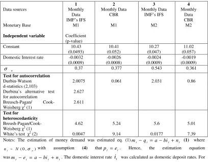
4.3.3 General description of the estimate procedure.

In order to reckon the probability of the collapse of the fixed exchange rate, the estimating procedure was divided into two parts. Firstly, the calculation of the value of parameters will be made such as parameters of money demand

functions: a, b and σn eq. (1) with assumption (4) thatpt =et, the parameters in

the money forecasting rule: and 2 eq. (17), and the variance of the changes in

the foreign interest rate (Appendix B Table 2). The computation of the parameters

of monetary demand (eq. 10) required that it was sensible to use instrumental

variables to eliminate the potential endogenous effect of the domestic interest rate. According to CVW’s paper, there were two instrumental variables: foreign

interest rates (eq. 3) and constant. (see CVW (1989:121)). The residuals from the

monetary demand equations were investigated to examine the phenomenon of autocorrelation or heteroscedasticity between them. For instance, in CVW’s model, they examine the hypothesis of autocorrelation by using tests based on MA(n) process. In this model the process AR(n) was investigated instead of

MA(n).The reason is that MA(n) can be converted to the AR(n) and MA(n) as the

finished process of AR(n). The hypothesis of autocorrelation was estimated by using the test based on AR(n) process. Then an assumption (3) in the theoretical

model (eq. (3)) was analyzed by using the Dickey- Fuller test. If the null

hypothesis is rejected, this means that the foreign interest rate followed a random

path (Appendix B Table 3): it =it− +ut

* 1 *

where ut ~N(0,

σ

Lastly, the parameter of the forecasting rule for domestic credit growth was calculated. CVW simplified the calculation by introducing the definition of

1 +

t

of period t+1. υt₊₁ is from gt+1=Egt+1+υt+1 (26), and with the forecasting rule for

domestic credit growth (17), they obtained E_tg_t+1 =λ∗E_t−1g_t +(1−λ)∗g_t(27).

The first part of equation (27) λ∗Et−1gtcame from the formation of rules

of expectation where past expectation formation has an impact on future

expectation. The second part (1−λ)∗gt comes from the eq. (17) when i=0.

From eq. (27) and (26) they derived: gt+1 −gt = υt+1 −λ∗υt(28).

By assuming that all information is available to market investors and

market agents are rational, they calculated the forecast for domestic credit realisation which contained past forecast errors, so all one-period-ahead forecast

errors are uncorrelated. In accordance with eq. (28) the variance and first

auto-covariance of the first difference in the growth rate of domestic credit was

calculated: g_t+1−g_t as ₍₁ 2₎ 2

υ

σ λ

− and 2

υ

λσ

− , respectively. However, the variance

formula was different compare to CVW’s model (Appendix B-12). By using the sample estimates of variance and the auto-covariance of the first difference in

domestic credit, I computed the λ by using the combination of these formulae.

When I obtained all the necessary parameters to calculate gˆ_t+1 in eq. (22),

I could derive the formula for gˆ_t+1 by transformations of eq.(22) which depended

only on the unknown R. Then, by using this formula, I computed the integer of

eq. (25) with respect to the level of foreign reserve and in that way, obtained the

probability of the collapse of the fixed exchange rate.

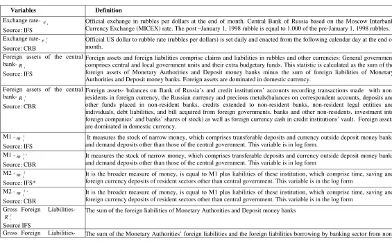
4.4. The data and explanatory variables

domestic credit, foreign capital shocks. The description of the specific data series

used for the calculations is in Appendix C Table 1. In my analysis, two different

data sources were implemented in this analysis: IMF statistics (IFS- International Financial Statistics) and the Monthly Bulletin of the Central Bank of Russia

(Central Bank of Russia: Monthly Bulletin). Since both datasets have their strengths and weaknesses, both were used in my empirical analysis in order to check the robustness of the results. My model consisted of monthly observations from December 1995, to December 1998. The choice of this period was due to it being one of the most stable in political and economic terms - after the establishment of the autonomy of the Central Russian Bank, incorporating the disinflation program, and several official confiscations of population cash

holdings in January 1991, July 1993(see Appendix A Table 1 and section 3.1).

Unfortunately, the monetary base in the Russian case was no recorded in this date. Approximations were implemented - M1 and M2. As a result, the method of calculation in comparison with CVW (1989)’s paper was changed. Moreover, data from the consolidation balance sheet of the banking system (the monetary authorities -central bank- plus the commercial banks) was implemented.

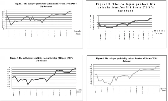
4.5. Empirical implementation and results

data sources (IFS and CBR). Because of that four sets of probability result were analysed (Appendix C Figure 1-4).

All the estimates for money demand looked reasonable (Appendix C Table1), the sign and size of parameters were consistent with economy theory and the empirical analysis of money demand (Gerlach-Kristen (2001:55-554)). However, for the IFS data, there was the problem of heteroshedasticity, but an examination of the residuals did not show any problem with the autocorrelation (Appendix C: Table 1). To reduce the problem of heteroshedasciticy, White’s

matrix was used. In estimating the base money demand parameters in equation (1)

with assumption (4) any technique with instrumental variables were not employed

due to the Hausman –Wu tests for the two instruments (constant term and foreign interest rate) and one instrument (foreign interest rate) rejected the null hypothesis. In the case of the IFS data, it seemed that it did not have to take account of potential endogeneity problems.

On the other hand, these estimates of the CBR data (Appendix C: Table 1) suggest some problems with autocorrelation and heteroshedasticity. Firstly, the instrumental variables were implemented because of a potential endogeneity problem. A wrong sign for the coefficient before the interest rate was obtained. This suggests that there is problem with the omitted variables such as income or approximations of inflation, or there is a problem with the default risk. However, to obtain a more detailed picture of the Russian crisis and to simplify the analysis, the assumption was implemented that these results are as good as the results from using the IFS data. In addition, the residuals from the money demand function

were calculated so that assumption nt ~ N(0,σn)in eq. (1) is correct.

these tests is that although the null hypothesis was originally derived for an AR(p) process (for Durbin-Watson test it is AR(1)), these tests are powerful against MA(p) processes as well. Due to this serendipitous result, the MA(p) and AR(p) are locally equivalent alternatives under the null hypothesis. The only problem

was heteroscedasticity, but the correlation using White’s matrix allows the

assumption about the residual from the money demand equationnt ~N(0,σn) to

be upheld.

The next step was to investigate the assumption about the random path of interest rates. The modified Dickey-fuller t test proposed by Graham, Rothenberg, and Stock (1996) was implemented. This Dickey-Fuller unit root test allowed

finding that the coefficient of *

1

−

t

i is equal to one (the null hypothesis: it is not a

static process). The null hypothesis of the unit root in the foreign interest rate is not rejected at a reasonably significant level of 5 percentages, the same extent at which the foreign interest rate is assumed to be correct (Appendix C, Table 2). Additionally, both tests of autocorrelation for the first difference of i* were also carried out and yielded no evidence of autocorrelation.

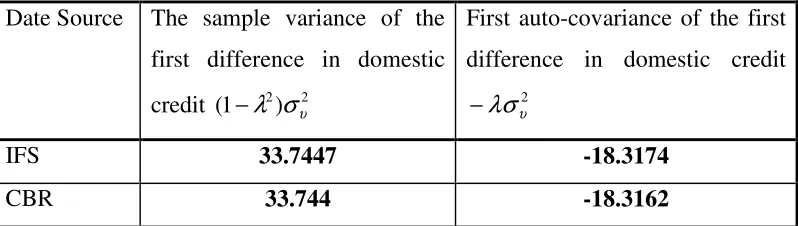
The last thing before computing the integral of eq. (25), was the

computation of . Using the sample estimate of variance and the first

auto-covariance of the first difference in domestic credit (Table 1) obtained λ=

0.43946 for IFS data and respectively for CBR data λ= 0.43845. In order to

simplify all the calculations, one value of λ= 0.44 for both sets of data was

used.10

10 _{The root of the quadratic was chosen that is less than one in absolute value in order to insure}

Table 1

Date Source The sample variance of the first difference in domestic

credit ₍₁ 2₎ 2

υ

σ λ

−

First auto-covariance of the first difference in domestic credit

2

υ

λσ

−

IFS 33.7447 -18.3174

CBR 33.744 -18.3162

Source: My own calculations based on Table 2 and 3 from Appendix C.

The series of one-step devaluation probabilities for the Russian fixed exchange rate was calculated in the followed way. In estimating the collapse probabilities, the equation was solved by substituting the parameter estimates above and the data associated with each observation for four different sets of data to obtain an estimate of the critical values for domestic credit growth in each

period. The residuals parameters were ignored, which appeared in eq. (22)

because this residual behaviour is treated as white noise. Then eq. (25) was

integrated to get the probability. As this integration from eq. (25) could only be

computed by using the numerical integration, CVW used the Simpson’s rule- the

trapezoidal rule. In this paper eq.(25) was also computed by using the trapezoidal

rule (Appendix B-13).

The probability estimates (Appendix C: Figure 1-4) look quite reasonable,

both in the estimated magnitude of the probability (interval 0-1) and in their behaviour over time (Appendix A, Chapter 3.1) Estimates for the collapse probability were also found, along with domestic credit growth (cumulative

growth since the end of 1995) (Appendix C: Figure 1-4). These tables suggest that

the permanent increase in domestic credit growth brought about the loss of

words, the credibility of the policy for a fixed exchange rate was undermined even when the authorities said that the fiscal and domestic credit policies were consistent with the exchange rate. In addition, these results also indicate that confidence was never fully restored and that just prior to the collapse of the fixed

exchange rate in 1998, the credibility of the fixed exchange regime was extremely low. The estimated probability was quite high through all the period except at the beginning and middle of 1996. During this period there was a strong disturbance in the probability, which could have been caused by changes in the fiscal and monetary policy (changes in the exchange corridor between January and June)( Buchs (1999:694-696)). In the middle of 1997, domestic credit growth exceeded 50 percent (according to IFS data, and 29 percent in CBR data) and the collapse probability started to permanently increase. The cumulative point was at the end of 1998, when 78 percent (according to IFS, and 65 percent in CBR data) expansion in domestic credit growth undermined the credibility of the announced fixed exchange rate mechanism and the collapse probability rose above 90 percent in August 1998, for all four figures. To the same extent, the empirical findings suggest that the probability associated with regime changes in August 1998 was mainly attributable to the speculative pressure in the light of deterioration in economic fundamentals (the first generation model). In line with expectations, the probability of devaluation was found to be in the increased levels of central bank credit to the banking system. The increase fiscal deficit and the reduction in foreign exchange reserves were also linked to the probability of devaluation.

5. Implication of IMF’s intervention

effect was in the short term. However, it can illustrate the issue about the importance of the IMF program. Throughout the 1990s, Russia operated under the auspices and close scrutiny of a Fund (support and stabilisation program). Another question is how it could happen that the IMF did not recognise that

Russia was almost typical of a first generation crisis through some aspect of other generation models (Chapter 4.1. and 4.5).

At the beginning of the 1990s, Russia was under ‘shock therapy’, which was strongly promoted by IMF advisors. According to this plan, it was reasonable to remove the central plan with the decentralisation market system, and secondly, to replace public ownership with private property, and eliminate or at least reduce the distortions by the liberalisation of trade. To the same extent, liberalisation and stabilisation were two of the pillars of the radical reforms strategy. The rapid privatisation was the third pillar. In addition, the IMF supported international loans to Russia (Stiglitz (2002:136-140)). The SDR loaned 2.8 billion dollars since 1992 up to 1994 but, as the first tranche of loans, they did not carry mandatory programs. Then, after the economic problem in 1994, the IMF gave

standby credit of $ 6.8 billion to improve the reforms of the monetary policy and improve fiscal policy tightness. However, the IMF did not even suggest using the exchange rate as an anchor; it merely supported the Russian decision to adopt the ‘corridor’, the crawling peg. The IMF’s second large-scale program came in the run up to 1996 election. However, the conditions after the reforms were quite vague and, as matters grew worse, the government did not seem to realise the seriousness of the situation. It concentrated its efforts on improving the budget, with no positive results. A new program was agreed upon in July 1998 when the crisis was already under way (Ivanovo and Wyplosz (2000:4)). The government’s

publicly stated strategy, the July Package, contained three main elements: a