Munich Personal RePEc Archive
Combining Energy Networks
Abrell, Jan and Weigt, Hannes
Dresden University of Technology
February 2010
Online at
https://mpra.ub.uni-muenchen.de/65504/
E
lectricity Markets Working Papers
WP-EM-38
Combining Energy Networks
Jan Abrell and Hannes Weigt
February 2010
Dresden University of Technology Chair for Energy Economics and
Combining Energy Networks
Jan Abrell and Hannes Weigt
Corresponding author: Hannes Weigt
Dresden University of Technology Faculty of Business and Economics
Chair of Energy Economics and Public Sector Management 01069 Dresden, Germany
Phone: +49-(0)351-463-39764 Fax: +49-(0)351-463-39763 [email protected]
Abstract:
Electricity markets rely on other upstream energy markets like oil, gas, and coal to provide the necessary fuel for generation. As both the electricity market and those upstream markets rely on networks, congestion on one market may lead to changes on another. In this paper we analyze the interaction of the natural gas network with the electricity network applying a partial equilibrium approach. The model is applied to a stylized representation of the European energy markets. We apply the model to two cases: first the impact of a supply reduction of natural gas on both markets by cutting imports from Russia, and second, the impact of the introduction of an emission restriction on electricity generation. Since natural gas can be an input for electricity generation, gas price level changes alter the generation dispatch. However, the network character of both markets leads to further effects that are not obvious on first sight. Congestion between markets and particular effects due to loop flows in electricity markets can lead to price and quantity effects in markets far away from the initial cause of market changes.
1
Introduction
Within the next decades, energy markets around the world face a multitude of challenges. Markets formerly characterized by imperfect competition are in the process of being restructured to competitive industries. Carbon emissions need to be reduced for a sustainable future. Long term investments need to be stimulated in order to guarantee security of supply of energy commodities. Already challenging tasks in isolated markets, the interaction of energy markets further complicates these processes. Electricity markets serve as a linkage between different fuel markets as in the long run fuels can substitute one another. Consequently, decisions regarding the future development on electricity markets such as the projected ENTSO-E Ten-Year Network Development Plan will have a direct impact on the upstream fuel markets. Likewise, the imposition of carbon regulation favors the use of less carbon intensive fuels and, in turn, stipulates demand for these fuels. On the other hand, market or investment decisions on fuel markets – such as the projected increase in LNG import capacities in Europe – have a direct impact on the downstream electricity market as they influence the availability of fuels and change the price levels. This interaction is further complicated by the fact that most fuel markets rely on some kind of network infrastructure (pipeline, sea routes, and railways) to distribute their commodity. Similarly, electricity markets are grid-bounded and have to take account of physical power flow laws. The different networks are characterized by a substitution relationship. For example, electricity can be produced and sold in Germany using a gas-fired power plant requiring pipeline transport of the natural gas to Germany. Likewise, electricity can be produced in the Netherlands and sold in Germany using the electricity grid. However, this substitution is bounded by the capacity of the transmission grid. Therefore, congestion effects typical for grid-bounded transportation need to be taken into account when analyzing the interaction of energy markets and the energy system as a whole.
The objective of this paper is to provide a modeling framework that accounts for the interaction of fuel and electricity markets while simultaneously respecting the network character of those markets. We apply the framework to a stylized representation of the European market. Simulating a short-fall of Russian natural gas exports and an emission reduction requirement, the results illustrate the importance of network representations analyzing energy markets. The interaction highlights the importance of a combined market assessment. Particularly, with respect to the aim of an internal fully liberalized European energy market impacts along the market chain need to be taken into account when deciding about future regulation, investment or market design plans.
Concerning energy markets, two facts are important to recognize: First, energy markets are highly connected by electricity generation which relies on coal, natural gas, and oil as production input. Second, energy commodities such as electricity and natural gas are characterized by grid-bounded transportation. In turn, this has led to two different streams of numerical modeling approaches.
demands. However, these models tend to simplify transmission modeling by abstracting from networks such as natural gas pipelines or electricity grids. In a partial equilibrium setting, such models are formulated in an optimization framework such as e.g. MARKAL (Loulou et al., 2004 ), POLES (Kouvaritakis et al., 2000), MESSAGE (Grübler and Messner, 1998), or in an equilibrium format such as LIBEMOD (Aune et al. 2001). More macroeconomic oriented models with a focus on the representation of the energy system are represented either in a computable general equilibrium format such as e.g. the MIT-EPPA (Paltsev et al., 2005) and GEM-E3 (Capros et al., 1997) model or as intertemporal welfare maximizing Ramsey-type models e.g. REMIND (Bauer et al., 2008) On a more technical oriented level simulation and optimization approaches are used. These models are often focused on material flows, the optimal fuel usage, or power plant mix. In this class, the PERSEUS-EEM model is close to our work (Möst and Perlwitz, 2009). They include a natural gas pipeline into a cost minimizing inter-regional long-term model. In contrast to our work, the approximate electricity transport by net-transfer capacities, i.e. do not explicitly model loop-flows typical for electricity grids. On the other hand, a broad stream of literature analyzes single energy industries with a detailed representation of the technological details of grid-bounded transmission. As grid-bounded transmission leads to natural monopolies such model particularly emphasize the role of imperfect competition. Mathiessen et al. (1987) show that the European natural gas market is best described by a Cournot duopoly. Gabriel et al. (2005) and Egging et al. (2009) presented a Nash-Cournot framework of the US and European natural gas market including pipeline and Liquefied Natural Gas (LNG) transportation. EWI Cologne has produced a series of linear optimization models of which the TIGER model provides the most detailed dispatch model for Europe and is suited for identifying congestion (Perner and Seeliger, 2004; Lochner and Bothe, 2007). Holz (2009) discusses these different model families in more detail.
Network oriented electricity market models include the power flow along different lines. In contrast to natural gas pipelines, in an electricity network the power flow is physically determined by the injections and withdrawals at nodes, i.e. loop-flows need to be modeled. Smeers (1997) and Ventosa et al. (2005) provide an overview over numerical modeling approaches. As natural gas models, network oriented electricity models examine the effect of imperfect competition (e.g. Hobbs, 2001; Neuhoff et al., 2005). Furthermore, network models applying the DC load flow approach are commonly used for economic market analyses (e.g. Stigler and Todem, 2005; Green, 2007; Leuthold et al. 2008).
natural gas flows.1 The approach has been extended by e.g. Unisihuay et al. (2007) for multiple interconnection points. Arnold et al. (2008) present a decomposition approach for the GEOPF in order to allow larger dimension applications. While the GEOPF approach represents technological details in great detail, it is limited from an economic point of view as the usage of integer variables leads to problems representing price variables (O’Neil et al., 2005).
In this paper, we present a general framework to combine energy markets including detailed network characteristics using the mixed complementarity problem format. Concentrating on the natural gas transmission stage, i.e. assuming directed pipeline flows but avoiding integer modeling problems, our approach allows for a more detailed analysis of energy systems on a large regional scale. Similar, focusing on electricity transmission, we derive a power flow based market representation applying the DC load flow approach. In a stylized model of the European energy market, we present two scenarios – the reduction of natural gas imports from Russia and the imposition of a carbon emission constraint on the European electricity sectors – which highlight the importance of recognizing the economic interaction of grid-bounded energy commodity transport.
The remainder of this paper is structured as follows. Section 2 describes the modeling framework. First, the single market models are presented. Afterwards, the combination of the single market model is described. In Section 3, we parameterize the modeling framework to the European Union, describe the scenarios and present their results. Finally, we summarize our work, draw conclusions, and identify fields for future research.
2
Model Description
Following we will formulate the market representations for the electricity, the natural gas and the combined setting. The models will be defined as Mixed Complementarity Problem (MCP) (e.g. Rutherford, 1995);
(1)
n nn
T
given f : find r
s.t. r 0 f r 0 r f r 0
Following Mathiesen (1985) two types of equilibrium conditions can be distinguished in an MCP: zero-profit and market clearing conditions. In general, zero-profit conditions are complementary to activity variables, while market clearing conditions are associated with prices.
The considered markets differ in their network representation but have similarities in the definition of producers and consumers. Producers are assumed to maximize their profit given technical constraints whereas consumer behavior is defined via a demand function. Each producer is endowed with production capacity with specific unit cost. Network operation is assumed to be managed by a single network operator also acting as the market operator clearing production and demand.
1 Put differently, at the distribution stage pipeline flow are undirected. Thus, the decision using compressors results in a
2.1 The natural gas market
Natural gas is either transported via pipelines or using liquefied natural gas (LNG) tankers. In both alternatives, the operator has full control of the amount injected into the network and the routes chosen to transport the gas. However, while in pipeline networks the capacity of a pipeline is restricted, LNG flows are restricted by the liquefaction and regasification at the origin and destination nodes.
We denote nodes in the natural gas network by g and h Є G. A node is characterized by the supplier at
these node, natural gas demand, and the liquefied natural gas (LNG) technologies, i.e. the liquefaction regasification potential. Nodes are connected via pipelines of a given capacity capg,hpipe. LNG
connections between nodes are unrestricted in capacity but restricted by the available liquefaction (capgliq) and regasification (capgreg) capacities.
Five market participants interact in the model: Natural gas producers, traders, the pipeline operator, LNG operators, and final consumers. Final consumers are served by traders only. Producers extract the natural gas and sell it either to the trader or to the LNG operator. The LNG operator buys the natural gas from producers at some node (with liquefaction capacity), transports it to another node (with regasification capacity), and sells it to the trader. Traders buy natural gas from producers or LNG operators, buy the transport service to transport the gas from the pipeline operator, and sell it to the final consumers. The pipeline owner operates the pipeline network and rents out capacity to the trader in order to transport natural gas.
Final consumers are represented by a linear demand curve:
(2)
0
gas gas gas gas gas
g g g g g
DEM a b PD DEM
Where DEMggas and PDggas are natural gas demand and price at node g. aggas (bggas) are strictly
positive (non-positive) constants.
Constant extraction costs cggas and the extraction capacity capggas characterize the natural gas producer
at node g. Assuming perfect competition, each producer maximizes his profit under the extraction
capacity restriction choosing the extraction quantity Xggas given the natural gas supply price PSggas:
0
max
gas ggas gas gas
g g g
X
PS
c
X
s t
. .
capggas Xggas PCggas 0 (3)PCggas is the scarcity price of the extraction capacity at node g. Accordingly, the zero-profit condition
for each producer becomes:
(4)
0
gas gas gas gas
g g g g
c PC PS X
The LNG trader buys natural gas at node g from the producers at the supply price and sells it at node h
also at the supply price to traders. LNG transport on a specific route from g to h incurs constant units cost cg,hLNG. Furthermore, the liquefaction and regasification process require energy in form of natural
constraint choosing the transported volume Tg,hLNG (i.e. the volume net of liquefaction losses but gross
of regasification losses) given prices:
, , , ,
max
LNG g h gas ggas LNG LNG
h g h
T g h
PS
PS
c
T
g h
s.t. reg LNG,
reg
0
g h g g
h
cap
T
PC
(5)(6)
,
0
liq LNG liq
g g h g
h
cap
T
PC
PCgliqand PCgreg are the scarcity prices of liquefaction and regasification capacity, respectively. The
corresponding zero profit condition for the transported LNG volume becomes:
,
,
0
gas g
LNG liq reg gas LNG
g h g h h g h
PS
c
PC
PC
PS
T
(7)The trader buys natural gas at node (
g
Tgbuy) and sells this gas at node h (Tg hgas, ).2 In order to transportthe gas from node along the pipeline from
g
g to h ( gas, , g g hF ) he has to buy transport service from the pipeline operator at price PTg,hpipe. Therefore, the trader maximizes his profit by choosing the
purchased and sold amount of natural gas and the flow along the pipelines under the flow conservation constraint for each node:
, , ,
, ,
,
max
, 0 , ,buy gas gas g g h g g h
, ,
gas gas gas buy pipe gas h g h g g g h g g h T T F
g h g g h
PD T
PS
T
PT
F
s.t. gas, ,
buy gas, , gas, gas, free (8)g g h g if g h g h g g h g h
g g
F T F T PN
, gas g hPN is the nodal price of the gas bought at node g at node h. The corresponding zero-profit
conditions for the purchased and sold amount and the pipeline flow are given as:
(9)
, 0
gas gas gas
g h h g h
PN PD T,
(10)
, 0
gas gas buy
g g g g
PS PN T
(11)
, , , , , 0
pipe gas gas gas
g h g g g h g g h
PT PN PN F
The pipeline operator maximizes his revenues under the pipeline capacity constraints choosing the total flow of natural gas along the pipeline connecting g and h (Fg,hpipe ):
, , , , 0 , max gas g hpipe pipe pipe g h g h g h F g h
PT c F
s.t. pipe, pipe, pipe, 0 (12)
g h g h g h
cap F PC
PCg,hpipe is the scarcity price of pipeline capacity. The zero-profit condition for the optimal flow along
the pipelines results as:
g
(13)
, , , , 0
pipe pipe pipe pipe
g h g h g h g h
c PC PT F
Prices are determined by market clearing conditions. At the supply market, the total available quantity is determined by production and the amount shipped to that node. Demand consists of purchases by the trader and LNG shipped away from this node (including liquefaction losses):
,
,
0
LNG g h
gas LNG buy gas
g h g g g
h h
T
X
T
T
PS
(14)
At the demand market the trader offers natural gas to final consumers:
(15)
,
0
gas gas gas
h g g g
h
T
DEM
PD
The market clearing condition for pipeline flows determine the transport price along a given pipeline:
(16)
, , ,
,
0
pipe gas pipe
g h g g h g h
g
F
F
PT
The full natural gas model consists of equation (2) to (16).
We note that we have stated the model without defining a set of pipelines, possible natural gas origin or destination nodes, or LNG trading routes. Numerically implementing the model, we construct these sets out of the capacity parameters and fix variables for which no capacity exists to zero in order to reduce the size of the model.
The model is static. Therefore, we decided not to include natural gas storage facilities. However, extending the model to include storage can be done by adding the zero-profit condition of the storage operator and the respective demand and supply to the market clearing equation (14) and (15). Assuming constant unit costs for all market participants and linear demand, we developed the model as a linear complementarity model. The restriction of linearity can be relaxed by putting other demand function into equation (2) and replacing the constant unit costs by some marginal cost function. The presented pipeline network consists of arcs with exogenously given direction using the pipeline capacities. Finally, we assumed perfect competition at all markets and, accordingly, representative agents. While relaxing this assumption for one group of market participants under simultaneous model timing is possible, introducing sequential timing is difficult resulting in mathematical or equilibrium problems with equilibrium constraints (M/EPEC).
2.2 The electricity market
Contrary to flows in the natural gas network, which are under the control of the network operator, system power flows in an electricity network are determined by Kirchhoff’s laws. Thus, injections and withdrawals at nodes impact the whole power flow pattern in the system leading to the problem of loop flows.3 Consequently, the choice variables of the grid operator are the amount of power injected
or withdrawn at different nodes while the flows are solely determined by physical laws.
3 For example, transporting electricity from the North of Germany to the South of Germany also leads to cross border flows
We denote nodes in the electricity network by e Є E. A node is characterized by the generators at these
node and electricity demand. Nodes are connected via lines l of a given capacity caplline. Three market
participants interact in the model: generators, the network operator, and final consumers. Final consumers are served by the network operator, only, and generators sell to the network operator. The electricity network system operator does not trade on specific node pair combinations like in the natural gas setting or even specific lines. The whole power flow pattern is determined once the injections/withdrawals are set. In order to derive a mathematical formulation of this problem we include a hub node which roots all transactions taking place within the network. The system operator transfers all generated energy from the nodes e to the hub node and in turn provides all demanded
energy at the nodes e via deliveries from the hub node. Thus, the choice variable for the system
operator is the amount of energy transported to or from the hub to a node (Ye) which can be positive or
negative depending of the definition of the energy balance (equation 23). The price of transmitting power is denoted as PTe and the system operator is maximizing its profits from transaction to and
from the hub.
Those transactions are mere financial constructs capturing the resulting price divergences due to physical constraints. The system operator has to ensure that the chosen injections and withdrawals at each node do not violate the existing line capacities caplline. In order to derive the power flow pattern
one can use power transmission distribution factors (PTDFle) which state the share of a flow on a
specific line resulting from specific injections/withdrawals. The whole system operator’s problem becomes:
max
eel e e Y
e
PT Y
s.t. line
le e l l
e
PTDF Y
cap
PC
(17)line
le e l l
e
PTDF Y
cap
PC
(18)Equation (17) and (18) secure that the power flow on a line l does not exceed the capacity boundaries of the line caplline. As electricity flows can be positive or negative depending on the flow direction the
capacity restriction has to hold in both directions. PCl+ and PCl- are the corresponding scarcity prices
of line capacity. The zero-profit condition of the system operator is given as:
el
e le l l e
l
PT
PTDF
PC
PC
Y free
(19)The relevant nodal electricity price Peel therefore is divided into two components: first a marginal
energy price defined via the market clearing of the whole system (PHUB) and the transmission fee due
to network congestion (PTe). The price at a node can be derived by summing those two components.
Since PTe can be positive or negative the locational price can diverge in both directions from the Hub
price.
Final consumers are represented by a linear demand curve:
el el el el el
e e e e
Where DEMeel is the electricity demand, PHUB and PTe yield the price at e. aeel (beel) are strictly
positive (non-positive) constants.
Generators at node e are defined by the available generation capacitiesof plant type iЄI (capieel). The
generation costs depend on the exogenously given price of fuel f Є F fuel price pffe and efficiency
level ηfie depending on the plant and fuel type.4 In order to derive carbon emissions, each fuel is
characterized by its physical carbon content θf. Assuming perfect competition, each generator
maximizes his profit under the capacity restriction choosing the generation quantity Xieel given the
electricity price Peel consisting of PHUB and PTe as well as the emission price Peemi:
0 : 0
max
el efie
emi fe f e
el el
e i
X i f
fie
pf
P
PT
PHUB
X
es.t. el el el
0
(21)ie ie ie
cap
X
PC
PCieel is the scarcity price of the generation capacity of plant type i at node e. Accordingly, the
zero-profit condition for each plant becomes:
0 emi
fe f e el el el
e e ie
fie
pf P
PC PT PHUB X
(22)
The transmission prices PTe are determined by the market clearing condition for the system operator.
At any node the energy injected or withdrawn from the grid has to equal the difference between generation and demand:
free
el el el
e ie e e
i
Y
X
DEM
PT
(23)Furthermore the overall market clearing condition defines the system marginal price PHub:
(24)
,
0
el el
ie e
i e e
X
DEM
PHUB
Denoting the exogenously given allowed carbon emissions at node e by Eemax, the carbon price at a
node is determined by the following market clearing condition:5
max
, : 0
0
fieemi
f e el emi
e ie
e f fie
P
E
X
P
e
(25)
The full electricity model consists of equation (17) to (25). Similar to the natural gas model the electricity model is static. Therefore, pump storage facilities are not regarded but could easily be added by including the zero-profit condition of the storage operator and the respective demand and supply to the market clearing equation. Furthermore, we imposed linearity and perfect competition.
4 For the sake of simplicity, we assume that each plant type produces with only one fuel, i.e. for each (
i,e)ηfie is strictly positive for exactly one fuel f. Therefore, the efficiency parameter also serves to establish a mapping between the generation technology set I and the set of fuels f. Relaxing this assumption, requires extending the range of the generation variable, i.e. introducing Xfieel as the amount generated by plant i at node e using fuel f.
5 We formulate the general model with an emission restriction at every node. However, the modification for allowing
2.3 Combining energy networks
In order two combine the models, two steps are necessary: First, we need to determine at which nodes electricity generators demand natural gas, i.e. which nodes of the gas network are also nodes of the electricity network. Second, the models are linked by making the demand in the gas network and the natural gas price in the electricity model endogenous.
For the first step we assume that natural gas is supplied to each electricity generator. However, natural gas is also delivered to non-electricity nodes. We establish a mapping (i.e. a two dimensional tuple) between the set of natural gas and electricity nodes which is denoted as GE(g,e) and associates each
electricity node to exactly one natural gas node. However, one natural gas nodes may serve various electricity nodes. At the electricity generation nodes, natural gas demand consists of the demand of electricity generators and further residential demand. Accordingly, generators’ demand is added to the natural gas demand market clearing equation (15). Denoting the natural gas plant as gas Є I and
natural gas as fuel also by gas Є F, the natural gas demand market clearing equation at electricity
generation nodes becomes:
, , ( , ) , , 0 el gas e
gas gas gas
h g g g
h e GE g e gas gas e
X
T DEM PD g N
(26)We now endogenize the natural gas price in the electricity model. This is done by replacing the generators’ zero profit condition (22) by a version with the natural gas price as a variable. For natural gas plants the equation becomes:6
( , ) , , , 0 gas emig i e
g GE g e el el el
e e i e
gas i e
PD P
PC PT PHUB X i gas
(27)For non-natural gas plants, the generators’ zero profit condition remains the same:
0 \ emi
fe f e el el el
e e ie
fie
pf P
PC PT PHUB X i I gas
(28)The combined model consists of equation (2) to (28) without equation (15) and (22). Obviously, the underlying assumptions are the same as those in the single models.
3
Sample application
3.1 Parameterization and scenarios
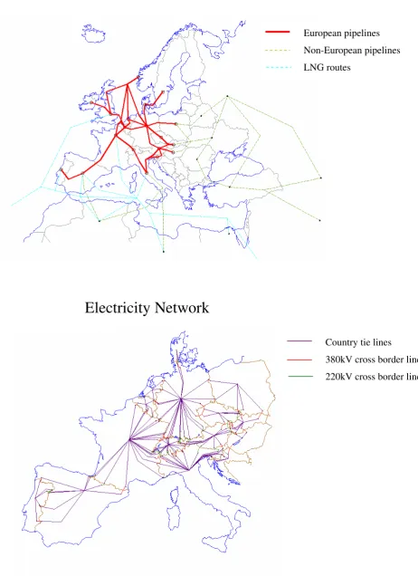
In our application, we combine a stylized representation of the European natural gas and electricity transmission markets. The basic model parameters are taken from Neumann et al. (2009) for the gas market representation and from Leuthold et al. (2008) for the electricity market. The combined model covers central and western European countries with respect to natural gas and electricity demand
6 Note that by the above assumption that each electricity node is served by exactly one natural gas node, the sum on the left
(Figure 1). Whereas the gas model also includes the UK, Ireland, Norway and Sweden as demand nodes and several exporting nodes outside Europe (e.g., Russia, Algeria, and Lybia), the electricity market representation is limited to the continental European countries. Both markets are represented in a highly stylized setting with one node representing the whole country. Cross border transmission is either modeled by single connections between those country nodes (natural gas) or via several cross border lines connected to the respective country nodes via tie lines (electricity).
The model is calibrated to represent 2005 values (see Table 4 in the Appendix). The time resolution of the model is limited to an average hour not taking account of seasonal or daily demand and production patterns. Natural gas and electricity demand are taken from Eurostat (2010). Demand is assumed to be linear based on reference demand and price values with an elasticity at this reference point of -0.5 for natural gas and -0.25 for electricity. Electricity generation is clustered into nine technologies based on UCTE (2007): nuclear, lignite, coal, gas, oil, mixed, other, hydro, and pumped storage.7 Table 1
shows the underlying assumptions regarding fuel prices, efficiency and emission factors. We do not account for spatial differences in those values.
We analyze three different scenarios to highlight the interaction between the linked markets. First a
Base case is derived applying the above described dataset. This base case represents the benchmark of
our analysis. In the second scenario we analyze the impact of a change in the natural gas market on the system (Russian case). We assume a sharp reduction in exports from Russia via the Ukraine to a level
of about 50% of the base case exports. This will lead to supply shortages in South-East Europe, impact the natural gas flow and price pattern and, thus, possibly the electricity generation. In a third scenario we analyze the reverse interaction due to a change in the electricity market setting by introducing emission trading (Emission case). Taking the base case emissions as benchmark we require a 15%
[image:13.595.80.390.555.699.2]emission reduction target. The resulting emission allowance price will lead to a reduction of the cost advantage of coal in favor of natural gas which increases the demand for the latter which impacts the natural gas market.
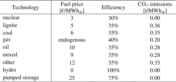
Table 1: Electricity generation specifications
Technology [€/MWhFuel price
th] Efficiency
CO2 emissions
[t/MWhth]
nuclear 3 30% 0.00
lignite 5 35% 0.36
coal 6 35% 0.35
gas endogenous 40% 0.20
oil 10 35% 0.28
mixed 9 35% 0.28
other 12 35% 0.35
hydro 0 100% 0.00
pumped storage 25 75% 0.00
Source: IPCC (2006), own assumptions
7 Mixed generation represents a large variety of multi fuel engines running on coal and/or gas and/or oil. We do not consider
Figure 1: Networks
Natural Gas Network
Electricity Network
Source: based on Neumann et al. (2009) and Leuthold et al. (2008)
European pipelines Non-European pipelines LNG routes
3.2 Result overview8
In the Base case the natural gas market can roughly be clustered into three supply regions: Western
and Central Europe are largely supplied with natural gas from the North Sea (Norway and the Netherlands), Eastern Europe is supplied by Russia, and Southern Europe is supplied by Africa (Algeria and Lybia). The Iberian Peninsula does not exchange gas with the rest of Europe and is solely relying on African gas and LNG import. Italy is, beside the African amounts, importing gas via its northern neighbors Switzerland and Austria. A similar pattern can be observed in the electricity market. Spain and Portugal are a separate price zone due to congestion between France and Spain (Table 2). Italy is the “electricity sink” of Europe which consequently leads to a high price level and congestion at the cross border lines. Northern and Eastern Europe are more or less on a coal based price level. The generation pattern follows the merit order with hydro, nuclear, and lignite being fully utilized (Table 3). Coal and gas power plants are dispatched according to the availability capacities within the country taking into account the local natural gas price (cost parity of electricity from gas and coal occurs at a gas price of 6.85 €/MWh).
In the Russian case the imports via the Ukraine are significantly reduced which leads to higher natural
gas prices in South East Europe (Table 2). Furthermore, Italy faces higher prices and routes a part of its African imports to Austria and Slovenia. The situation in North and West Europe is similar to the
Base case as neither the North Sea gas nor the Russian imports via Belarus and Poland are affected. In
the electricity market those countries facing higher gas prices in general also face higher electricity prices. In contrast the Benelux and France face slightly lower electricity prices (Table 2). The generation dispatch for hydro, nuclear, and lignite is similar to the base case as those technologies are cheaper than coal or gas and dispatched according to the merit order. Electricity generation from natural gas drops to 27 GW (from 40 GW in the base case) due to reduced output in Italy and Hungary. Overall coal generation remains at a level of about 50 GW (Table 3).
In the Emission case the allowed total emissions are cut to 85% of the emissions in the base case. Due
to the binding emission cap an allowance price of about 5.5 €/tCO2 occurs and consequently electricity
prices increase on average (Table 2). As coal units emit about 1 t per generated MWh electricity whereas natural gas units only emit 0.5 t the price parity between coal and gas is now at a natural gas price of 7.86 €/MWh. Consequently gas based electricity production is increased to about 50 GW while coal is reduced to 30 GW (Table 3). This leads to a general increase in demand for natural gas and on average to higher domestic gas prices across Europe even in countries that do not increase gas based electricity generation like (Benelux) or that are not accounted for in the electricity model (UK). In contrast, Portugal and Spain even face a gas price decrease (Table 2).
As LNG capacities are already binding in the base case, none of the scenarios affect LNG trade
patterns.
Table 2: Demand price outcomes [€/MWh]
Base case Russian case Emission case
Country Natural gas Electricity Natural gas Electricity Natural gas Electricity Austria 8.46 18.86 11.26 19.32 8.46 24.17
Belgium 8.40 18.91 8.42 18.23 8.73 23.34
Czech Republic 8.29 17.35 8.31 17.40 8.46 23.33
Denmark 6.64 17.14 6.66 17.14 6.97 23.21
France 8.95 16.21 8.97 15.98 9.28 17.39
Germany 7.74 17.14 7.76 17.14 8.07 23.21
Hungary 8.34 20.84 10.05 21.63 8.92 25.33 Ireland 8.40 8.42 8.73 Italy 9.78 24.44 10.29 25.71 9.78 27.47 Netherlands 7.08 18.14 7.10 17.76 7.41 23.28 Norway 5.76 5.78 6.09
Poland 6.24 17.14 6.24 17.14 6.24 23.21
Portugal 9.27 23.18 9.27 23.18 8.46 24.19 Slovakia 7.69 16.88 10.49 16.81 7.69 23.06 Slovenia 9.12 11.50 9.12
Spain 9.27 23.18 9.27 23.18 8.46 24.19
Sweden 7.74 7.76 8.07 Switzerland 9.01 14.75 9.52 15.05 9.01 24.33
UK 7.74 7.76 8.07
Table 3: Electricity generation [MW]
Hydro Nuclear Lignite Coal Gas Mixed
Base Case
Germany 2335 18270 18270 17857 0
Benelux 47 5603 0 3968 14712
France 9585 56970 0 0 0
Eastern Europe 1352 7106 15861 14239 2554
Alps 10554 2880 0 1573 90
Italy 6075 0 0 4230 16931
Iberia 7876 6712 3082 8418 5468
Russian Case
Germany 2335 18270 18270 21864 0
Benelux 47 5603 0 3968 14510
France 9585 56970 0 0 0
Eastern Europe 1352 7106 15861 11274 668
Alps 10554 2880 0 1573 90
Italy 6075 0 0 4230 5193 12108
Iberia 7876 6712 3082 8418 5468
Emission Case
Germany 2335 18270 18270 2861 5640
Benelux 47 5603 0 3968 14712
France 9585 56970 0 0 0
Eastern Europe 1352 7106 15861 11795 3457
Alps 10554 2880 0 1573 197
Italy 6075 0 0 4230 15618
[image:16.595.79.538.268.703.2]3.3 Comparison and discussion
Comparing the Russian and the Base case we observe the impact of changes in the natural gas market on the downstream electricity market. The cut of imports from Russia via the southern route including Ukraine, Hungary and Slovakia leads to significant price increases in these countries. Hungary has to completely cut gas based electricity production. Italy also has to sharply reduce its gas based generation since a large fraction of its gas imports came from Russia via Austria. Consequently, more costly mixed based generation is used in Austria. Beside these obvious results which would also be forecasted without a combined model setting several side effects can be observed. Hungary shifts from an electricity export to an import position. In turn, the whole electricity flow pattern in East Europe is affected. To replace the reduced gas generation in Hungary the cheapest alternative is coal energy from northern countries. However, Polish coal generation, although possible from a generation capacity point of view, can not be utilized due to congestion problems between Hungary and Slovakia. Therefore, Germany increases its coal generation to cover the Hungarian demand. However, this changes the power flow pattern via Austria towards Italy. As a result Germany increases its coal production beyond the need of Hungary. In turn, Poland reduces its generation to allow a further power flow towards the import depended Italy.9 A side effect of the increased coal generation in
Germany is the reduced imports via the Netherlands. Therefore, the available Dutch natural gas generation capacities can be slightly shifted to satisfy a larger fraction of the Belgian demand and relive congestion at the Benelux borders. Consequently the price level in the Benelux slightly drops (Table 2).
The emission case illustrates the impact of a change in the electricity market on the upstream natural
gas market. By introducing a binding emission target, the relative marginal cost ratios are altered towards less emission intensive generation technologies. Therefore, a switch from the most emission intensive coal technology to the least intensive gas technology is observed. Due their non-emitting character and since they are already at the capacity bound in the base case, hydro and nuclear based
generation does not alter. Furthermore, as the reduction of coal based generation is sufficient to comply with the reduction target, lignite based generation is also not affected. Coal production is cut back in those countries that are able to compensate the fallback by increased imports or a switch to gas based production. The majority of reduction takes place in Germany were about 15 GW or coal generation is shut down, followed by Poland with about 2 GW. As the carbon price increases the cost of electricity generation, the electricity price increases. In the consequence, demand is decreasing by about 5%. Therefore, the 5 GW increase of gas based generation does not outweigh the decrease in coal based generation. Germany significantly increases its imports which in turn leads to a shift of power flow patterns towards Germany. The only country reducing gas based generation is Italy due to its high gas prices and the electricity demand reduction resulting from the emission allowance price.
9 Coal prices and power plant efficiencies are not locational differentiated. Thus the only cost difference between Polish and
Domestic natural gas prices increase in most countries by 4% to 7%, even in those countries that are not part of the electricity market representation. However, most East European countries do not face a price increase as they are either capable to increase their imports from Russia (Slovakia and Czech Republic) or do not rely on natural gas generation (Poland).
Surprisingly, the Iberian Peninsula even has lower natural gas prices. This is a result of their isolated network situation. Their electricity imports from France are bounded by the low capacities in the Pyrenees and their gas imports by their LNG terminals and connection to Africa. Thus, the introduction of emission trading does not influence the trade pattern in either market. However, the electricity price increase leads to a slight reduction of electricity demand. As the emission price is not high enough, natural gas fired generation is still the marginal technology in the merit order. Therefore, the output of these plants is reduced. The reduced demand for gas of the electricity sector causes a price decrease which, in turn, stimulates final demand. Therefore, the total gas demand (consisting of domestic and electricity gas demand) does not change in these countries.
Although, the presented results are highly depended on the chosen dataset, particular the underlying fuel price assumptions, the scenarios highlight the possible interactions of natural gas and electricity network markets. The fuel connection of gas as input factor of electricity generation leads to obvious results in case the gas price level or the generation dispatch is altered. The network character of both markets leads to further effects that are not obvious on first sight. Congestion between markets and particular effects due to loop flows in electricity markets can lead to price and quantity effects in markets distant to the initial cause of market changes.
4
Conclusion
In this paper we analyze the interaction of natural gas and electricity markets taking account of the network character of both markets. We design an MCP formulation of the combined markets assuming perfect competition on all market stages. Applying the model to a stylized representation of Europe, we show that both a change on the supply situation in the natural gas market and the generation dispatch in the electricity market have an impact on the respective downstream and upstream market beyond the pure price connection. Congestion between markets and particular effects due to loop flows in electricity markets can lead to price and quantity effects in markets distant to the initial cause of market changes.
The presented model is simplified and the underlying assumptions are stylized and particular the electricity generation parameters lack spatial differentiation. On a model scale level further adjustments need to include dynamic representation and a larger spatial detail level. Furthermore, the inclusion of further energy markets – namely coal and oil – would provide a more comprehensive scheme than the presented model. Finally, the model formulation as MCP allows an adaptation of further market participants as well as strategic company behavior. An extension of the approach including sequential strategic timing would allow analyzing the role of the electricity market as Stackelberg leader for upstream markets.
References
An, S., Q. Li, and T. W. Gedra. (2003). Natural Gas and Electricity Optimal Power Flow. IEEE PES Transmission and Distribution Conference and Exposition, Dallas, Texas, Sept. 7-12.
Arnold, M. and G. Andersson (2008). Decomposed Electricity and Natural Gas Optimal Power Flow. 16th PSCC, Glasgow, Scotland, July 14-18.
Aune, F. R., R. Golombek, S. A. C. Kittelsen, K. E. Rosendahl, and O. Wolfgang (2001). LIBEMOD – LIBEralisation MODel for the European Energy Markets: A Technical Description. Ragnar Frisch Centre for Economic Research, Working Paper 1/2001. Online available:
http://www.frisch.uio.no/pdf/arbnot01_01.pdf. Retrieved: 15.01.2010.
Bauer, N., et al. (2008). REMIND: The equations. Potsdam Institute for Climate Impact Research (PIK). Online available: http://www.pik-potsdam.de/research/research-domains/sustainable-solutions/esm-group/remind-code. Retrieved: 15.01.2010.
Capros, P., P. Georgakopoulos, D. Van Regemorter, S. Proost, and C. Schmidt (1997): The GEM-E3 General Equilibrium of the European Union. Economic and Financial Modeling: 21-160.
Egging, R., S. A. Gabriel, F. Holz, and J. Zhuang (2008): A Complementarity Model for the European Natural Gas Market. Energy Policy 36(7): 2385-2414.
Eurostat (2010): Energy Statistics - Supply, Transformation, Consumption. Online available:
http://epp.eurostat.ec.europa.eu/portal/page/portal/energy/data/database. Retrieved: 15.01.2010. Ferris, M. C. and T. S. Munson (2000): Complementarity Problems in GAMS and the Path Solver.
Journal of Economic Dynamics and Control 24(2): 165-188.
Gabriel, S. A., J. Zhuang, S. Kiet (2005). A large-scale linear complementarity model of the North American natural gas market. Energy Economics 27(4): 639-665.
Green, R. (2007): Nodal Pricing of Electricity: How Much Does It Cost to Get It Wrong? Journal of Regulatory Economics 31(2):125–149.
Grübler, A. and S. Messner (1998): Technological Change and the Timing of Mitigation Measures. Energy Economics 20(5-6): 495-512.
Holz, F. (2009): Modeling the European Natural Gas Market – Static and Dynamic Perspectives of an Oligopolistic Market. Dissertation, TU Berlin.
IPCC (2006): 2006 IPCC Guidelines for National Greenhouse Gas Inventories. Ed. H. S. Eggleston, L. Buendia, K. Miwa, T. Ngara and K. Tanabe. Institute for Global Environmental Strategy. Kouvaritakis, N., A. Soria, Antonio Soria, and S. Isoard (2004): Modelling Energy Technology
Dynamics: Methodology for Adaptive Expectations Models with Learning by Doing and Learning by Searching. International Journal of Global Energy Issues 14(1-2): 104-115.
Leuthold, F., H. Weigt, and C. von Hirschhausen (2008): ELMOD – A model of the European Electricity Market. Dresden Univeristy of Technology Elctricity Market Working Papers WP-EM-00.
Lochner, S. and D. Bothe (2007): Nord Stream-Gas, quo vadis? Analyse der Ostseepipeline mit dem TIGER-Modell. Energiewirtschaftliche Tagesfragen 57(11): 18-23.
Loulou, R., G. Goldstein, and K. Noble et al. (2004). Documentation for the MARKAL Family of Models.
Mathiesen, L. (1985): Computational Experience in Solving Equilibrium Models by a Sequence of Linear Complementarity Problems. Operations Research 33(6): 1125-1250.
Mathiesen, L., K. Roland, and K. Thonstad (1987): The European natural gas market: Degrees of market power on the selling side. In: Rolf Golombek, Michael Hoel, and Jon Vislie, editors, Natural Gas Markets and Contracts, Contributions to Economic Analysis: 27-58. North-Holland. Möst, D. and H. Perlwitz (2009): Prospects of Gas Supply until 2020 in Europe and its Relevance for
the Power Sector in the Context of Emission Trading. Energy 34(10): 1510-1522.
Neuhoff, K., J. Barquin, M. G. Boots, et al. (2005): Network-constrained Cournot Models of Liberalized Electricity Markets: The Devil is in the Details. Energy Economics 27(3): 495-525. Neumann, A., N. Viehrig, and H. Weigt (2009): InTraGas - A Stylized Model of the European Natural
Gas Network. Dresden University of Technology Resource Market Working Paper WP-RM-16. O'Neil, R. P., P. M. Sotkiewicz, B. F. Hobbs, M. H. Rothkopf, and W. R. Stewart Jr. (2005): Efficient
Market-Clearing Prices in Markets with Nonconvexities. European Journal of Operations Research 164: 296-285.
Paltsev, S., J. M. Reilly, H. D. Jacoby, R. S. Eckaus, J. McFarland, M. Sarofim, M. Asadoorian, and M. Babiker (2005): The MIT Emission Prediction and Policy Analysis (EPPA) model: Version 4. MIT Joint Program on the Science and Policy of Global Change Report 125.
Perner, J. and A. Seeliger (2004): Prospects of Gas Supplies to the European Market until 2030 - Results from the Simulation Model EUGAS. Utilities Policy 12(4): 291-302.
Rutherford, T. F. (1995): Extension of GAMS for Complementarity Problems Arising in Applied Economic Analysis. Journal of Economic Dynamics and Control 19(8): 1299-1324.
Stigler, H. and C. Todem (2005): Optimization of the Austrian Electricity Sector (Control Zone of VERBUND APG) under the Constraints of Network Capacities by Nodal Pricing. Central European Journal of Operations Research 13: pp. 105–125.
UCTE (2007): System Adequacy Forecast, SAF 2006-2015: Scenarios. Online available:
http://www.entsoe.eu/fileadmin/user_upload/_library/publications/ce/systemadequacy/saf/UCTE _SAF_2006-2015_scenarios.zip. Retrieved: 15.01.2010.
Unsihuay, C., J. W. M. Lima, and A. C. Z. de Souza (2007). Modeling the Integrated Natural Gas and Electricity Optimal Power Flow. IEEE Power Engineering Society General Meeting, Tampa, Florida, June 24-28.
Ventosa, M., Á. Baíllo, A. Ramos, and M. Rivier (2005): Electricity Market Modeling Trends. Energy Policy 33(7): 897–913.
[image:21.595.81.546.363.653.2]Appendix
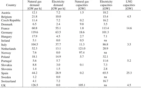
Table 4: Dataset
Country Natural gas demand [GW per h]
Electricity demand [GW per h]
Natural gas capacities
[GW]
Electricity capacities
[GW]
LNG capacities
[GW]
Austria 12.1 7.2 1.5 18.2
Belgium 21.8 10.0 15.4 4.5
Czech Republic 11.4 7.2 0.2 16.2
Denmark 6.5 2.4 9.8 3.5
France 60.8 55.1 1.8 113.4 14.6
Germany 119.6 63.5 18.6 101.3
Hungary 17.9 4.5 2.7 7.1
Ireland 5.1 0.0 0.5 na
Italy 104.5 37.7 11.3 86.8 3.5
Netherlands 52.3 13.1 121.0 20.9
Norway 7.6 0.0 97.4 na
Poland 18.1 14.9 5.7 32.1
Portugal 5.6 5.7 11.6 5.2
Slovakia 8.8 3.0 0.1 7.3
Slovenia 1.4 1.5 2.8
Spain 44.2 28.9 0.2 65.5 25.3
Sweden 1.2 0.0 na
Switzerland 4.1 7.2 16.7
UK 126.5 0.0 105.1 na 4.5
Figure 2: Base case, natural gas market, prices and congestion
!! !!
!!
!!
!! !! !! !! !!
!!
!!
>12 10 -12 9 - 10 8 - 9 7 - 8 6 - 7 <6
>12 10 -12 9 - 10 8 - 9 7 - 8 6 - 7 <6
Price €/MWh
[image:22.595.89.486.438.768.2]!! Congestion
Figure 3: Base case, electricity market, prices and congestion
>26 24 -26 22 - 24 20 - 22 18 - 20 16 - 18 <16
>26 24 -26 22 - 24 20 - 22 18 - 20 16 - 18 <16
Price €/MWh
!!
!!
!! !!
!!
Figure 4: Russian case, natural gas market, prices and congestion
!! !!
!! !! !! !! !! !! !!
!! !!
!!
>12 10 -12 9 - 10 8 - 9 7 - 8 6 - 7 <6
>12 10 -12 9 - 10 8 - 9 7 - 8 6 - 7 <6
Price €/MWh
[image:23.595.89.487.435.768.2]!! Congestion
Figure 5: Russian case, electricity market, prices and congestion
!!
!!
!! !!
!!
>26 24 -26 22 - 24 20 - 22 18 - 20 16 - 18 <16
>26 24 -26 22 - 24 20 - 22 18 - 20 16 - 18 <16
Price €/MWh
Figure 6: Emission case, natural gas market, prices and congestion
!! !!
!!
!! !!
!! !! !!
!!
!! !!
>12 10 -12 9 - 10 8 - 9 7 - 8 6 - 7 <6
>12 10 -12 9 - 10 8 - 9 7 - 8 6 - 7 <6
Price €/MWh
[image:24.595.90.486.436.767.2]!! Congestion
Figure 7: Emission case, electricity market, prices and congestion
!!
!! !!
!!
!! !!
>26 24 -26 22 - 24 20 - 22 18 - 20 16 - 18 <16
>26 24 -26 22 - 24 20 - 22 18 - 20 16 - 18 <16
Price €/MWh
![Table 2: Demand price outcomes [€/MWh]](https://thumb-us.123doks.com/thumbv2/123dok_us/7863602.737420/16.595.79.538.268.703/table-demand-price-outcomes-mwh.webp)