Stability, Chaos and Estimation of the Unknown Parameters of Habitat Destruction Model with Prey Predator Top Predator

ISSN Online: 2327-4379 ISSN Print: 2327-4352

Stability, Chaos and Estimation of the Unknown

Parameters of Habitat Destruction Model with

Prey-Predator-Top Predator

Saba Mohammed Alwan1*_{, Omalsad Hamood Odhah}2

1_{Department of Mathematics and Computer Science, College of Sciences, IBB University, Ibb, Yemen}

2_{Department of Mathematics, College of Sciences and Humanities, Prince Sattam Bin Abdulaziz University, Hotat Bany Tamim, Kingdom} of Saudi Arabia

Abstract

This paper is devoted to study the problem of stability, chaos behavior and parame-ters estimation of the habitat destruction model with three-species (prey, predator and top-predator). The mathematical formula of the model and its proposed interac-tions are presented. Some important special soluinterac-tions of systems are discussed. The stationary states of the model are derived. Local stability conditions for the stationary states are derived. Furthermore, the chaotic behavior of the model is discussed and presented graphically. Using Liapunov stability technique, the dynamic estimators of the unknown probabilities and their updating rules are derived. It is found that, the control laws are non-linear functions of the species densities. Numerical illustrative examples are carried out and presented graphically.

Keywords

Prey, Top-Predator, Three-Species, Estimation, Habitat Destruction, Lyapunov Function

1. Introduction

The habitat destruction is very important topic, which has received considerable atten-tion in the last years. It is sure that there is a direct correlaatten-tion between the preservaatten-tion of the environment, human civilization and progress, and vice versa. Some believe that the chaos is behind each destruction in the environment. In contrast, the others believe that the chaos provides a chance or space for the great changes and developments. It’s for sure that, the chaos is one of the main causes of the environmental destruction, but How to cite this paper: Alwan, S.M. and

Odhah, O.H. (2016) Stability, Chaos and Esti- mation of the Unknown Parameters of Habi-tat Destruction Model with Prey-Predator- Top Predator. Journal of Applied Mathe-matics and Physics, 4, 2254-2271.

http://dx.doi.org/10.4236/jamp.2016.412218

Received: November 19, 2016 Accepted: December 26, 2016 Published: December 29, 2016

Copyright © 2016 by authors and Scientific Research Publishing Inc. This work is licensed under the Creative Commons Attribution International License (CC BY 4.0).

it helps to achieve the needed balance in the environment. So, there is a controversy about whether the chaos has a positive role in the world or not. The balance of the en-vironment comes also, from the natural and bounded coexistence between the organ-isms.The future of the habitat should have a great interest. There are some studies that have focused on this, for example see [1].

When the habitat is no longer able to provide appropriate conditions for the life of its organisms, we can say that, the environment reached to the destruction stage, which is considered as an important factor causing extinction. It effects on various species not only directly but also indirectly. The accumulation of the destruction in a local area in-creases the risk of extinction in a bigger area and the increasing of the habitat destruc-tion caused an imbalance in the densities of the populadestruc-tions of prey and predator. So, we can say that, the causal relation between species extinction and the habitat destruc-tion is very complicated [2][3][4].

The variation of the total population size is determined by birth and the mortality rates [5]. In a closed population (i.e., no immigration) of size N, the change in popula-tion size for a change in time is given by ∆ ∆ = −N t

(

)

d are the birth, death and the growth rates per individual respectively. It is clearly that if l > 0, the population grows; if l < 0, the population heading towards extinction; if l = 0, no change in the population size. Recent models of competition indicate that, the effect of habitat destruction on coexisting between preys and predators is dependent on the ratio of extinction risk due to predation and prey colonization rate [6][7].

A lattice model represents the motion of a network of particles, where the motion is produced by forces acting between the neighboring particles. Lattice models also are used to simulate the structure of polymers and can exhibit its dynamic behaviors. Ma-thematically, the motion is governed by a system of ordinary differential equations. The behavior of the particles depends on the precise nature of the interaction. The main problems which have been treated involve the long time behavior of the system [8].

The results of this study are extend to the results that introduced by [2][3] where it found that the increase of habitat destruction leads to reduction in the chance of coex-istence of prey and predator, different patterns of extinction for the species (prey, pre-dator and top prepre-dator), and decrease in the oscillations in the densities of both species (prey and predator). Also, this study is considered as a complement for the results of the study [9] that concentrates on two-Species model, (prey-predator) which found that the system in general is unstable. In other hands, the chaotic behavior of the uncon-trolled system has seemed clear through the graphs of its limit cycles and some attrac-tors. The dynamic estimators of the unknown parameters and its updating rules over time are derived from the conditions of the asymptotic stability of the system around its steady states.

parame-ters and the updating [12]

The considered system contains three-species, which including prey, predator and top-predator. The assumed interactions and mathematical form of this model will be presented. Some special solutions of this system will be discussed. Chaos and linear sta-bility will be studied. The dynamic estimators of the unknown parameters of this model and its updating rules will be calculated.

This paper has the following structure. In Section 2, the lattice model and its as-sumed interactions are discussed and presented graphically. The mathematical formula model will be presented. Section 3 is devoted to study the chaos and linear stability analysis of the system. In Section 4, it is the analysis of some special solutions. Estima-tion of the unknown parameters and the updating rules are derived in SecEstima-tion 5. In Sec-tion 6, numerical soluSec-tions are derived and presented graphically. Finally, Conclusions are provided in Section 7.

2. The Lattice Model

In this section, the assumed interactions of the proposed model will be discussed and the mathematical formula will be presented.

Each site in the lattice can be labeled by X, Y, Z or O, where X, (or Y, Z) is the site occupied by prey (or predators), and O represents the vacant site. The assumed interac-tions of this model are given by [2]:

( )

( )

( )

( )

( )

( )

2 1.1 1.4

2 1.2 1.5

2 1.3 1.6

r r

r r

Y Z Z X O

X Y Y Y O

X O X Z O

 + → →  + → →   + → → _ (1)

The above interactions respectively represent two kinds of predation with probability 1, reproduction of prey with probability r0 and the deaths of the three-species prey, predator and top-predator, with probabilities r1, r2, r3 respectively. The transition ma-trix that presents the previous processes can be written as the following:

0

1

2

3

0

0 0 0 0

0 1 0 0 0 1 0 0 0

X Y Z

r r X r Y r Z                

Also, these interactions can be represented by Figure 1. In the lattice boundary, the barriers are putting as a link between neighboring sites probability p. which called bar-rier density. The interactions (1.1), (1.2) and (1.3) are assumed occur between neigh-boring lattice points as presented in Figure 1.

pc = 0.5 [1]. In contrast, when p takes an extremely small value, no barriers may con-nect with each other. Thus, p can be used as measures of the intensity of habitat de-struction.

The Mathematical Formula of the Model

The population dynamics of three-species model is described by the mean-field theory (MFT) [2], as the following form:

(

)

0 20 1 0 1 1 1 2 2 3 3

P = − r −p P P+r P+r P +r P (2.1)

(

)

1 20 1 0 1 1 1 2 1 2

P = r −p P P−r P− P P (2.2)

2 2 1 2 2 2 3 2 2

P = P P − P P−r P (2.3)

3 2 2 3 3 3

P = P P −r P (2.4)

where the dot represents the derivative with respect to time, P0, P1, P2 and P3 are the densities of O, X, Y and Z respectively, ri, i = 0, 1, 2, 3 are four unknown probabilities, which represent the probabilities of reproduction of prey, deaths of the prey, predator and top-predator, respectively. The probability p takes a non-critical value as explained previously.

The state variables of this system are subject to the following relationship

3

0

1

i i

P

=

=

∑

Therefore, for simplicity in our study, one can take just three equations instead of four, which are considered sufficient to demonstrate the chaotic behavior of the system and to estimate the unknown probabilities. Accordingly, using the relation in Equation (3), one can reduce the model in Equations (2) to the following model:

(

)(

)

1 20 1 1 1 2 3 1 1 1 2 1 2

P = r −p − −P P −P P−r P− P P (4.1)

2 2 1 2 2 2 3 2 2

P = P P − P P −r P (4.2)

3 2 2 3 3 3

P = P P−r P (4.3)

3. Chaos and Linear Stability Analysis

This section is devoted to study the local stability and the chaos behavior near the steady states of the three-spice model in Equations (4). The stationary states of the sys-tem in Equations (4) will be derived. The biological conditions for these steady states will be discussed. In addition, the instability conditions will be derived. Furthermore, some numerical solutions for the uncontrolled system and its instability, chaotic beha-vior and different attractors will be presented graphically.

3.1. The Stationary States

The stationary probabilities of the three-species model in Equations (4) can be ob-tained by setting the following simultaneous equations

0, 1, 2, 3

j

P = j= (5)

By solving this system analytically one can see the following stationary states. a) The first stationary probability of the system in Equations (4) is given by:

(

)

1 0, 0, 0

S = (6)

This solution corresponds to a vacuum-absorbing state. b) The second stationary probability of the system is given by:

3 2

2 0, ,

2 2

r r

S =_ − _

  (7)

Clearly, the density of the top-predator in this solution is negative. Due to that, this solution is biologically inadmissible.

c) The third stationary probability of the system is

1 3 , 0, 0

r

S α

α −

 

= _ _ (8)

where

(

)

0

2r 1 p 0

α = − ≥ ₍₉₎

The necessary condition for solution in Equation (8) to be biologically admissible is

1

r

α ≥ ₍₁₀₎

d) The fourth stationary probability of the system (4) is given by:

(

) (

)

2

4 , 1 2 2 2 , 0

2

r

S =_ α −r +α _

  (11)

The necessary condition for this solution to be biologically admissible is

(

)

1 2

2r 2 r

α ≥ −

e) The fifth stationary probability of the system (4) is given by:

2 3 1 3 3 2 3 1 3

5

1 1

, ,

2 4 2 2 2 4 2

r r r r r r r r r

S

α α

− + + +

 

=_ + − − − _

  (12)

The necessary condition for this solution to be biologically admissible is

(

) (

)

2 r r 2 r r

α ≥ + − − ₍₁₃₎

It is worth mentioning that, the condition in (13) is a sufficient condition to be S4 and S3 be biologically admissible because

(

) (

)

(

)

α ≥ + − − ≥ − ≥

3.2. Linear Stability Analysis

at its steady states and calculate the eigenvalues corresponding to each steady state. Then, we will determine whether these eigenvalues contain at least a positive root as a sufficient condition for instability [13] [14]. Also, we will seek to determine the insta-bility conditions for each steady state if needed.

The Jacobian matrix L of the system in Equation (4) evaluated at the steady state

, 1, 2, 3

j

P j= is given by:

(

)

(

)

(

)

1 2 3 1 2 1 1 1

2 1 3 2 2

3 2 3

1 2 2

2 2 2

0 2 2

P P P P P r P P

P P P r P

P P r

α α α α

 − − − − − − − + −      = − − −    −   

L (14)

Now let’s start by examining the instability of the steady states Si,1 1,= , 5 of

three-species model.

• _{The eigenvalues of the Jacobian matrix evaluated at S}1 are given by

11 r1, 12 r2 0, 13 r3 0

λ = −α λ = − < λ = − < ₍₁₅₎

Clearly, S1 is unstable if α >r1. The steady state S1 needs further stability analysis if 1

r

α < _{, because in this situation, we will get a critical case.}

• _{The eigenvalues of the Jacobian matrix evaluated at S}2 are given by solving the cha-racteristic equation, which is

(

)

(

)

(

)

(

)

2 3 3 1 2 2 2 3

1 r r 2 r r r r 0

α λ λ

 + − − + −  − =

  (16)

Therefore, the eigenvalues of L2 are the roots of Equation (16) which are given by

(

)

(

)

(

)

21 1 r2 r3 2 r3 r1 , , 22 r r2 3 23 r r2 3

λ =α + − − + λ = λ = − (17)

Due to the existence of a positive root in (17), the steady state S2 is absolutely unsta-ble.

• _{The eigenvalues of the Jacobian matrix evaluated at S}3 are given by

(

)

31 r1 , 232 r2 r1 , 033 r3

λ = −α λ = − + α− α λ = − < ₍₁₈₎

For this steady state, if α <r1, then λ >31 0, which is a sufficient condition for

insta-bility of S3. but, this condition makes the prey density in S3 has a negative value, there-fore this condition is biologically, not admissible. On other hand, if α >2r1

(

)

then λ >32 0. Therefore, this is a sufficient condition in order to be S3 unstable.

• _{The eigenvalues of the Jacobian matrix evaluated at S}4 are given by the roots of the following characteristic equation:

(

)

(

)

2 3 4 4 1 4 1 2

2A − −r λ _λ +α λA +2A A α+2 _=0 (19)

where

(

)

1 2 2

1 2 2 ,

2

r

A r A α

α −

= =

+ (20) For the linear factor, the necessary condition for its root to be positive value is

(

) (

)

α> + − − + < (21)

It is worth mentioning, for the quadratic polynomial in Equation (19), the second coefficient αA1>0 is positive because of A1=r2 2>0 and α =2r0

(

)

the third coefficient is positive under the condition in (21). Since all the real coefficients of the quadratic polynomial in Equation (19) are positive, using the Routh’s stability criterion [15], then all the roots of quadratic polynomial are negative if the condition (21) is satisfied. Accordingly, S4 is unstable under the condition in (21) and the stability decision needs further stability analysis

• _{The eigenvalues of the Jacobian matrix evaluated at S}5 are given by the roots of the following characteristic equation.

(

)

2

5 5 B1 5 r3 2B3 B1 2B1 0

λ λ_ −α λ + +α + _= (22)

where

2 3 1 3 2 3 1 3

1 3

1 1

,

2 4 2 2 4 2

r r r r r r r r

B B

α α

− + + +

= + − = − − (23)

Without solving the polynomial between the rectangular brackets in (22) and using Descartes rule of signs to determine the number of positive zeros of the polynomial, one can find that, the first coefficient is positive, and by simple calculation, it is easy to see that if

(

) (

)

2 r r 2 r r , r r 2

α < + + − + < ₍₂₄₎

then, B1<0; and B3<0. Under this condition, the second coefficient of the

poly-nomial between the rectangular brackets in Equation (23) will be positive and the third will be negative. In this case the polynomial has one variation in sign. Therefore, the polynomial has one positive real zeros and the other is negative. So, we can conclude that, S5 is unstable if the condition in (24) is satisfied.

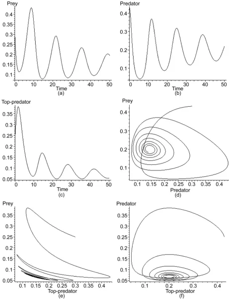
In the following we will present graphically, the system behavior over time, which il-lustrate the oscillatory behavior of the system.

In this figure, all state variables of the uncontrolled system in Equations (4) that ap-pear in (a, b, c) have an oscillatory behavior. For limit cycles that apap-pear in (d, e, f), all the neighboring trajectories tend to a limit-cycle at time tends to infinity, causing the so-called a stable limit-cycle, which indicates that the system has an oscillatory beha-vior.

In the following we will present a special behavior of this system which is a periodic orbits which called attractors as in Figure 3. Attractors is a special behavior, which generated by the dynamical system and steadily developing as long as there is no barrier

All graphs of uncontrolled densities, limit cycles and attractors in Figure 2 and Fig-ure 3 well agree with the previous linear stability analysis that indicates that the habitat destruction model with three-species has a high chaotic behavior.

4. Analysis of Some Special Solutions

Figure 3. Different attractors of the habitat destruction model of the three-species for the following rates, parameters and initial densities:

0

r r1 r2 r3 p P1 0 P2 0 P3 0

0.012 0.0001 0.007 0.009 0.12 0.17 0.01 0.2

0.01 0.008 0.07 0.07 0.08 0.25 0.01 0.6

0.012 0.0001 0.007 0.009 0.57 0.25 0.006 0.15

0.01 0.001 0.49 0.005 0.5 0.25 0.003 0.15

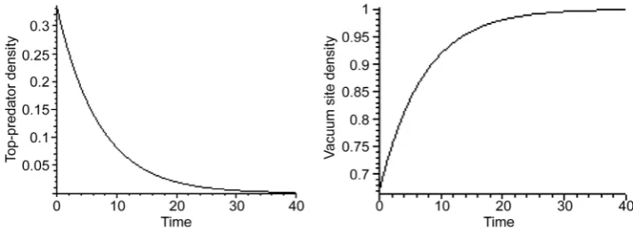
• _{The first special solution occurs when both prey and predator are absent, that is P}1 = 0 and P2 = 0. In this case, the top-predator decreases exponentially with rate r3 as indicants in the following growth equation:

3 3

3 30e 0 1 30e

r t r t

P =P − P = −P − (25)

Figure 4. Simultaneous evanescence and growth of top-predator and empty sites respectively in the absence case of prey and predator at P3 0=0.33; 3r =0.14.

• The second special solution occurs in the absence of both prey and predator, that is P1 = 0 and P3 = 0. This situation is similar to the previous case, therefore, the preda-tor will be decreased exponentially with rate r2, and the empty sites density increases over time to tend to one. This situation represents also, a vacuum-absorbing state. • Another special solution occurs when both of the predator and top-predator are ab-sent, that is P2 = 0 and P3 = 0. In this case the model in Equation (4) will be reduced to the contact percolation process [2], that is a one-species model we have where the birth and death processes of species X are assumed, which can be presented as

2

X+ →O X and X →O. In this case the system will take the following reducing

form

(

)

0 20 1 1 0 1 1

P = − r −p P P +r P (26.1)

(

)

1 20 1 1 0 1 1

P = r −p P P −r P (26.2)

By solving this system, we will take the following prey population growth:

(

)

( )

( )

( )

( )

1 1

1 1

1 1₀ 1 1₀

1 0

1₀ 1₀

e 1 e

1 e 1 e

r r

t t

r r

t t

r P r P

P P

P P

α α

α α

α

α α

− −

− −

− +

= =

+ + (27)

where

(

)

0

2r 1 p 0

α = − ≥ ₍₂₈₎

Equation (27) indicates that, the density of the prey tends to

(

)

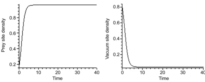
to infinity. If the death probability of the prey be zero, then the prey population has a logistic growth and all sites of the lattice will be occupied by prey as t tends to infinity

[16][17] to make a prey-absorbing state as shown in Figure 5.

It is useful to notice that, in order the result in (27) be biologically admissible, the following condition must be satisfied:

(

)

1 0 1 at 0.5 0 2 1

r r r p r

α≥ ⇔ ≥ = ∀ ≤ ≤ (29)

Figure 5. Simultaneous growth of both of prey and empty densities in the absence case of preda-tor at P1 0=0.23, 1r =0.05, α=1.2.

(

)

0 20 1 1 0 2 2

P = − r − p P P +r P (30.1)

(

)

1 2 1 2 20 1 1 0 1 1

P = − P P + r −p P P −r P (30.2)

2 2 1 2 2 2

P = P P −r P (30.3)

which has been studied in [9]. It is found that, one absorbing stationary state and two active stationary states. It is found also that, these stationary states are unstable. Fur-thermore, this system showed a chaotic behavior.

• _{In the absence of prey, P}1 = 0, we will obtain another two-species model (predator- top predator) as given below

2 2 2 3 2 2

P = − P P −r P (31.1)

3 2 2 3 3 3

P = P P −r P (31.2)

This subsystem has two steady states, which are

( )

11 0, 0 12 ,

2 2

r r

e = e =_ − _

  (32)

The Jacobian matrix Jsub1 of the subsystem (31) evaluated at the steady sate

, 2, 3

k

P k= is given by:

3 2 2

3 2 3

2 2

2 2

P r P

P P r

− − − 

=  ₋ 

 

Jsub1 (33)

The Jacobian matrices Jsub11 and Jsub12 at e11 and e12 respectively, are given below

2 3

3 2

0 0

,

0 0

r r

r r

− −

   

=_{ } =_{ }

− _− _

 

Jsub11 Jsub12 (34)

The eigenvalues of Jsub11 are

1 0, 3 0

r r

− < − < ₍₃₅₎

The eigenvalues of Jsub12 are

2 3 0, 2 3 0

Clearly, the steady state e11 is stable, while the steady state e12 is absolutely unstable. Therefore, the subsystem (31) is unstable at least in one dimension.

• _{The following considered special solution occurs when the predator is absent, that is} P2 = 0 In this case, the three-species system will be reduced to a subsystem of two- species model with prey-top predator as will present below

(

)

1 1 1 1 3 1

P =P_α − −P P −r_ (37.1)

3 3 3

P = −r P (37.2)

This system has the following two stationary solutions:

( )

21 0, 0 22 1 , 0

r

e e

α

 

= = −_{ }

  (38)

The Jacobian matrix Jsub2 of the subsystem in Equation (37) evaluated at its steady states P k_k, =1, 3 is given by:

(

)

3

1 2 0

P P r P

r α α  − − − −  =   −    

Jsub2 (39)

Therefore, the Jacobian matrices at e21 and e22 respectively, are given by:

1 1 1

3 3

0

0 0

r r r

r r

α− −α −α

   

=_{ } =_{ }

− −

   

Jsub21 Jsub22 (40)

and the eigenvalues of Jsub21 are:

1 3 0

r r

α − − < ₍₄₁₎

and the eigenvalues of Jsub22 are:

1 3 0

r−α − <r (42)

Clearly, the steady state e21

( )

(

)

(

)

1 1

r r

α< α> _{and the stability decision needs more stability analysis if} α =r₁, in which one get a critical case. One can conclude that the subsystem (37) is unstable at least in one direction.

• _{The last special solution occurs when no vacant sites in the lattice, that is P}0 = 0. In this case the processes: reproduction of prey, death of prey and death of predator will be disabled, and only the predation process will be remained. As a result of this, the density of predator has the following form

(

)

(

)

(

)

2 2₀

2 2 1 2

t

2₀ 2₀

2 e ₁

1 2 e 1 2 e

t t P P P P P = =

+ + (43)

Figure 6. Simultaneous growth of the predator site density and the prey site density in the ab-sence of empty sites at the initial value P_{2 0}=0.82.

5. Estimations of the Unknown Probabilities

This section is devoted to derive the estimators of the unknown probabilities of the three-species model of habitat destruction (4). The dynamic estimators of the unknown probability ri, i = 0, 1, 2, 3 and its updating rules will be calculated from the conditions of the asymptotic stability of the system (4) near its stationary solutions Sk, k = 1, 2, ∙∙∙, 5 with assistance of some feedback variables e1, e2 and e3.

At the beginning, we will develop the mathematical formula of the habitat destruc-tion model of three-species with unknown probabilities in (4) to become as follows:

(

)(

)

1 2ˆ0 1 1 1 2 3 1 ˆ1 1 2 1 2 1

P = r −p − −P P −P P−r P− P P +e (44.1)

2 2 1 2 2 2 3 ˆ2 2 2

P = P P − P P −r P +e (44.2)

3 2 2 3 ˆ3 3 3

P = P P −r P +e (44.3)

where rˆi are the estimators of the unknown probabilities ri, i = 0, 1, 2, 3 of the system (4). The model in Equations (44) has unstable stationary solution if e1=e2 =e3 =0.

This solution is given by

( )

(

)

ˆi i 0,1, 2, 3 , s s, 1, 2, 3

r t =r i= P =P s= (45)

The problem now is equivalent to stabilizing of these steady states and determining the updating rules rˆ1 of the estimators rˆi of the system unknown probabilities ri with help of the controllers es,

(

)

The Lyapunov function of the system (4) that will be used can be considered as the following positive definite form

(

)

(

)

(

)

2

1 0

1 1

ˆ ˆ

, ;

2 2

j s i i s s

i s

V P r t P P r r

= =

=

∑

∑

and its time derivative is given by

(

)

(

)(

)

(

)

[

]

(

)

[

]

(

)

1 1 0 1 2 3 1 1 1 1 2 1

2 2 1 2 2 3 2 2 2 3 3 2 3 3 3 3

3

0

ˆ ˆ

2 1 1 2

ˆ ˆ

2 2 2

ˆ ˆ

_{s s s}

s

V P P r p P P P P r P P P e

P P P P P P r P e P P P P r P e

r r r

=

 

= − _ − − − − − − + _

+ − − − + − − +

+

∑



By choosing the controllers as follows:

(

)

(

)(

)

1 1 1 1 2 1 2 1 1 20 1 1 1 2 3 1,

e = −k P−P + P P +r P− r −p − −P P −P P (48.1)

(

)

2 2 2 2 2 2 3 2 2 2 1 2,

e = −k P −P + P P +r P − P P (48.2)

(

)

3 3 3 3 3 3 2 2 3.

e = −k P −P +r P − P P (48.3)

and by substituting (48) in (47), one can get that the appropriate choice for the updat-ing rules rˆ_i for V to be a negative definite function are given by

( )

(

) (

)

(

)

(

)

0 0 0 0 1 1 1 2 3 1

ˆ ˆ 2 1 1 ,

r t = −m r −r − −p P −P − −P P −P P (49.1)

( )

(

)

(

)

1 1 1 1 1 1 1

ˆ ˆ ,

r t = −m r −r +P P−P (49.2)

( )

(

)

(

)

2 2 2 2 2 2 2

ˆ ˆ ,

r t = −m r −r +P P −P (49.3)

( )

(

)

(

)

3 3 3 3 3 3 3

ˆ ˆ .

r t = −m r −r +P P −P (49.4)

where ks and mi are non-negative control constants.

By substituting the choices (48) and (49) in (47), V will be a negative definite func-tion, which proves the asymptotic stability of the solution (45) in Lyapunov sense. Fur-ther that, this solution is globally asymptotically stable since V is radially unbounded

[18][19]. And by substituting Equation (48) in the controlled system in Equation (44), in addition Equation (9) we get the following closed system of nonlinear deferential equations following form:

(

)

(

)(

)(

)

(

)

1 1 1 1 2 ˆ0 0 1 1 1 2 3 1 ˆ1 1 1

P = −k P−P + r −r −p − −P P −P P− r−r P (50.1)

(

)

(

)

2 2 2 2 2 ˆ2 2 ,

P = −k P −P −P r −r (50.2)

(

)

(

)

3 3 3 3 3 ˆ3 3 ,

P = −k P −P −P r −r (50.3)

( )

(

) (

)(

)

(

)

0 0 0 0 1 2 3 1 1 1

ˆ ˆ 2 1 1 ,

r t = −m r −r − −p − −P P −P P P−P (50.4)

( )

(

)

(

)

1 1 1 1 1 1 1

ˆ ˆ ,

r t = −m r −r +P P−P (50.5)

( )

(

)

(

)

2 2 2 2 2 2 2

ˆ ˆ ,

r t = −m r −r +P P −P (50.6)

( )

(

)

(

)

3 3 3 3 3 3 3

ˆ ˆ .

r t = −m r −r +P P −P (50.7)

This system can be used to study the dynamics of the habitat destruction model of three-species with unknown probabilities. Since this system is nonlinear, its solution will be numerical as will be seen bellow.

6. Numerical Solution

r0 r1 r2 r3 p m0 m1 m2 m3 k1 K2 K3

0.7 0.2 0.45 0.3 0.35 3 1 5 2 1.5 1 2

0 0 ˆ

r rˆ1 0 rˆ2 0 rˆ3 0 P1 0 P2 0 P3 0

0.3 0.6 0.45 0.2 0.1 0.6 0.25

Figure 7 indicates that the controlled densities of the three species converge to the steady state over time. The steady states are presented by the dotted lines.

For the same values of probabilities, parameters and initial densities above, let us represent the estimators of the unknown probabilities.

In Figure 8, it is shown that, the estimators r iˆ, =0,1, 2, converge to the assumed

real values ri over time, where the assumed real values are represented by the dotted

Figure 7. The controlled densities of (a) prey, (b) predator, and (c) top-predator sites of the ha-bitat destruction model of three-species for the following values of probabilities, parameters and initial densities.

lines. It is necessary to know that the very small differences between the assumed real values and the estimated values are be due to the necessary approximations in the nu-merical method of solution.

7. Conclusions

This paper is devoted to study the linear stability, chaos and estimation of the unknown parameters of the habitat destruction model with prey-predator and top-predator. Us-ing the linear stability analysis, it is found that, this system has a high chaotic behavior. The dynamic estimators of the unknown parameters and its updating rules over time are derived from the conditions of the asymptotic stability of the system around its steady states. The controller laws are found as non-linear functions of the species densi-ties. Numerical examples for the controlled system are carried out and presented graphically.

The chaotic behavior of this system gives us a reason to study the optimal control for this system in future.

References

[1] Ergazaki, M. and Ampatzidis, G. (2012) Students’ Reasoning about the Future of Disturbed or Protected Ecosystems & the Idea of the “Balance of Nature”. Research in Science Educa-tion, 42, 511-530.https://doi.org/10.1007/s11165-011-9208-7

[2] Nakagiri, N. and Tainaka, K. (2004)Indirect Effects of Habitat Destruction in Model Co-systems. Ecological Modelling, 174, 103-114.

https://doi.org/10.1016/j.ecolmodel.2003.12.047

[3] Szwabinski, J. and Pekalski, A. (2006) Effects of Random Habitat Destruction in a Preda-tor-Prey Model. Physica A, 360, 59-70. https://doi.org/10.1016/j.physa.2005.05.079

[4] Nakagiri, N., Tainaka, K. and Tao, T. (2001) Indirect Relation between Extinction and Ha-bitat Destruction. Ecological Modelling, 137, 109-118.

https://doi.org/10.1016/S0304-3800(00)00417-8

[5] El-Gohary, A. (2005) Optimal Control of Stochastic Lattice of Prey-Predator Models. Ap-plied Mathematics and Computation, 160, 15-28.

https://doi.org/10.1016/S0096-3003(03)00668-4

[6] Klausmeier, C.A. (1998) Extinction in Multispecies and Spatially Explicit Models of Habitat Destruction. The American Naturalist, 152. https://doi.org/10.1086/286170

[7] Swihart, R., Feng, Z., Slade, N., Mason, D. and Gehring, T. (2001) Effects of Habitat De-struction and Resource Supplementation in a Predator-Prey Metapopulation Model. Jour-nal of Theoretical Biology, 210, 287-303. https://doi.org/10.1006/jtbi.2001.2304

[8] Liggtt, T.M. (1985) Interacting Particle Systems. Springer-Verlag, Inc., New York.

[9] Alwan, S. and El-Gohary, A. (2011) Chaos, Estimation and Optimal Control of Habitat De-struction Model with Uncertain Parameters. Computers and Mathematics with Applica-tions, 62, 4089-4099.

[10] Al-Mahdi, A. and Khirallah, M. (2016) Bifurcation Analysis of a Model of Cancer. Euro-pean Scientific Journal, 12, 68-83.

[12] Alwan, S. (2016) Chaos Behavior and Estimation of the Unknown Parameters of Stochastic Lattice Gas for Prey-Predator Model Pair-Approximation. Applied Mathematics, 7, 1765- 1779. https://doi.org/10.4236/am.2016.715148

[13] Hacker, T. (1970) Flight Stability and Control. American Elsevier Publishing Company, Inc., New York.

[14] Cook, P.M. (1994) Nonlinear Dynamical Systems. Prentice Hall International, Upper Sad-dle River.

[15] Ogata, K. (1997) Modern Control Engineering. Prentice-Hall, Inc., Upper Saddle River. [16] El-Gohary, A. and Bukhari, F. (2003) Optimal Control of Stochastic Prey-Predator Models.

Applied Mathematics and Computation, 146, 403-415.

https://doi.org/10.1016/S0096-3003(02)00592-1

[17] El-Gohary, A. and Al-Ruzaiza, A. (2007) Chaos and Adaptive Control in Two Prey, One Predator System with Nonlinear Feedback. Chaos, Solitons and Fractals, 34, 443-453.

https://doi.org/10.1016/j.chaos.2006.03.101

[18] Brogan, W.L. (1982.) Modern Control Theory. Prentice-Hall, Inc., Upper Saddle River. [19] El-Gohary, A. (2002) Global Stabilization of a Rotational Motion of a Rigid Body Using

Rotors System.Applied Mathematics and Computation, 133, 297-307.

https://doi.org/10.1016/S0096-3003(01)00235-1

Submit or recommend next manuscript to SCIRP and we will provide best service for you:

Accepting pre-submission inquiries through Email, Facebook, LinkedIn, Twitter, etc. A wide selection of journals (inclusive of 9 subjects, more than 200 journals)

Providing 24-hour high-quality service User-friendly online submission system Fair and swift peer-review system

Efficient typesetting and proofreading procedure

Display of the result of downloads and visits, as well as the number of cited articles Maximum dissemination of your research work