The influence of variable selection methods on the accuracy of bankruptcy prediction models

Munich Personal RePEc Archive

The influence of variable selection

methods on the accuracy of bankruptcy

prediction models

du Jardin, Philippe

Edhec Business School

January 2012

Online at

https://mpra.ub.uni-muenchen.de/44383/

du Jardin, P., 2012, The influence of variable selection methods on the accuracy of bankruptcy prediction models, Bankers, Markets & Investors, issue 116, January, pp. 20–39.

1

The influence of variable selection methods on the

accuracy of bankruptcy prediction models

Philippe du Jardin Professor

Edhec Business School 393, Promenade des Anglais

BP 3116 06202 Nice Cedex 3

Email: [email protected]

Abstract – Over the last four decades, bankruptcy prediction has given rise to an extensive body of literature, the aim of which was to assess the conditions under which forecasting models perform effectively. Of all the parameters that may influence model accuracy, one has rarely been discussed: the influence of the variable selection method. The aim of our research is to evaluate the prediction accuracy of models designed with various classification techniques and variables selection methods. As a result, we demonstrate that a search strategy cannot be designed without considering the characteristics of the modeling technique and that the fit between the variable selection method and the technique used to design models is a key factor in performance.

Key words – bankruptcy, prediction model, variable selection JEL classification – G33, C52

Introduction

Since the late 1960’s, many researchers have been working on how to design bankruptcy prediction models with statistical techniques. These researchers addressed two main issues. The first focused on modeling techniques and tried to assess their experimental performance conditions.1 The aim was to provide an understanding of the ability of classification or regression techniques to solve bankruptcy prediction problems and create accurate models. Appendix 1 presents the modeling techniques used in the main research studies which aimed to analyze and compare their respective predictive power. This area of research was based on the seminal work of Beaver (1966), who demonstrated the ability of financial ratios to serve as reliable proxies for measuring a risk of financial failure, and of Altman (1968), who first assessed the usefulness of multivariate statistical techniques to design forecasting rules. Since then, more than fifty different methods have been used in this field.

The second main issue focused on explanatory variables that might be used to design models. The aim was to find the best predictors in terms of model accuracy as well as to determine the factors that might influence these predictors. For instance, Back et al. (1994), analyzed the extent to which a financial-variable-based model (a model using balance sheet or income statement figures) might perform better than a financial-ratio-based model (a model using ratios that are constructed by dividing two financial variables). Mossman et al. (1998) did a similar experiment and compared results obtained with ratio-based models and models based on financial market variables. Lussier (1995) considered the problem of

2 building a bankruptcy model with qualitative variables that described both the leaders and the business of firms. Atiya (2001) compared a ratio-based model with a ratio- and financial- market-variable-based model to analyze their respective accuracy. Mensah (1984) analyzed the influence of the timeframe where the variables are measured on the accuracy of a model. Platt and Platt (1990) focused on the influence of the sector on the bankruptcy probability, while Pompe and Bilderbeek (2005) examined the influence of macro-economic factors.

Nevertheless, research on modeling techniques or variable selection was not really intended to analyze the fit of the former and the latter. Indeed, when the authors sought an effective means of improving the accuracy of a prediction rule, one of the following strategies was used to choose explanatory variables: variables were selected because they were considered “good” predictors in the financial literature, for their performance on univariate statistical tests (t test, F test, correlation test), or as a result of automatic search procedures using evaluation criteria tailored to discriminant analysis (Wilks lambda) or logistic regression (likelihood ratio). Only very few studies used other criteria. Appendix 2 illustrates the methods or criteria used during the variable selection process for research presented in appendix 1.

If we analyze these tables, we may wonder to what extent a selection procedure that takes into account only individual characteristics of variables or that fails to take into account the inductive algorithm (John et al., 1994; Kohavi, 1995) may affect the results of a classification rule. We may also wonder, as suggested by Leray and Gallinari (1998), if it is relevant to use selection techniques based on parametric tests in conjunction with non-parametric modeling methods.

Up to now, no research has tried to address the variable selection issue and the contribution of variable selection methods to the accuracy of financial failure models.

Thus, the aim of our research is to assess the influence of variable selection processes on the accuracy of a model and study the fit of modeling methods and variable selection techniques for designing bankruptcy models.

This paper is organized as follows. In section 1, we describe the methods traditionally used to identify variables when the aim of the research is to build the most reliable bankruptcy prediction models. In section 2, we describe the methods and sample used in our experiments. Then, in section 3, we present and discuss our empirical results, and, in conclusion, we summarize the main findings of the study.

1 Literature review

3 modeling technique. Indeed, a “good” variable or set of variables does not exist in itself; a “good” set of variables seems to be in part the result of the characteristics of the set itself and, in part, that of the fit between this set and the modeling method (John et al., 1994; Kohavi, 1995). As a consequence, choosing bankruptcy predictors solely for their popularity in the literature leads to the belief that only their intrinsic properties may play a significant role.

The second main selection method relies on statistics. Variables are chosen based on statistical tests. These tests are often univariate and deal either with the individual discrimination ability of a variable or with correlations with other variables. However, assessing a variable’s individual discrimination power is far from sufficient to estimate its effective contribution to the performance of a model. Moreover, these tests often rely on linear assumptions and are thus reliable only in linear contexts. As there is some evidence that the relationship between bankruptcy probability and a set of financial variables behave in a non-linear manner (Laitinen and Laitinen, 2000), these tests may have misleading results.

The third method of selecting variables is more sophisticated than the former because it uses an automated selection process. But this process is very often the same: it relies on a stepwise search and an evaluation criterion based either on a distance measure that evaluates the contri-bution of a variable to the discrimination between groups (Wilks Lambda) or on a likelihood criterion (Likelihood ratio). These two criteria are optimized for discriminant analysis and logistic regression respectively. But are these criteria still efficient when used in conjunction with other techniques? There is absolutely no reason to believe that a variance criterion such as a Wilks Lambda may perform well with a neural network, for example. On the contrary, it might be of no use or harmful with such a method (Leray and Gallinari, 1998).2

The three above-mentioned methods of selecting variables are those commonly used in the bankruptcy literature. Only a few studies implement other strategies. Some rely on a conceptual model to choose their final predictors (Aziz et al., 1988; Laitinen and Laitinen, 2000). Others rely on a financial expert (Dimitras et al., 1999). We may also find some authors who use statistical means other than univariate methods: factor analysis, multiple regression, classification trees, genetic algorithms, sensitivity analyses, and so on. Two of these techniques are very often used. First is the genetic algorithm (Back et al., 1994; Wallrafen et al., 1996; Sexton et al., 2003; Brabazon and Keenan, 2004). A genetic algorithm has the advantage of estimating a solution based on the method used to design the model (induction algorithm) and not solely on the intrinsic characteristics of the variables. So, because it does not impose any constraint on the evaluation criterion, it can be considered a valuable alternative when the modeling technique is non-parametric. The selection will then be done based on the performance that the induction algorithm achieves when using the variables that are being evaluated. Second are sensitivity techniques (Tyree and Long, 1996; Charalambous et al., 2000; Bose and Pal, 2006), which are widely used with artificial neural networks. The selection is then done using heuristics that attempt to reduce the complexity of network architecture: input nodes and connections are pruned during the search process, leading to the elimination of inappropriate and irrelevant variables in accordance with the evaluation criterion.

As a consequence, the sets of variables selected to design prediction models are often under-optimized regarding the modeling technique because the criterion used to assess their legitimacy does not always make sense. Is it really relevant to use a Wilks Lambda with a neural network to design a bankruptcy model? What about a likelihood evaluation criterion

4 used in conjunction with a method that is different from logistic regression? Is it better to use a sensitivity measure with an artificial neural network than a likelihood criterion? Is it pertinent to use the induction algorithm during the selection process (wrapper approach), despite the fact that it is time consuming, or is it better to evaluate the variables independently from this algorithm (filter approach)? These are a few questions that have not received, for the moment, the attention that they deserve.

It is therefore worth noting that many authors strongly recommend comparing the results obtained with different classification or regression techniques even though they do not apply the same reasoning to the selection methods that determine the variables for these techniques. Appendix 2 is quite significant in this regard. For this reason, the aim of our research is to use “modeling method-variable selection technique” pair analysis to examine the influence of the latter on the former in terms of prediction accuracy and answer the questions posed above. We focus mainly on the evaluation criteria used with selection methods, without taking into account other criteria, such as the correlation of variables, that can also be used to select variables, but that are not a part of a selection method in itself.To the best of our knowledge, only one study (Back et al., 1996) has compared a pair of sets of variables optimized for a discriminant analysis, a logistic regression and a neural network, but only to analyze the differences between the models in terms of accuracy over different prediction timeframes (one, two or three years).

2 Samples and methods

2.1 Samples and variables

We first selected companies in the retail sector because in France this sector traditionally accounts for the largest percentage of failed firms.

Within this set of companies, we selected firms with an asset structure as homogenous as possible to control for the size effect (Gupta, 1969) and to allow comparisons of ratios. As there is no rule for drawing a homogenous sample, we ran an Anova and a Mann-Whitney test on several breakdowns to find the most homogenous group. These tests were computed on both failed and non-failed companies. Finally, the breakdown of companies into one group with assets of more than €750,000 and another with assets of less than €750,000 was the breakdown in which the differences between the two groups, measured with all ratios, were the largest. It was also the breakdown that allowed a relatively large sample size.

We then selected accounting data and computed only financial ratios. Data were collected within a single year, 2002, and we included just one variable (shareholder funds) from the previous year (2001). When we selected healthy companies, we chose only companies in very good shape, as suggested by Malecot (1991), that is, companies that were still in business in 2005. Moreover, we selected companies in operation for at least four years, because during the very first years of their lives, young, healthy companies have a financial structure similar to that of failed companies. Bankrupt companies were selected only if they were liquidated or reorganized in 2003, and at least 16 months after the publication of the annual report from 2002, so as to avoid any intentional distortion of financial statements. We tried to design a well-balanced sample of young and old firms, because young companies are usually much more likely to go bankrupt than older ones. Finally, we selected bankrupt companies for which accounting data were available in 2002, and shareholder funds available in 2001, and for which bankruptcy was declared (liquidation or reorganization) by court decision in 2003.

5 We then selected a second sample (test sample), made up of companies from the same sector and with the same amounts of assets, but data were from 2003, with one variable from 2002 (shareholder funds). All bankrupt companies in the database that were liquidated or reorganized by court decision in 2004 were selected. Healthy companies were randomly selected from among those that were active in 2004. This second sample was made up of 880 healthy and 880 bankrupt firms. Companies in this second sample were not already included in the first sample. This sample was used to estimate model accuracy. None of these companies used consolidated data.

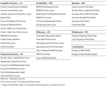
We then chose a set of 41 initial variables that can be broken down into seven categories that best describe company financial profiles: liquidity-solvency, financial structure, profitability, efficiency, turnover, withdrawal and contribution (table 1).

Table 1: Initial set of variables

Liquidity-Solvency – LI Profitability – PR Rotation – RO

Current Assets/Current Liabilities EBITDA/Permanent Assets Current Assets/Total Sales Current Assets/Total Assets EBITDA/Total Assets Net Op. Work. Capital/Total Sales (Current Assets-Inventory)/Tot. Assets Profit before Tax/Shareholder Funds Accounts Receivable/Total Sales Quick Ratio EBIT/Total Assets Accounts Payable/Total Sales Current Liabilities/Total Assets Net Income/Shareholder Funds Inventory/Total Sales Financial Debt/Cash Flow Net Income/Total Assets Cash/Total Sales (Cash + Mark. Sec.)/Total Sales

(Cash + Mark. Sec.)/Total Assets Efficiency – EF Withdrawal – WI

EBITDA/Total Sales Total Sales/Shareholder Funds Financial Expenses/Total Sales Cash/Current Liabilities Total Sales/Total Assets Labor Expenses/Total Sales Cash/Total Assets Operating Cash Flow/Total Assets

Cash/Total Debt Operating Cash Flow/Total Sales Contribution

Gross Trading Profit/Total Sales Change in Other Debts

Financial Structure – FS EBIT/Total Sales Change in Shareholders Equity*

Net Op. Work. Capital/Total Assets Value Added/Total Sales Shareholder Funds/Total Assets

Long Term Debt/Shareholder Funds Long Term Debt/Total Assets Total Debt/Shareholder Funds Total Debt/Total Assets

Mark. Sec. : Marketable Securities

Net Op. Work. Capital : Net Operating Working Capital

* Change in Shareholders Equity was calculated without taking into account profit and loss

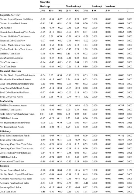
6 Table 2: Characteristics of the variables belonging to the learning and validation samples Quartiles – Normality test and tests for differences between the two groups

Quartiles

Bankrupt Non-bankrupt Bankrupt Non-bank.

25% 50% 75% 25% 50% 75% S-W S-W t U

Liquidity-Solvency

Current Assets/Current Liabilities -0.86 -0.54 -0.27 -0.16 0.20 0.77 0.000 0.000 0.000 0.000 Current Assets/Total Assets -0.41 0.46 0.91 -0.68 0.04 0.70 0.000 0.000 0.008 0.000 Quick Ratio -0.85 -0.55 -0.22 -0.31 0.25 0.95 0.000 0.000 0.000 0.000 Current Assets-Inventory)/Tot. Assets -0.95 -0.11 0.63 -0.69 0.21 0.81 0.000 0.000 0.063 0.039 Current Liabilities/Total Assets -0.15 0.29 0.70 -0.79 -0.53 -0.28 0.000 0.024 0.000 0.000 Financial Debt/Cash Flow -0.07 -0.05 -0.03 -0.04 -0.04 -0.02 0.000 0.000 0.669 0.000 (Cash + Mark. Sec.)/Total Sales -0.78 -0.68 -0.38 -0.39 0.13 1.13 0.000 0.000 0.000 0.000 (Cash + Mark. Sec.)/Total Assets -0.85 -0.73 -0.35 -0.43 0.28 1.28 0.000 0.000 0.000 0.000 EBITDA/Total Sales -0.96 -0.30 0.02 0.15 0.35 0.72 0.000 0.000 0.000 0.000 Cash/Current Liabilities -0.70 -0.47 -0.36 -0.21 0.23 0.95 0.000 0.000 0.000 0.000 Cash/Total Assets -0.94 -0.42 -0.13 -0.10 0.44 1.19 0.000 0.095 0.000 0.000 Cash/Total Debt -0.68 -0.44 -0.33 -0.21 0.18 0.89 0.000 0.000 0.000 0.000

Financial Structure

Net Op. Work. Capital/Total Assets -0.54 0.05 0.50 -0.10 0.21 0.53 0.000 0.473 0.000 0.000 Shareholder Funds/Total Assets -0.69 -0.15 0.07 0.34 0.49 0.73 0.000 0.000 0.000 0.000 Long Term Debt/Shareholder Funds -0.10 -0.04 0.02 -0.03 -0.01 0.02 0.000 0.000 0.681 0.000 Long Term Debt/Total Assets -0.57 -0.14 0.50 -0.63 -0.33 0.10 0.000 0.000 0.000 0.000 Total Debt/Shareholder Funds -0.77 -0.49 -0.33 -0.05 0.18 0.73 0.000 0.000 0.000 0.000 Total Debt/Total Assets -0.08 0.15 0.72 -0.74 -0.48 -0.32 0.000 0.000 0.000 0.000

Profitability

EBITDA/Permanent Assets -0.11 -0.06 -0.02 -0.04 -0.03 -0.01 0.000 0.000 0.743 0.000 EBITDA/Total Assets -0.81 -0.30 0.03 0.20 0.39 0.68 0.000 0.000 0.000 0.000 Profit before Tax/Shareholder Funds 0.01 0.06 0.08 0.08 0.09 0.11 0.000 0.000 0.003 0.000 EBIT/Total Assets -0.87 -0.23 0.11 0.27 0.43 0.70 0.000 0.000 0.000 0.000 Net Income/Shareholder Funds -0.09 0.00 0.10 -0.01 0.01 0.04 0.000 0.000 0.651 0.026 Net Income/Total Assets -0.86 -0.24 0.11 0.29 0.41 0.70 0.000 0.000 0.000 0.000

Efficiency

Total Sales/Shareholder Funds -0.11 -0.05 0.14 0.01 0.04 0.09 0.000 0.000 0.142 0.000 Total Sales/Total Assets -0.59 -0.29 0.31 -0.61 -0.29 0.24 0.000 0.000 0.878 0.994 Operating Cash Flow/Total Sales -0.64 -0.28 0.18 -0.19 0.12 0.55 0.000 0.000 0.000 0.000 Operating Cash Flow/Total Assets -0.67 -0.28 0.26 -0.18 0.16 0.50 0.000 0.000 0.000 0.000 Gross Trading Profit/Total Sales -0.64 -0.10 0.47 -0.55 0.08 0.71 0.000 0.005 0.001 0.006 EBIT/Total Sales -0.95 -0.24 0.09 0.21 0.40 0.69 0.000 0.000 0.000 0.000 Value Added/Total Sales -0.89 -0.46 0.24 -0.32 0.24 0.99 0.000 0.001 0.000 0.000

Rotation

7

Withdrawal

Financial Expenses/Total Sales -0.26 -0.19 -0.03 -0.30 -0.27 -0.22 0.000 0.000 0.046 0.000 Labor Expenses/Total Sales -0.73 -0.17 0.47 -0.67 -0.11 0.51 0.000 0.000 0.431 0.995

Contribution

Change in Other Debts -0.09 -0.05 0.18 -0.09 -0.05 -0.01 0.000 0.000 0.139 0.026 Change in Shareholders Equity 0.25 0.25 0.25 -0.44 0.15 0.25 0.000 0.000 0.000 0.000 S-W: p-value of a Shapiro-Wilks normality test

t: p-value of a Student t test for differences between the means of the two groups U: p-value of a Mann-Whitney test for the equality of the sum of ranks of each group

2.2 Modeling and variable selection methods

2.2.1 Modeling methods

We chose modeling methods for their popularity in the financial literature. Of the more than 50 regression or discriminant techniques, three predominate: discriminant analysis, logistic regression and a special type of neural network, known as multilayer perceptron, trained with a steepest descent method. We then selected these three methods.

2.2.1.1 Discriminant analysis

The aim of discriminant analysis is to classify objects in two or several groups on the basis of a set of variables. To design the classification rule, the algorithm attempts to derive the linear combination of independent variables that will best discriminate between groups defined beforehand, which in our case are healthy and failed companies. This is achieved using a statistical method of maximizing the between-group variance relative to the within-group variance. Discriminant analysis then computes a score z according to:

n nx w x

w x

w   

 ...

z _{1 1 2 2}

where wi are the discriminant weights and xi are the independent variables (e.g., financial ratios). Thus, each company receives a single composite discriminant score which is then compared to a cut-off value which determines the group the company belongs to.

Discriminant analysis is a robust, parametric statistical technique that relies on a number of assumptions being met: the explanatory variables within each group must follow a multivariate normal distribution, the variance-covariance matrices of the groups must be equal and the correlation of the explanatory variables must be as low as possible. However, these assumptions are sometimes difficult to meet. Moreover, the assumption of linearity between function output and the input variables does not always apply and the groups being considered are often non-linearly separable.

2.2.1.2 Logistic regression

Logistic regression is often used to overcome some of the constraints that discriminant analysis imposes on data, and it tolerates a certain degree of non-linearity between the input and the output of a model. Indeed, with logistic regression there are no mandatory assumptions, rather a supposition that the explanatory variables fit a logistic curve. A logistic regression function computes a probability score z for each observation to be classified, where:

  



 n i xiwi

e 1

8 It computes the coefficients w_i of the function using maximum likelihood estimation. As with a discriminant function, an observation will be classified in one of two groups depending on its score.

2.2.1.3 Neural network

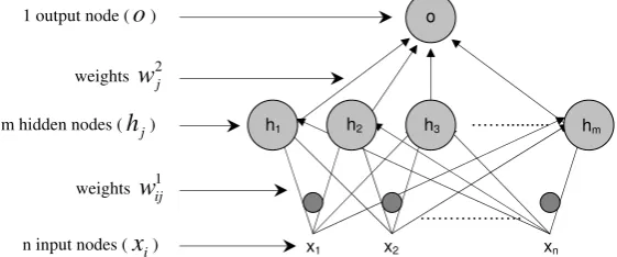
An artificial neural network, like discriminant analysis or logistic regression, is a commonly used classification method. But, unlike discriminant analysis and logistic regression, neural networks do not represent the relationship between the explanatory variables and the dependant variable with an equation. This relationship is expressed as a matrix containing values, also called weights, that represent the strength of connections between nodes or neurons. In this study, a multilayer perceptron (MLP) with a single hidden layer was used to perform the classification task.

Figure 1: Architecture of a multilayer perceptron with n input nodes, m hidden nodes and one output node

Figure 1 depicts an example of multilayer perceptron architecture. From a general point of view, this network is made of an input layer (vector x), one or several hidden layers (vector

h in this example) and an output layer made of one or several nodes (o in this example).

The layers are linked together as shown in Figure 1, and the relationships between nodes are represented by weights. In that example above, the weights 1

ij

w represent the relationships

between the nodes of the input layer and the nodes of the hidden layer, and the weights 2

j

w

represent the relationships between the nodes of the hidden layer and the output node.

If one considers a classification task of n observations into two groups to be achieved by the neural network described above, the vector x represents the explanatory variables, and o

represents the result of the classification: class 1 or class 2. The values go through the network as a result of the activation function of each node. The activation function transforms input into output. The input value of a hidden node hj is the weighted sum of the input nodes



n i 1xiwij

1 _{and its output is ( )} 1

1



n i xiwij

f . The output of the output node o is f(



The weights of the network are computed through a learning process. The network thus learns how to correctly classify a set of observations for which output is known. During the learning phase, the network processes a set of inputs and compares its resulting outputs against the desired outputs. The error (the difference between the network's calculated values for the output node and the correct values) is then calculated, and weights are adjusted proportionally to this error until a stopping criterion is reached. During this process, network

x1 x2

……….….….

xn

1 output node (o)

……...

m hidden nodes (h_j)

n input nodes (x_i)

o

h1 h2 h3 hm

weights w1_ij

9 weights are tuned to values that allow the network to achieve a low classification error with data used during the learning phase, and that also allow good prediction ability when using data that were not used during this phase. Once the learning process is done, the network can be used for forecasting tasks.

Unlike discriminant analysis, this kind of network does not require distributional assumptions of the explanatory variables and is able to model all types of non-linear functions between the input and the output of a model. This universal approximation capability, assessed by Hornik et al. (1990), Hornik (1991) and Hornik et al. (1994), and the ability to build parsimonious models make them powerful models. Indeed, not only are these networks able to model relationships that discriminant analysis cannot but they can also design models that are more parsimonious than those built with other non-linear techniques, such as polynomials. They can therefore build models with the same accuracy as traditional non-linear techniques, but with fewer adjustable parameters, or models with much better accuracy with the same number of parameters.

As far as the network is concerned, we could not use it without defining its parameters, which ultimately depend on the variables to be used. However, the network was intended to be used during the selection process, to find the relevant variables. A question is thus raised: must we determine the parameters during selection or before? The fist solution, in which one seeks an optimal combination of parameters and variables simultaneously, is time consuming. The second solution, in which the parameters are defined a priori, does not necessarily lead to the best architecture, but it is faster than the first one. In the literature, network parameters are sometimes determined a priori and sometimes, as in Back et al. (1997), who used a constant number of neurons, arbitrarily. Others may introduce a certain degree of variability, while testing different sizes of the hidden layer, but with a fairly limited number of nodes; among those who do so are Back et al. (1994), Back, Laitinen and Sere (1996), Sexton et al. (2003) and Brabazon and Keenan (2004), all of whom selected variables while testing different hidden layer architectures. From a general standpoint, when a network is used during a selection process, its parameters are determined a priori. We chose to determine network parameters a priori so as to assess only the influence of selection criteria on model accuracy, not that of network architecture.

To compute these parameters, we ran a set of experiments. We drew at random 50 sets of variables from among those first selected. For each set of variables, we tested several combinations of parameters: learning steps (from 0.1 to 0.5, with a 0.1 step), momentum terms (from 0.5 to 0.9, with a 0.1 step), weight decays, with one decay per layer (from 10-5 to 10-2 with a 10-1 step), and the number of hidden nodes (from 2 to 10). We used only one hidden layer. All these figures were derived from those traditionally used with an MLP by the authors we reviewed, although there is no guarantee that they are optimum or close to an optimum. They were also defined in keeping with the number of combinations to explore. Tests to define the length of the learning process were likewise run. We stopped the learning process after 1,000 iterations, because the error was stable on average.

Then, for each combination, we estimated the error with a 10-cross validation procedure and data from 2002. The error was averaged over the 50 sets, and we finally selected the parameters that led to the best solution: four hidden nodes, 0.4 for the learning step, 0.4 for the momentum term, 10-4 and 10-3 for the decay parameters between the input layer and the hidden layer, and between the hidden layer and the output node.

2.2.2 Variable selection methods

10 Wilks Lambda to compare variable subsets and determine the “best” one. This technique was complemented with two others: a forward stepwise search and a backward stepwise search, with a likelihood statistic as an evaluation criterion of the solutions and a Chi2 as a stopping criterion. We then selected four of the most commonly used methods especially designed for neural networks (Leray and Gallinari, 1998), three of them evaluated the variables without using the inductive algorithm (filter methods) and one used the algorithm as an evaluation function (wrapper method). The first is a zero-order technique which uses the evaluation criteria designed by Yacoub and Bennani (1997). The second is a first-order method that uses the first derivatives of network parameters with respect to variables as an evaluation criterion. The third is a second-order technique inspired by weight pruning methods. For the latter, a weight is pruned if its saliency, as the relevance criterion is known, is low. Leray and Gallinari (1998) proposed to extend these methods for variable selection. Their method, early cell damage, computes the saliency of a variable as a function of its weight saliencies. A variable is pruned if it has the lowest saliency. The last one relies on the evaluation of an out-of-sample error calculated with the neural network (error criterion). To estimate this error, each sample used during the selection, the process for which is presented below, was divided into two parts: 250 firms (125 healthy and 125 bankrupt) were used during the learning phase, and the other 250 firms were used to compute the error.

We therefore chose one method that fits discriminant analysis (Wilks Lambda criterion), two that fit logistic regression (likelihood criterion), and four that fit neural networks (error, zero first and second-order criteria).

With all these criteria, we used only a backward search rather than a forward or a stepwise search. As the search procedure involved successive removal of variables, the network was retrained after each removal, and the selection procedure was performed until all variables were removed. In the end, the set of variables that led to the lowest error was chosen.

Finally, to select variables, 1,000 random bootstrap samples were drawn from the dataset for the year 2002 (500 firms). Each bootstrap sample involved selection. To identify important variables, those that were included in more than 70% of the selection results were included in the final models. To avoid discarding potentially relevant but highly correlated variables, variable pairs in which one or both variables were included in more than 90% of the bootstrap selections were considered pairs containing a relevant variable. Then, for each identified pair, the variable that occurred in most of the selection results was ultimately chosen. Once these selections were made, the entire process was repeated to choose the final subsets.

This procedure was used with the seven selection strategies.

2.3 Model development

We used the following procedure to develop the models. The year 2002 sample was randomly divided into two sub-samples: a learning sample A of 450 companies and a validation sample T of 50 companies. Twenty-five bootstrap samples were drawn from A and, for each selected set of variables, used to estimate as many models as bootstrap samples. Finally, the resulting models were used to classify the observations of sample T. These steps were repeated 100 times.

We used such a procedure to reduce the variance of the error of prediction arising from data instability. Indeed, financial ratios are always far from being normally distributed and contain many outliers. As a consequence, a small change in the learning data may produce a substantial change in the results. To reduce the influence of these outliers, we have chosen this bootstrap scheme (Breiman, 1996; Grandvalet, 2004).

11 We used this procedure with all pairs of “modeling method-selection criterion” for which the evaluation criterion suited the classification technique. We then computed seven sets of 25 x 100 models: discriminant analysis-Wilks Lambda, likelihood criterion-logistic regression and forward search, likelihood criterion-logistic regression and backward search, neural network-error criterion, neural network-zero order criterion, neural network-first order criterion and neural network-second order criterion. For each set, the 25 x 100 models were used to estimate the out-of-sample error rate, along with the test sample (1,480 companies, data for the year 2003).

We then estimated several other sets of models for which the evaluation criterion did not fit the classification technique. We used discriminant analysis with the two sets of variables selected with a likelihood criterion and the sets chosen with the four criteria optimized for the neural network; we then used logistic regression with the variables selected with a Wilks Lambda and the sets optimized for the network, and finally we used the neural network with the set optimized for discriminant analysis and the sets optimized for logistic regression.

For each “modeling method-selection criterion” pair, we estimated 25 x 100 models with data from 2002 (validation sample) and we estimated the generalization error of these models with data from 2003 (test sample).

To compute the generalization error of each “modeling method-selection criterion” pair, we first calculated the predicted class of each company achieved by each of the 2,500 models as follows:            _{^ *} * ^ * model using calculated company of score if (failed) 0 model using calculated company of score if (healthy) 1 y j i y y j i y y ij ij ij

where *

ij

y is the predicted class of company i using model j, y_ij^ the score of company i calcu-lated using model j and y*the cut-off value used to determine the boundary between the two classes. The cut-off value was assessed so as to maximize the global rate of correct classifications.

We then calculated the final predicted class of each company, averaging the predictions of the 2,500 models as follows:

                     







where M 2,500 is the number of models andy_i*the final predicted class of company i. We then estimated the classification error of each company as follows:

         i i i i i i y y y y y e if 0 ed undetermin is or if 1 * * *

were ei is the classification error of company i,

*

i

y the predicted class of company i and i

y the current class of company i.

Finally, we assessed the global classification error, type I (misclassifying a failed firm) and type II (misclassifying a healthy firm) errors of each “modeling method-selection criterion” pair as follows:

12 where e_iis the classification error of company i and N the sample size (1,480 companies).





 NF

j F j N

e

1

error I

Type





 NH

k H k N

e

1

error II Type

where e_jis the classification error of failed company j, N_Fthe number of failed firms (740

companies), ek the classification error of healthy company k and NHthe number of healthy firms (740 companies).

All our experiments and results were achieved between 2006 and 2009.

3 Results

3.1 Selected variables and structure of the models

Tables 3, 4 and 5 show the seven sets of variables that appeared in the selection results. Those that were chosen in more than 70% of the results were included in the final models. Each variable name is followed by its frequency of selection and its category (LI: Liquidity-solvency; FS: Financial structure; PR: Profitability; EF: Efficiency; RO: Rotation; WI: Withdrawal; CO: Contribution). Variables that appeared in a least three models are highlighted in gray.

Appendix 3 shows the results of a factor analysis applied to each set of variables so as to present the correlation of the predictors.

Table 3: Selected variables using a Wilks Lambda criterion

Variables included into the model

Frequency of selection

Category

Cash/Total Assets 93.4% LI Total Debt/Shareholder Funds 91.1% FS Cash/Total Debt 88.7% LI (Cash + Mark. Sec.)/Total Assets 87.5% LI EBIT/Total Assets 81.2% PR EBITDA/Total Assets 76.8% PR Shareholder Funds/Total Assets 72.2% FS

Table 4: Selected variables using a likelihood criterion

Search: Backward Stepwise

Variables included into the model

Frequency of selection

Category

13

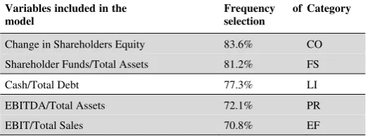
Search: Forward Stepwise

Variables included in the model

Frequency of selection

Category

Change in Shareholders Equity 83.6% CO Shareholder Funds/Total Assets 81.2% FS Cash/Total Debt 77.3% LI EBITDA/Total Assets 72.1% PR EBIT/Total Sales 70.8% EF

Table 5: Selected variables using neural network criteria

Error

Variables included in the model

Frequency of selection

Category

Shareholder Funds/Tot. Assets 91.8% FS EBIT/Total Assets 86.2% PR Cash/Current Liabilities 83.1% LI Change in Shareholders Equity 81.8% CO EBITDA/Total Assets 76.6% PR EBIT/Total Sales 76.1% EF (Cash + Mark. Sec.)/Tot. Assets 74.9% LI Accounts Receivable/Tot. Sales 70.6% RO

0 Order

Search: Forward Stepwise Variables included in the model

Frequency of selection

Category

Net Income/Total Assets 86.7% PR (Cash + Mark. Sec.)/Tot. Assets 84.3% LI Shareholder Funds/Tot. Assets 83.8% FS EBITDA/Total Assets 80.9% PR Cash/Current Liabilities 78.2% LI Total Debt/Total Assets 74.5% FS Change in Shareholders Equity 73.9% CO Cash/Total Sales 71.5% RO

1st _Order

Variables included in the model

Frequency of selection

Category

14

2d _Order

Variables included in the model

Frequency of selection

Category

EBITDA/Total Assets 81.60% PR EBIT/Total Sales 79.10% EF Current Assets/Current Liabilities 78.60% LI Cash/Total Debt 76.90% LI Total Debt/Total Assets 72.80% FS Cash/Total Sales 71.40% RO

When we analyze each set of variables presented in tables 3, 4 and 5, we can notice that the variance-based criterion (Wilks Lambda) results in a weaker representation of financial failure than that of the two other sets of criteria (likelihood and criteria optimized for the neural network) because only three financial dimensions are taken into account: liquidity-solvency, profitability and financial structure. These dimensions can be considered basic dimensions since the legal definition of financial failure relies mostly on liquidity and profitability, regardless of the country.

With the two other sets of criteria, the situation is somewhat different. The second, which relies on a likelihood statistic, resulted in the use of variables that are related to liquidity-solvency, profitability and financial structure but has complemented these dimensions with three others: contribution, efficiency and rotation. The third and last set, which relies on criteria well suited for the neural network, shows the same characteristics as the second, but not in the same order of importance. Indeed, if we count the variables of each model according to the dimension they belong to, and take into account their rank, we see that the second set of criteria leads to models which rely, in decreasing order of importance, on financial structure, contribution, profitability and liquidity-solvency. The third set of criteria, if it considers profitability as the main dimension, complemented the list with financial structure, liquidity-solvency, and then contribution, efficiency and rotation.

These differences in pecking order probably depend on the number of selection criteria used with each modeling technique. But other factors may also have influenced the results. It seems that the last two sets of criteria have “captured” relationships that the first one was unable to find within the data. It is worth noting that the variable Change in Shareholders Equity, which plays a significant role for many companies in our samples, has been completely ignored by the first criterion. Therefore, the fact that this variable was included in a few models depends less on its intrinsic importance than on the relationships it was involved in. We can observe how various selection methods, depending on the way they take into account linearities and non-linearities, may represent or reveal differences in model structures. We can also observe how a likelihood criterion and neural-based criteria may lead to a similar vision of failure from a conceptual point of view, and how a variance criterion leads to a different representation. Perhaps the performance of the models designed with these sets of variables will confirm their “proximity”, but this time in terms of prediction accuracy.

15 the structure of the basic model. Finally, all these models demonstrate that there are basic failure indicators that are not completely contingent and that do not depend solely on a variable selection procedure.

3.2 Variable discrimination power

After analyzing the similarities and differences of the seven models, we studied the discrimination power of all the variables from different points of view to assess to what extent univariate statistical tests (i.e., tests for differences between two means) may be considered reliable means of achieving a selection or pre-selection of variables, as stated in the literature, and particularly of selecting predictors to be used with non-linear techniques.

3.2.1 Most frequently selected variables

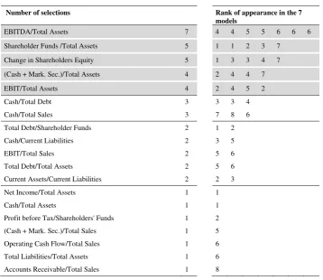
Table 6 ranks the variables by frequency of appearance in the seven sets of variables. Only one ratio appeared in all models (EBITDA/Total Assets) but four other ratios are shared by at least four models (Shareholder Funds /Total Assets, Change in Shareholders Equity, (Cash + Marketable Securities)/Total Assets and EBIT/Total Assets).

Table 6: Ranking of the variables

Number of selections Rank of appearance in the 7 models

EBITDA/Total Assets 7 4 4 5 5 6 6 6 Shareholder Funds /Total Assets 5 1 1 2 3 7

Change in Shareholders Equity 5 1 3 3 4 7 (Cash + Mark. Sec.)/Total Assets 4 2 4 4 7 EBIT/Total Assets 4 2 4 5 2

Cash/Total Debt 3 3 3 4 Cash/Total Sales 3 7 8 6 Total Debt/Shareholder Funds 2 1 2 Cash/Current Liabilities 2 3 5 EBIT/Total Sales 2 5 6 Total Debt/Total Assets 2 5 6 Current Assets/Current Liabilities 2 2 3 Net Income/Total Assets 1 1 Cash/Total Assets 1 1 Profit before Tax/Shareholders' Funds 1 2

(Cash + Mark. Sec.)/Total Sales 1 5 Operating Cash Flow/Total Sales 1 6

Total Liabilities/Total Assets 1 6 Accounts Receivable/Total Sales 1 8

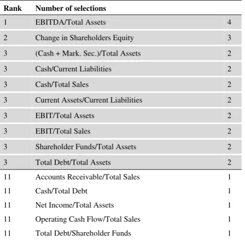
3.2.2 Most frequently selected variables when using a neural network

16 Table 7: Ranking of the variables selected with a neural network

Rank Number of selections

1 EBITDA/Total Assets 4 2 Change in Shareholders Equity 3 3 (Cash + Mark. Sec.)/Total Assets 2 3 Cash/Current Liabilities 2 3 Cash/Total Sales 2 3 Current Assets/Current Liabilities 2 3 EBIT/Total Assets 2 3 EBIT/Total Sales 2 3 Shareholder Funds/Total Assets 2 3 Total Debt/Total Assets 2 11 Accounts Receivable/Total Sales 1 11 Cash/Total Debt 1 11 Net Income/Total Assets 1 11 Operating Cash Flow/Total Sales 1 11 Total Debt/Shareholder Funds 1

3.2.3 Relationship between different measures of discrimination

Table 8 ranks the variables by their discrimination ability, as assessed by an F test. In this table, we have added their rank as it appears in table 7. The first half of table 8 (line 1 to line 21) shows the variables for which the F test reveals the highest discrimination power. This part of the table also contains fourteen of the fifteen variables selected with the neural network. This result indicates that there is a relationship between a parametric measure of discrimination and all the others we used in this study and which are non-parametric. However, this relationship is fairly rough because the two rankings are quite different. For instance, as table 8 shows, the five variables that are most frequently selected with a neural network (EBITDA/Total Assets, Shareholder Funds/Total Assets, Change in Shareholders Equity, (Cash + Marketable Securities)/Total Assets and EBIT/Total Assets) are ranked 4th, 6th, 20th, 12th and 3rd respectively. By contrast, variables with high discrimination ability, such as EBITDA/Total Sales, Cash/Total Assets or Current Liabilities/Total Assets are not selected with any selection techniques.

As a consequence, using a t or an F test for selection or pre-selection of the input to a neural network is unreliable as these tests may lead to the choice of unnecessary variables as well as to the removal of variables of great interest. Such might well have been the case here, with the Change in Shareholders Equity, for which the F test is quite low even though this variable is in fact relevant according to the neural network. Indeed, selection with a Wilks Lambda removes this variable. But when the value of an F test falls below a certain level, the only other variable selected is Accounts Receivable/Total Sales (which is selected only once). Table 8: Rank of the variables by F test

F p-val. Rank1

17

5 Net Income/Total Assets 210.01 0.000 11 6 Shareholder Funds/Total Assets 207.59 0.000 3 7 Total Debt/Total Assets 202.20 0.000 3 8 Total Debt/Shareholder Funds 201.14 0.000 11 9 Cash/Total Assets 195.01 0.000 10 Cash/Total Sales 179.60 0.000 3 11 Current Liabilities/Total Assets 179.32 0.000 12 (Cash + Mark. Sec.)/Total Assets 171.62 0.000 3 13 Cash/Current Liabilities 168.19 0.000 3 14 Cash/Total Debt 150.50 0.000 11 15 (Cash + Mark. Sec.)/Total Sales 145.63 0.000 16 Current Assets/Current Liabilities 133.77 0.000 3 17 Quick Ratio 131.30 0.000 18 Accounts Payable/Total Sales 85.95 0.000 19 Value Added/Total Sales 68.37 0.000 20 Change in Shareholders Equity 44.29 0.000 2 21 Operating Cash Flow/Total Sales 28.57 0.000 11 22 Net Operating Working Capital/Total Assets 27.21 0.000 23 Net Operating Working Capital/Total Sales 21.10 0.000 24 Operating Cash Flow/Total Assets 19.40 0.000 25 Long Term Debt/Total Assets 19.32 0.000 26 Inventory/Total Sales 16.00 0.000 27 Accounts Receivable/Total Sales 13.38 0.000 11 28 Gross Trading Profit/Total Sales 10.53 0.001 29 Profit before Tax/Shareholder Funds 8.97 0.003 30 Current Assets/Total Assets 7.13 0.008 31 Current Assets/Total Sales 4.83 0.028 32 Financial Expenses/Total Sales 4.04 0.045 33 (Current Assets-Inventory)/Total Assets 3.47 0.063 34 Change in Other Debts 2.20 0.139 35 Total Sales/Shareholder’ Funds 2.16 0.142 36 Labor Expenses/Total Sales 0.62 0.431 37 Net Income/Shareholder Funds 0.20 0.651 38 Financial Debt/Cash 0.18 0.669 39 Long Term Debt/Shareholder Funds 0.17 0.681 40 EBITDA/Permanent Assets 0.11 0.743

41 Total Sales/Total Assets 0.02 0.878

1 _{Rank of the variables in Table 7}

3.3 Model accuracy

We then analyzed the relationship between modeling techniques and variable selection methods. The aim was to investigate whether there were any pairs that perform better than others and to study the behavior of a neural network while using sets of variables that were optimized for other methods.

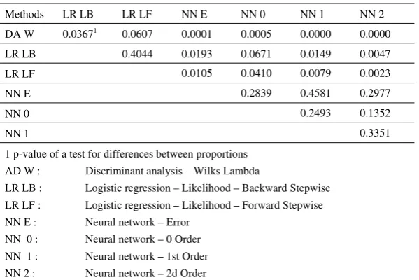
18 and neural network–error, zero-order, first-order and second-order criteria. As table 9 shows, the neural network outperforms discriminant analysis and to a lesser extent logistic regression. Indeed, the best result – 88.92% – is achieved with a neural network on the test samples, followed by that for logistic regression with 86.02% and discriminant analysis with 83.86%. Table 10 shows the results of a test for differences in correct classification rates. These tests indicate that the results achieved with a neural network are significantly different from those achieved with discriminant analysis. However, at the conventional significance level of 5%, neither the difference between logistic regression (using a forward search) and discriminant analysis nor the difference between logistic regression (using a backward search) and the neural network (using a zero-order criterion) is significant.

Table 9: Model accuracy for “modeling-technique–variable–selection-method” pairs calculated on test samples

DA Wilks

Step.

LR Lik. B Step.

LR Lik. F Step.

NN Error B

NN 0 Order B

NN 1st _Order

B

NN 2d _Order

B Non-bankrupt 86.93% 86.48% 88.86% 87.27% 85.45% 88.86% 88.30%

Bankrupt 80.80% 85.57% 82.61% 89.43% 90.00% 88.07% 89.55% Total 83.86% 86.02% 85.74% 88.35% 87.73% 88.47% 88.92%

DA: Discriminant analysis – LR: Logistic regression – NN: Neural network Lik.: Likelihood – B: Backward – F: Forward – Step.: Stepwise

Table 10: Tests for differences between correct classification rates

Methods LR LB LR LF NN E NN 0 NN 1 NN 2 DA W 0.03671 _{0.0607 0.0001 0.0005 0.0000 0.0000}

LR LB 0.4044 0.0193 0.0671 0.0149 0.0047 LR LF 0.0105 0.0410 0.0079 0.0023 NN E 0.2839 0.4581 0.2977 NN 0 0.2493 0.1352 NN 1 0.3351 1 p-value of a test for differences between proportions

AD W : Discriminant analysis – Wilks Lambda

LR LB : Logistic regression – Likelihood – Backward Stepwise LR LF : Logistic regression – Likelihood – Forward Stepwise NN E : Neural network – Error

NN 0 : Neural network – 0 Order NN 1 : Neural network – 1st Order NN 2 : Neural network – 2d Order

We then analyzed the results obtained when a modeling technique is used with a selection procedure for which the fit is not deemed acceptable. Table 11 displays the results obtained with the set of variables selected with a Wilks Lambda and those selected with a likelihood criterion. Table 12 gives the results calculated with the four sets of variables optimized for a neural network.

19 which discriminant analysis is founded. It is little wonder then that variables that cannot satisfactorily classify a high percentage of firms with discriminant analysis are unable to provide satisfactory results with other methods; the models built with logistic regression and the neural network produce similar results from a statistical point of view. Therefore, this criterion is ill-suited to a neural network.

Table 11: Model accuracy according to modeling techniques and two variable selection criteria (Wilks Lambda–Likelihood) calculated on test samples

Wilks Lambda Stepwise

Likelihood Backward Stepwise

Likelihood Forward Stepwise DA LR RN DA LR RN DA LR RN Non-bankrupt 86.93% 80.23% 80.80% 83.52% 86.48% 83.52% 80.91% 88.86% 84.20% Bankrupt 80.80% 81.36% 77.27% 79.77% 85.57% 84.32% 81.70% 82.61% 82.61% Total 83.86% 80.80% 79.03% 81.65% 86.02% 83.92% 81.31% 85.74% 83.41%

Test for differences between correct classification rates

Test for differences between correct classification rates

Test for differences between correct classification rates

Methods LR NN LR NN LR NN DA 0.00851 _{0.0001 DA 0.0002 0.0371 DA 0.0002 0.0509}

LR 0.0961 LR 0.0405 LR 0.0279

1 p-value of a test for differences between proportions

DA : Discriminant analysis – LR : Logistic regression – NN : Neural network

The sets of variables that are selected with a likelihood criterion result in less accurate results with discriminant analysis than with logistic regression – 81.65% – as opposed to 86.02% with a backward search, and 81.31% as opposed to 85.74% with a forward search. However, with a neural network, the results of these two sets are slightly higher – 83.92% and 83.41% – than the results obtained with discriminant analysis.

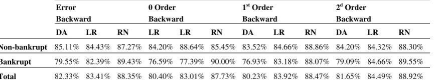
The second-order criterion achieved an accuracy of 88.92% compared to 84.49% for logistic regression, and 81.65% for discriminant analysis. The discrepancy between the results of the three methods is broadly similar with an error criterion, with respective figures for correct classification of 88.35%, 83.41% and 82.33%. But with a zero-order criterion, as well as a first-order criterion, there is a slight increase. With a zero-order the figures are 87.73%, 83.01% and 80.40%, with a first-order they are 88.47%, 83.92 % and 80.23%. In all cases, the differences between the neural network and the other two methods are statistically significant. Table 12: Model accuracy by modeling technique and four variable selection criteria (Error, Zero, First and Second-Order) calculated on test samples

Error Backward

0 Order Backward

1st _Order

Backward

2d _Order

Backward

20

Test for differences between correct classification rates

Test for differences between correct classification rates

Test for differences between correct classification rates

Test for differences between correct classification rates Methods LR NN LR NN LR NN LR NN

DA 0.19771 _0.0000

DA 0.0225 0.0000 DA 0.0021 0.0000 DA 0.0123 0.0000

LR 0.0000 LR 0.0000 LR 0.0000 LR 0.0001 1 p-value of a test for differences between proportions

DA : Discriminant analysis – LR : Logistic regression – NN : Neural network

Therefore, the neural network leads to better results than logistic regression and discriminant analysis, especially with a second-order criterion, even though the differences between this criterion and the three others are not great.

When developed with appropriate variables, neural models are thus slightly more reliable than logistic or discriminant models. Moreover, logistic models outperformed discriminant models and the differences are statistically significant in three of four instances.

All performance measures presented in this study confirm, in a way, the conclusions we draw from the structure of the models. On one hand, the representation of financial failure suggested by the set of variables selected with a Wilks Lambda is, in terms of its underlying financial dimensions, less complex and less multiform than that suggested by the other two sets. This fact may explain the different forecasting results; this set is inefficient when used with a discriminant analysis and does not work particularly well with other methods. On the other hand, the previously described similarities that we found between the sets of variables selected with a likelihood criterion and those selected with criteria suited to the neural network seemed to be reflected in forecasted results because they are somewhat close: the best models in each criterion category achieved results on test data that differ by less than two points, and most of these sets of variables produce accurate results, both with logistic regression and with the neural network. However, the differences most likely reflect the very characteristics of the methods rather than the content of variables themselves. The neural network is less accurate than logistic regression when variables that do not fit its properties are used. At the same time, the neural network is able to achieve better results when the variables are selected with criteria that meet its characteristics.

The accuracy of a model is in part the result of the intrinsic properties of the modeling technique and in part that of the fit between this technique and the variable selection procedure involved in its design. In the field of bankruptcy prediction, all the experiments that have been carried out with large samples show that both financial ratios and a probability of bankruptcy behave in a non-linear manner. It is precisely for this reason that, as long as this non-linearity cannot be taken into account, it is difficult to develop accurate models. Although using a selection criterion that fits logistic regression to design a neural model may be relevant, the choice of a criterion that fits discriminant analysis for the same purpose should not be recommended. It is necessary, at the very least, to consider other solutions.

Conclusion

21 Second, differences and similarities in the sets of variables can also be found in the way these sets reflect the financial dimensions of bankruptcy. The first set, selected with a Wilks Lambda, embodies a representation of failure conceptually poorer than those embodied by the two others, while the other two sets make it possible to draw a standard profile of this phenomenon for the firms represented in our samples. They point to the operating cycle of the companies and the operating working capital as key issues of financial failure. A firm that is able to run its activity is profitable and liquid. This profitability is essential in the event of financial threats because, for this kind of company, there are very few external sources of financing. With the first set of variables, the influence of the operating cycle is not great, and the role of the shareholders as a key factor of recovery in the event of financial difficulties was completely ignored.

22 Appendix 1

Main research which aimed to compare or assess the predictive power of regression or classification techniques

Authors Methods Main objective

Agarwal (1999) NN-DA-AN To assess the efficiency of a new method (abductive network) to build a financial failure prediction model and to compare its predictive accuracy against the accuracy of a neural network Alam et al. (2000) NN-FC To compare the ability of a fuzzy clustering method to

correctly classify failed banks against the ability of a Kohonen map dealing with the same issue

Alfaro et al. (2008) AB-NN-DA-CT To compare the respective predictive ability of a neural network and AdaBoost

Altman (1968) DA To demonstrate that ratio analysis may be a relevant analytical technique in assessing the performance of the business enterprise

Altman et al. (1994) NN-DA-LR To compare the predictive ability of three different methods: discriminant analysis, logistic regression and a neural network Baranoff et al. (2000) SR-LR-PR-CLR-CPR To compare the predictive ability of different methods Barniv and Hershbarger (1990) DA-LR-NPDA To find the relevant variables which may be used to assess the

degree of solvency of insurance companies and to assess the efficiency of different multivariate methods to monitor this solvency

Barniv and Raveh (1989) DA-LR-PR-NPDA To test the ability of a new non-parametric method to predict corporate failure

Boritz and Kennedy (1995) NN-DA-LR-PR-NPDA-QDA To examine the effectiveness of different neural networks in predicting bankruptcy filing and to compare these techniques against traditional methods

Boyacioglu et al. (2009) SVM-NN-DA-LR-KME To compare the predictive ability of different classification methods

Chava and Jarrow (2004) HM To assess the superiority of a hazard model in predicting corporate failure against Altman (1968) and Zmijewski (1984) models

Cortes et al. (2007) CT-AB To improve the accuracy of a classification tree in a multiclass corporate failure prediction problem and introduce novel discerning measures to rank independent variables in a generic classification task

Doumpos and Zopounidis (1999) DA-NPDA-PDA To assess the efficiency of a non-parametric discrimination method in designing a corporate failure prediction model Elmer and Borowski (1988) LR-ES To assess the efficiency of an expert system in building a

prediction model

Etheridge and Sriram (1997) NN-DA-LR To assess the ability of neural network models in designing more models which more accurate than traditional methods Frydman et al. (1985) DA-CT To test a new method (classification tree) to build a prediction

model

Goss and Ramchandani (1995) NN-DA-LR To test the efficiency of neural network in predicting insurance company failure

Gupta et al. (1990) DA-LPG To assess the usefulness of linear programming goal in designing a prediction model

Jo et al. (1997) NN-DA-CBR To compare the accuracy of three different methods in predicting corporate failure

Jones and Hensher (2004) MNLR-MRL To study the usefulness of a mixed logistic regression in designing a corporate failure model

Kiviluoto (1998) KM-DA-LVQ To compare the accuracy of a model designed with a Kohonen map against the accuracy of models build with traditional statistical techniques

23

Kumar et al. (1997) GA-NN-DA To compare the predictive ability of various models built using different methods and to assess the usefulness of genetic algorithms in designing accurate models

Laitinen and Kankaanpaa (1999) DA-LR-CT-NN-SA To compare the results of various methods in order to assess whether these results are significantly different from each other Laitinen and Laitinen (2000) LRET To test whether Taylor's series expansion can be used to solve

the problem associated with the functional form of bankruptcy prediction models

Lensberg et al. (2006) GP-LR To provide insights for both bankruptcy theory development and bankruptcy prediction

Leshno And Spector (1996) NN-DA To test the efficiency of different neural network models in order to analyze the influence of some parameters used during the learning process

Min et al. (2006) NN-LR-SVM To assess the efficiency of a support vector machine associated with a genetic algorithm to design a corporate failure model

Neophytou and Mar-Molinero (2004) MDS To study the usefulness of a multidimensional scaling method in designing a corporate failure model

Odom and Sharda (1990) NN To assess the efficiency of a neural network in creating a corporate failure model

Ohlson (1980) LR To predict corporate failure with a probabilistic model Philosophov and Philosophov (2002) BM To predict a firm’s bankruptcy with a simultaneous assessment

of the time interval within which the bankruptcy must occur Premachandra et al. (2009) DEA-LR To examine the capability of data envelopment analysis in

assessing corporate bankruptcy by comparing it with logistic regression

Salchenberger et al. (1992) NN-LR To assess the efficiency of a corporate failure model designed with a neural network

Shin and Lee (2003) GA To assess the efficiency of a genetic algorithm in designing a prediction model

Tam and Kiang (1992) NN-DA-LR-CT KNN To compare a neural network model to other models designed with traditional methods in order to predict bank failure Tung et al. (2004) NN-HM To introduce a novel neural network in order to build a bank

failure prediction model

Tyree and Long (1996) NN-DA To test the efficiency of a probabilistic neural network to design a corporate failure prediction model

Wallrafen et al. (1996) NN To assess the efficiency of a neural network used in conjunction with a genetic algorithm in improving the prediction accuracy of failed firms

West et al. (2005) NN To assess the usefulness of a neural network ensemble trained with various techniques (cross validation, bagging, boosting) in designing a corporate failure prediction system

Wilson and Sharda (1994) NN-DA To compare the accuracy of a neural network model against the accuracy of a linear discriminant model and to study the influence of the respective size of the learning and test sample on the results

Yang et al. (1999) NN-DA To compare discriminant analysis to various neural networks using a data set of gas and oil companies

AB : AdaBoost ES : Expert System MLR : Mixed Logistic Regression

AN : Abductive Network FC : Fuzzy Clustering MNLR : Multinomial Logistic Regression

BM : Bayesian Model GA : Genetic Algorithm MDS : Multidimensional Scaling

BN : Bayesian Network GP : Genetic Programming NN : Neural Network

CBR : Case-Based Reasoning HM : Hazard Model NPDA : Non-Parametric DA

CLR : Cubic Logistic Regression KM : Kohonen Map PDA: Preference Disaggregation Analysis

CPR : Cubic Probit KME : K-Means PR : Probit

CT : Chaos Theory KNN : K Nearest Neighbor RS : Rough Sets

CT : Classification Tree LPG : Linear Programming Goal SA : Survival Analysis

DA : Discriminant Analysis LR : Logistic Regression SR : Spline Regression

DEA : Data Envelopment Analysis LRET : LR + Taylor's Expansion SVM : Support Vector Machine

24 Appendix 2

Variable selection methods used in major studies which aimed to compare predictive ability of classification or regression techniques

Authors Final variable selection method or criterion

Agarwal (1999) Variables used in studies by Altman (1968) and Wilson and Sharda (1994) and one other study Alam et al. (2000) Variables used in previous studies

Alfaro et al. (2008) Variables used in previous studies

Altman (1968) Stepwise search with a criterion optimized for discriminant analysis, statistical significance test of various alternative functions, correlation test, predictive accuracy evaluation and judgment of the researcher applied to a set of variables commonly used in previous studies and new variables

Altman et al. (1994) Method and criterion not indicated

Baranoff et al. (2000) Stepwise search using a simulated neural network applied to a set of variables used in previous studies

Barniv and Hershbarger (1990) Coefficient test applied to a set of variables that have proven to be relevant financial indicators to assess the financial health of insurance companies

Barniv and Raveh (1989) Stepwise search with a criterion optimized for discriminant analysis applied to variables used in Frydman et al. (1985) study

Boritz and Kennedy (1995) Variables used in studies by Altman (1968) and Ohlson (1980)

Boyacioglu et al. (2009) t test and factor analysis applied to a set of variables commonly used in financial analysis Chava and Jarrow (2004) Variables used in studies by Altman (1968) and Zmijewski (1984) and one other study Cortes et al. (2007) Variables used in previous studies

Doumpos and Zopounidis (1999) Test for differences between means and correlation test applied to a set of variables commonly used in financial analysis

Elmer and Borowski (1988) Variables used by Altman et al. (1977) and in a few other studies Etheridge and Sriram (1997) Stepwise search applied to a set of variables

Frydman et al. (1985) Stepwise search with a criterion optimized for discriminant analysis and search with a classification tree applied to variables used by Altman (1968), Deakin (1972) and Altman et al. (1977)

Goss and Ramchandani (1995) Variables used in a study by Barniv and Hershbarger (1990) Gupta et al. (1990) Variables used by Altman (1968)

Jo et al. (1997) t test applied to variables used by Beaver (1966), Altman (1968) and in 18 other studies Jones and Hensher (2004) Coefficient test applied to variables used by Beaver (1966), Altman (1968), Altman et al.

(1977), Ohlson (1980), Zmijewski (1984) and in a few other studies Kiviluoto (1998) Method and criterion not indicated

Kotsiantis et al. (2005) Relief method applied to a set of variables commonly used in literature

Kumar et al. (1997) Stepwise search with a criterion optimized for discriminant analysis applied to variables used by Altman (1968) and in two other studies

Laitinen and Kankaanpaa (1999) Variables used in previous studies

Laitinen and Laitinen (2000) Theoretical framework and stepwise search with a criterion optimized for logistic regression applied to a set of variables used in previous studies

Lensberg et al. (2006) Predictive ability of variables used in previous studies

Leshno And Spector (1996) Variables used in Altman (1968) study, correlation test and human opinion applied to a set of variables used in previous studies

Min et al. (2006) Stepwise search with criteria optimized for discriminant analysis and logistic regression, and t test applied to variables used in previous studies

Neophytou and Mar-Molinero (2004) Variables used in previous studies Odom and Sharda (1990) Variables used by Altman (1968) Ohlson (1980) Variables used in previous studies

Philosophov and Philosophov (2002) Distribution of variables used in previous studies

Premachandra et al. (2009) Variables used by Altman (1968) and in a few other studies