Misalignment under different exchange rate regimes: the case of Turkey

Munich Personal RePEc Archive

Misalignment under different exchange

rate regimes: the case of Turkey

Dağdeviren, Sengül and Ogus Binatli, Ayla and Sohrabji,

Niloufer

ING Bank, Izmir University of Economics, Simmons College

7 July 2011

MISALIGNMENT UNDER DIFFERENT EXCHANGE RATE REGIMES: THE CASE OF TURKEY

SENGÜL DAĞDEVIRENa_{, AYLA OĞUŞ BINATLI}b _{AND NILOUFER SOHRABJI}c, 

a

ING Bank, Turkey

b

Izmir University of Economics, Turkey

c

Simmons College, U.S.A.

July 7, 2011

Abstract

The paper examines misalignment of the Turkish lira between 1998 to 2008. Misalignment, specifically overvaluation has been linked to fixed exchange rate regimes. By studying the case of Turkey during this period which covers both a fixed and floating exchange rate regime, we contribute to the literature on the relation between misalignment and exchange rate regimes. We first estimate the equilibrium real exchange rate for Turkey, then compute misalignment and finally test for structural breaks in the misalignment series. Through our tests we find three structural regimes which we call the pre-crisis period, the transition period and the post-crisis period. We find considerable overvaluation in first regime, which is when Turkey had a fixed exchange rate regime. This was not the case for the periods that had floating exchange rates. Thus, we conclude that overvalued currencies that have been linked to financial crises are a more serious concern for fixed exchange rate regimes.

Keywords: Cointegration, equilibrium real exchange rate, misalignment, structural breaks,

Turkey

JEL Classification: C32, F31, F32 and F41

 _{Correspondence to: Simmons College, Department of Economics, 300 The Fenway, Boston, MA 02115, U.S.A.}

2

I. INTRODUCTION

An important decision for an open developing economy is the choice of the exchange rate

regime. Floating exchange rate regimes provide more flexibility and thus are thought to lead to a

more efficient allocation of resources. However, floating exchange rate regimes can be

problematic for developing countries. The increased flexibility in such regimes comes with a

greater degree of uncertainty and volatility. Fixed regimes on the other hand are considered more

stable (in terms of macroeconomic indicators such as inflation). Unfortunately, the rigidity of the

regime could lead to a misaligned exchange rate. An overvalued exchange rate contributes to

large trade and current account deficits which in turn have been associated with financial crises.

The Mexican peso crisis in 1994 and the East Asian financial crisis in 1997-98 were linked to

high current account deficits. Given that the 1994 and 2001 crises were preceded by high current

account deficits, it is important for Turkey to be concerned about an overvalued lira.

The appreciating real effective exchange rate (REER) index1 has fueled these concerns.

Togan and Berument (2007) who provide a framework for understanding Turkish current

account sustainability argue that the real exchange rate has to depreciate significantly to keep the

current account sustainable. However, they note that if fundamentals change (such as high

productivity growth) the required depreciation would be modest. Also, Oğuş Binatlı and Sohrabji

(2008) who analyze the impact of the REER (among other factors) on Turkey’s current account

deficit for two crisis and three non-crisis periods between 1992 and 2007 found that the rapidly

appreciating REER index was not a good differentiator between crisis and non-crisis episodes.

As they note, this is because an appreciating REER index does not necessarily imply an

overvalued real exchange rate.

1 _{The REER index is calculated by the IMF as the geometric weighted average of the Turkish price index relative to}

Appreciation indicates that the value of the currency is rising, while overvaluation implies

that the value of the currency is greater than its equilibrium. Thus, to study the latter, we must

first estimate the equilibrium real exchange rate. We use Edwards (1989) model which was

extended by Elbadawi (1994) and cointegration and error correction methodology to determine

the equilibrium real exchange rate for Turkey. This theoretical framework and methodology have

been widely used to compute equilibrium real exchange rates for several countries including

Feyzioğlu (1997) for Finland, Mkenda (2001) for Zambia, MacDonald and Ricci (2003) for

South Africa, Mathisen (2003) for Malawi, Égert and Lahrèche-Révil (2004) for Czech

Republic, Hungary, Poland Slovakia and Slovenia, Eita and Sichei (2006) for Namibia, Paiva

(2006) for Brazil, Zalduendo (2006) for Venezuela, Iossifov and Loukoianova (2007) for Ghana

and Sohrabji (2011) for India. The Turkish equilibrium real exchange rate has been estimated by

Alper and Saglam (1999) and Atasoy and Saxena (2006).2

Our analysis however, covers the recent period when the real effective rate index is

appreciating significantly and the current account deficit is deteriorating rapidly. Thus, we add to

the discussion of whether the concerns of the appreciating lira are justified. Moreover, our

sample period also includes a shift from a fixed to a floating exchange rate regime. This is

important because there is theoretical support and some empirical evidence that misalignment of

the exchange rate is more strongly linked with fixed exchange rate regimes compared with more

flexible ones. Goldfajn and Valdés (1999) find that currencies can appreciate significantly under

fixed exchange rate regimes. More recent studies by Kemme and Roy (2005), Coudert and

Couhard (2008), Holtemöller and Mallick (2008) and Caputo and Magendzo (2009) find that

misalignment is more strongly associated with fixed regimes compared with floating ones. Our

paper adds to this literature by analyzing the Turkish real exchange rate from 1998 to 2008

which had a fixed exchange rate at the start of the sample period and following the 2001 crisis

shifted to a floating regime. Thus, our analysis of Turkey’s real exchange rate dynamics over this

period can shed further light on real exchange rate misalignment behavior in different exchange

rate regimes.

We test for structural breaks in the misalignment series using the Bai and Perron (1998)

procedure. We find three structural regimes with the first one having a fixed exchange rate

regime while the other two had floating exchange rates. This allows us to examine trends in the

lira under different exchange rate regimes. As expected, volatility was a concern in the floating

regimes with the transition period exhibiting high volatility which was significantly reduced in

the post-crisis period. The fixed exchange rate regime (pre-crisis period) was marked by a

consistently high level of overvaluation in the lira. This was not the case in the floating regimes.

Thus, based on the Turkish case we conclude that misalignment is a more serious concern for

fixed exchange rate regimes.

The paper is organized as follows: the next section discusses the background on the Turkish

real exchange rate and current account position. Section III provides the theoretical and

econometric methodology for equilibrium real exchange rate determination. Sections IV and V

estimate and analyze the equilibrium real exchange rate and real exchange rate misalignment

respectively and the last section concludes.

II. BACKGROUND

Turkey embarked on large-scale liberalization of foreign trade and finance in the late 1980s.

Soon after that, Turkey began experiencing large trade and current account deficits. In addition

short-term capital flows contributed to the 1994 crisis. The 1994 crisis resulted in a structural

adjustment program including exchange rate stabilization and fiscal discipline. As expected,

there was a current account correction. However, loose monetary and fiscal policy undermined

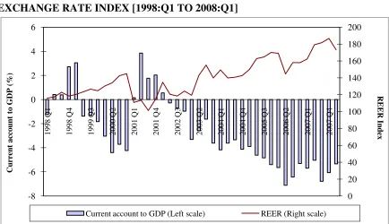
the program and by the late 1990s the current account deficit began deteriorating again (figure

1). This worsening of the current account deficit coincided with an appreciating REER index

(figure 1). As we show later, this appreciation represented an overvaluation in that period.

Excessive dependence on short-term capital flows to finance these deficits put increasing

pressure on the banking sector and by early 2001 Turkey was once again in the midst of a crisis.

FIGURE 1: TURKISH CURRENT ACCOUNT TO GDP AND REAL EFFECTIVE EXCHANGE RATE INDEX [1998:Q1 TO 2008:Q1]

0 20 40 60 80 100 120 140 160 180 200 -8 -6 -4 -2 0 2 4 6 19 98 Q1 19 98 Q4 19 99 Q3 20 00 Q2 20 01 Q1 20 01 Q4 20 02 Q3 20 03 Q2 20 04 Q1 20 04 Q4 20 05 Q3 20 06 Q2 20 07 Q 1 20 07 Q4 REER In d ex Cu rr en t a cc o u n t to G DP (% )

Current account to GDP (Left scale) REER (Right scale)

Notes: The GDP series was expressed in current Turkish lira and the current account series in U.S. dollars. The latter was converted to Turkish lira (using the indicator selling nominal exchange rate).From this we get the ratio of current account to GDP in percentage form. The real effective exchange rate (REER) index is calculated by the IMF as the geometric weighted average of the Turkish price index relative to the price of its trading partners. We use the CPI based index which includes 19 countries including Austria, Belgium, Brazil, Canada, China, France, Germany, Greece, Iran, Italy, Japan, Netherlands, South Korea, Spain, Sweden, Switzerland, Taiwan, U.K. and U.S.A. The base year for the series is 1995. An increase in the index indicates an appreciation. Both series are seasonally adjusted.

The 2001 crisis led to several policy reforms such as the focus on reduced budget deficits,

improvements in the banking sector and a switch to a floating exchange rate regime. There have

been some improvements in Turkey’s external position.3_{Since 2004, Turkey’s export to GDP}

ratio has been high (30%) and increasing. Also, the composition of the current account deficit in

the mid-2000s differs from the period prior to the earlier crisis. The ratio of short term inflows to

the deficit improved (declining to 18% from much higher levels in earlier periods) and there was

an increase in both foreign direct investment as well as long term capital flows. In fact, Turkey’s

reserves increased significantly in the 2000s because of large capital inflows. Towards the end of

the decade, Turkey was also able to make debt payments to the IMF which signaled improved

conditions despite the high levels of deficit.

However, despite these improvements, the overall current account deficit has continued to

mount. Figure 1 shows a sharply deteriorating current account deficit from 2004 onwards. This

increase in deficits coincides with a major appreciation in the REER index and led to fears of an

overvalued lira and the potential for another crisis. However, as noted earlier appreciation does

not necessarily indicate an overvalued currency. And there are reasons to question if the lira is so

significantly overvalued to contribute to these large current account deficits or in fact, if the lira

is overvalued at all. As the literature notes, overvaluation is a lesser concern in floating exchange

rate regimes. Also, changed conditions (discussed above) have an effect on the equilibrium real

exchange rate which may necessitate an appreciation. To more carefully explore the concerns

with the lira, we first need to determine the equilibrium exchange rate and then compare it with

the actual real exchange rate. We present the theoretical and empirical methodology for

equilibrium real exchange rate determination in the next section and estimate it in the following

one.

III. METHODOLOGY

We use Edwards (1989) theoretical framework and cointegration and the error correction

model to estimate the equilibrium real exchange rate for Turkey which is discussed in the

following sub-sections.

A. Theoretical framework

Edwards’ (1989) model defines the real exchange rate as the ratio of the prices of traded to

nontraded goods. The model extended by Elbadawi (1994) examines the impact of various

fundamentals on the price of nontraded goods and thus on the real exchange rate. Any factor that

causes the price of nontraded goods to change will result in a real exchange rate appreciation or

depreciation. Factors that determine the exchange rate are given in the equation below

t t t

t t

t t

t

t tot tariff gcons inv kflows roi tech

e 0 1 2 3 4 5 6 7  (1)

where e is the real exchange rate, tot is terms of trade, tariff is the tariff rate, gcons is

government consumption, inv is investment, kflows is capital flows, roi is the world rate of

interest and tech is technological progress.

Several of these variables have an ambiguous effect. Terms of trade changes can have a

direct income effect (related to demand for nontradables) as well as an indirect substitution effect

(related to supply of nontradables). An improvement in the terms of trade could lead to an

increase in income which by raising demand and thus prices may result in a real exchange rate

appreciation. However, an improvement in terms of trade may also result in increased resources

for producers and thus increased production of all goods (including nontradables). Higher

production can lead to a decline in prices and thus a real exchange rate depreciation.

An increase in tariffrates has two impacts. By raising the domestic price of imports, higher

tariff also leads to a substitution of demand toward domestic goods (including nontraded goods)

which causes an increase in the price of nontraded goods and thus an appreciation.

The impact of investment on the real exchange rate depends on whether higher investment

leads to greater spending on traded goods or toward nontraded goods. Increased spending of the

former implies that higher investment leads to a depreciation of the real exchange rate while

greater spending on nontraded goods leads to an appreciation. Similarly, increased government

consumption directed towards nontraded goods would lead to an appreciation and if it is more

geared toward traded goods we expect a depreciation. Although, this relation is theoretically

ambiguous, the former scenario is more likely.

Capital flows are associated with real exchange rate appreciation. Higher capital inflows

imply greater total assets, which increases general demand (including demand for nontraded

goods). Therefore the price of nontraded goods increases, which results in an appreciation of the

real exchange rate. For similar reasons Alper and Saglam (1999) argue that a fall in the world

rate of interest would result in an appreciation of the real exchange rate. A decline in the world

rate of interest for a debtor country like Turkey would reduce net foreign outflows which leads to

increasing demand for all goods and thus raises the price of nontraded goods leading to a real

exchange rate appreciation.

Finally, technological progress (like terms of trade) can lead to an appreciation if the

increase in assets causes an increase in demand for all goods including nontraded goods. If

instead technological progress leads to increasing production capabilities and thus a decline in

the cost of production, prices of all goods (including nontraded goods) will fall and thus cause a

depreciation.

B. Econometric methodology

We follow the econometric techniques used by the literature in determining the equilibrium

real exchange rate. The first step when dealing with macroeconomic time series described above

is to test for nonstationarity. We use several tests including the Augmented Dickey Fuller (ADF)

test, the Phillips-Perron test, the Kwiatowski, Phillips, Schmidt and Shin (KPSS) test and the

Zivot-Andrews test for determining unit roots in our series.

Nonstationarity implies that standard econometric techniques cannot be used. However, if

these nonstationary series are cointegrated we can use the Error Correction Model (ECM) to

determine the equilibrium real exchange rate. To test for cointegration we first determine the

correct lag length in the VAR (using AIC), then test residuals for normality and serial correlation

and heteroskedasticity. If residuals reveal no problem we test for cointegration using the

Johansen procedure.

If the series are cointegrated the equilibrium real exchange rate is determined using ECM.

The ECM includes nonstationary variables that are cointegrated (long-run determinants) and the

stationary variables (short-run factors) that have an impact on the equilibrium real exchange rate.

Once the ECM is estimated, we test the residuals for stationarity and if stationary, the

coefficients of the cointegrated variables can be used to compute the equilibrium real exchange

rate. Following MacDonald and Ricci (2003), Eita and Sichei (2006), Zalduendo (2006) and

Iossifov and Loukoianova (2007) we use the Hodrick-Prescott filter to capture the permanent

component of this series which gives us our equilibrium real exchange rate.

Through the ECM we determine the speed of adjustment parameters and thus the time it

takes for the deviation in the real exchange rate to be eliminated. The next section describes the

IV. EQUILIBRIUM REAL EXCHANGE RATE ESTIMATION

We use quarterly data from 1998 to 2008 to estimate the equilibrium real exchange rate for

Turkey based on variables in equation (1). We use two measures for the exchange rate. 4 They

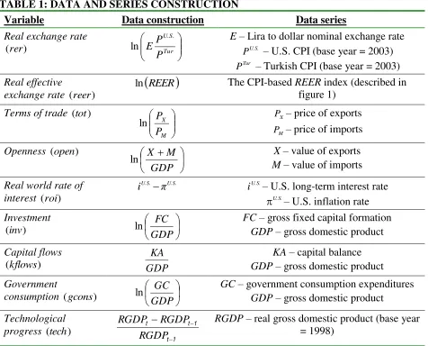
are described in table 1 with other variables used in the estimation.

TABLE 1: DATA AND SERIES CONSTRUCTION

Variable Data construction Data series

Real exchange rate )

(rer 

     Tur U.S. P P E

ln E– Lira to dollar nominal exchange rate U.S.

P – U.S. CPI (base year = 2003)

Tur

P – Turkish CPI (base year = 2003)

Real effective

exchange rate (reer)





ln The CPI-based REER index (described in

figure 1)

Terms of trade (tot)

      M X P P

ln PX – price of exports

M

P – price of imports

Openness (open)

       GDP M X

ln X– value of exports

M– value of imports

Real world rate of

interest (roi)

U.S. U.S. π

i  U.S.

i – U.S. long-term interest rate U.S.

 – U.S. inflation rate

Investment )

(inv _

    GDP FC

ln FC– gross fixed capital formation

GDP– gross domestic product

Capital flows )

(kflows _GDP

KA KA– capital balance GDP– gross domestic product

Government

consumption (gcons) _

    GDP GC

ln GC– government consumption expenditures

GDP– gross domestic product

Technological

progress (tech)

1 t 1 t t    RGDP RGDP

RGDP RGDP– real gross domestic product (base year

= 1998)

Notes: Quarterly data from 1998:Q1 to 2008:Q1 is used. Data for GDP, investment and nominal exchange rate came from Central Bank of Turkey and the rest from International Financial Statistics database. All series are seasonally adjusted using the X11 additive method.

An increase indicates a depreciation in rerand an appreciation inreer. Due to lack of data

we use openness as a proxy for tariff rates. In addition to these factors we add a dummy variable

to capture the change in the exchange rate regime (denoted as derr) after the 2001 crisis. Based on

the econometric techniques described earlier, the above data is used to estimate the equilibrium real exchange rate.

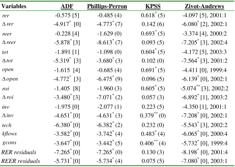
The first task is to test our series for unit roots which are reported in table 2.

TABLE 2: UNIT ROOT TESTS

Variables ADF Phillips-Perron KPSS Zivot-Andrews

rer -0.575 [5] -0.485 (4) 0.618* (5) -4.097 [5], 2001:1

rer

 -4.917* [0] -4.773* (7) 0.142 (6) -6.080* [2], 2002:1 reer -0.228 [4] -1.629 (0) 0.693* (5) -3.374 [4], 2000:2

reer

 -5.878* [3] -8.613* (7) 0.093 (5) -7.205* [3], 2002:4 tot -1.891 [1] -1.098 (0) 0.604* (5) -4.172 [5], 2003:3

tot

 -5.319* [3] -3.680* (3) 0.102 (0) -7.564* [3], 2001:2 open _{-1.615 [4] -0.685 (4) 0.691}* _{(5) -4.411 [0], 1999:4}

open

 -4.772* [3] -6.475* (9) 0.096 (5) -6.139* [0], 2002:1 roi -1.405 [8] -1.960 (3) 0.605* (5) -5.074** [3], 2002:2

roi

 -3.480* [3] -7.071* (2) 0.057 (3) -6.892* [1], 2003:2 inv -1.975 [0] -2.077 (1) 0.223 (5) -4.350 [1], 2001:1

inv

 -4.651* [0] -4.631* (3) 0.379** (0) -7.208* [0], 2002:1 tech -6.380* [0] -6.382* (2) 0.232 (0) -5.543* [3], 2002:2

kflows -3.582* [0] -3.742* (4) 0.483* (4) -6.065* [0], 2000:4

gcons _-3.647* _{[0] -3.442}* _{(5) 0.406}** _{(4) -5.732}* _{[0], 1999:4}

RER residuals -7.265* [0] -7.265* (0) 0.130 (3) -8.198* [0], 2001:4

REER residuals -5.731* [0] -5.734* (4) 0.075 (5) -7.080* [0], 2003:1

Notes: * and ** indicate statistical significance at the 5% and 10% respectively. All tests are

conducted assuming a constant. Tests based on no constant or a constant and trend (not reported here but available on request) have similar conclusions. The null hypothesis for all tests except the KPSS test is that the series is nonstationary. Numbers in square brackets following the ADF and ZA tests correspond to lags where maximum lags were set at 9 and lag length was

determined by AIC. The structural break periods for the ZA test are also reported. For the PP and KPSS tests, the numbers in brackets correspond to lag truncation determined by Newey-West criteria and Schwert formula respectively.

We find that the real exchange rate (both measures), terms of trade, openness, investment and

world rate of interest are nonstationary while capital flows, government consumption and

Before we estimate the error correction models (referred to as RERand REER models) we

test for cointegration between the nonstationary variables. Based on AIC we find the appropriate

lag length for the underlying VAR to be 2 lags. Diagnostic tests (normality, homoskedasticity

and no serial correlation) are conducted on the residuals and the results are reported in table 3.

Except for skewness in the RER model, there are no significant problems of non-normality, serial

correlation or heteroskedasticity in the results. Thus, we can use the Johansen test for

cointegration.

TABLE 3: DIAGNOSTIC TEST RESULTS

RER model REER model

Test Test statistic p-value Test statistic p-value

Serial correlation (LM statistic) 17.828 0.850 14.096 0.960

White heteroskedasticity test

 

 

 

use the White heteroskedasticity test with no cross terms. ** indicates rejection of the null

hypothesis at 10% level of significance.

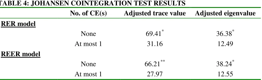
The cointegration test is conducted assuming a constant and no trend in the cointegrating

equation. There is a concern (noted in the literature) of false rejection of no cointegration in

small samples. To remedy this, we follow Baharumshah, Lau and Fountas (2003) in using the

Reinsel and Ahn (1988) correction method and these adjusted results are reported in table 4. We

find evidence of one cointegrating relation for both models. We also perform a chi-square test

for exclusion of each variable. Results (not reported) show that all variables should be included

long-run (nonstationary cointegrated variables) and the short-long-run determinants (stationary variables

and the exchange rate regime dummy variable).

TABLE 4: JOHANSEN COINTEGRATION TEST RESULTS

No. of CE(s) Adjusted trace value Adjusted eigenvalue

RER model

None 69.41* 36.38*

At most 1 31.16 12.49

REER model

None 66.21** 38.24*

At most 1 27.97 12.55

Notes: * and ** denotes rejection of the null of no cointegration at 5% and 10% level of

significance respectively. Adjusted values are computed by multiplying the Johansen test statistics with the small-sample correction factor noted in Reinsel and Ahn (1988). The

correction factor is





the number of lags.

Unit root tests on the residuals of ECM (reported in table 2) show that the residuals are

stationary. Thus we can use the ECM results which are reported in table 5.

We find terms of trade to be negatively associated with rerand reer. As discussed earlier,

terms of trade has a theoretically ambiguous relationship. Our results for the RERmodel show

that an improvement in the terms of trade results in a real exchange rate appreciation while we

get the opposite result for the REER model. This implies that the direct (income) effect of a terms

of trade improvement dominates the indirect (substitution) effect for rerand the reverse is true

for reer. Interestingly this result in theRERmodel is similar to Alper and Saglam (1999) who use

the same measure of the real exchange rate while the REER model results are similar to Atasoy

and Saxena (2006) who use reer in their estimation. This variable is statistically significant at 5%

for the REER model. However, it is only statistically significant at 15% for the RER model.

A higher level of openness (which corresponds to lower tariffs in the model) results in an

several researchers have found that increased openness results in a depreciation of the real

exchange rate. Our findings contradict the expected results. The variable is statistically

significant in both models.

TABLE 5: ERROR CORRECTION MODEL RESULTS

RER model REER model

Variable Coefficient SE Coefficient SE

tot -0.660** (0.471) -1.172* (0.316)

open _-1.178* _{(0.290) 0.408}* _(0.192)

roi 0.118* (0.024) -0.081* (0.016)

inv -1.033* (0.138) 0.815* (0.094)

constant -3.994 7.015

coint equation -0.242* (0.113) -0.402* (0.186)

constant (VAR) -0.445 1.211

derr 0.049+ (0.044) -0.104* (0.056)

tech -1.068* (0.551) 1.178** (0.798)

kflows -0.159+ (0.196) 0.235+ (0.285)

gcons _-0.208+ _{(0.235) 0.543}* _(0.323)

2

R 0.418 0.295

Notes: * and ** indicates statistical significance at 5% and 10% level of significance. + indicates

that although the variable is not statistically significant, exclusion of it is rejected based on

adjusted R and AIC. 2

The world rate of interest, leads to an expected and statistically significant depreciation of

the currency in the two models. An increase in investment is associated with a statistically

significant appreciation of the exchange rate in both models. This indicates that the increased

investment is associated with higher spending on nontraded goods.

Expectedly, we find that a shift in the exchange rate regime is associated with a depreciation

of the currency. While this variable is not statistically significant in the RERmodel (at usual

levels of significance), exclusion of the variable based on adjusted 2

R and Akaike and Schwarz

criterion is rejected. We find that in both models technological progress results in a statistically

dominates over the supply (increased productivity) effect. If technological progress can be seen

as a proxy for productivity growth then it implies that higher productivity leads to a currency

appreciation (Balassa-Samuelson effect). As expected, increased capital flows and government

consumption both lead to an appreciation of the currency. While these are not statistically

significant variables in theRERmodel exclusion of the variables are rejected.

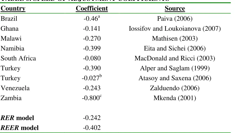
Table 6 reports the speed of adjustment parameters for our two models as well as those

estimated by others for different countries.

TABLE 6: SPEED OF ADJUSTMENT COEFFICIENTS

Country Coefficient Source

Brazil -0.46a Paiva (2006)

Ghana -0.141 Iossifov and Loukoianova (2007)

Malawi -0.270 Mathisen (2003)

Namibia -0.399 Eita and Sichei (2006) South Africa -0.080 MacDonald and Ricci (2003) Turkey -0.390 Alper and Saglam (1999) Turkey -0.027b Atasoy and Saxena (2006)

Venezuela -0.243 Zalduendo (2006)

Zambia -0.800c Mkenda (2001)

RER model -0.242

REER model -0.402

Notes: Annual data was used for Brazil, Namibia, Venezuela and Zambia. Ghana, Malawi,

South Africa and Turkey (both papers) used quarterly data as we did. aPaiva (2006) estimates

four models. We report the coefficient of model 1. bAtasoy and Saxena (2006) estimate five

models. The coefficient reported is that of model 2 which they use as their baseline model.

c

Mkenda (2001) uses three exchange rates for Zambia, one for exports, one for imports and the other an internal real exchange rate. We report the coefficient for the last one.

We find the speed of adjustment parameter to be -0.242 and -0.402 for theRERand

theREERmodel respectively. Our results fall within the estimates seen in the literature. From the

coefficient, following Mathisen (2003) we find that 50% of the deviation in the Turkish rercan

deviation in the real effective exchange rate to be eradicated. This is relatively quick adjustment

similar to Alper and Saglam (1999) for Turkey and Mathisen (2003) for Malawi.

Using the results of the ECM we compute the equilibrium real exchange rate. Following the

literature we use the Hodrick-Prescott filter to remove the cyclical portion so that only the

“permanent” components remain. The actual and the equilibrium real exchange rate are plotted

in figures 2 and 3 for the two exchange rate measures.

FIGURE 2: ACTUAL AND EQUILIBRIUM REAL EXCHANGE RATE [1998:Q2 TO 2008:Q1] 0 0.1 0.2 0.3 0.4 0.5 0.6 0.7 0.8 0.9 19 98 Q2 19 99 Q1 19 99 Q4 20 00 Q3 20 01 Q2 20 02 Q1 20 02 Q4 20 03 Q3 20 04 Q2 20 05 Q1 20 05 Q4 20 06 Q 3 20 07 Q2 20 08 Q1 Lira to d o ll a r ra te

rer erer (Hodrick-Prescott filter)

Source: Central Bank of Turkey and authors’ computation.

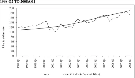
We find that the rer is below and reer is above the respective equilibrium levels prior to the

2001 crisis. This indicates an overvaluation. The next several quarters witness a major

undervaluation in both cases which suggests adjustment in the exchange rate following the crisis

and the reforms undertaken. For the remainder of the sample period the actual real exchange rate

fluctuates around its equilibrium not deviating significantly for a major period of time. We

FIGURE 3: ACTUAL AND EQUILIBRIUM REAL EFFECTIVE EXCHANGE RATE [1998:Q2 TO 2008:Q1]

0 20 40 60 80 100 120 140 160 180 200 19 98 Q2 19 99 Q1 19 99 Q4 20 00 Q3 20 01 Q2 20 02 Q1 20 02 Q4 20 03 Q3 20 04 Q2 20 05 Q1 20 05 Q4 20 06 Q3 20 07 Q2 20 08 Q1 Lira to d o ll a r ra te

reer ereer (Hodrick-Prescott filter)

Source: IMF, International Financial Statistics database and authors’ computation.

V. REAL EXCHANGE RATE MISALIGNMENT

Misalignment is computed as,

ER m Equilibriu ER m Equilibriu ER Actual nt

Misalignme   (2)

Once we compute real exchange rate misalignment we test for a structural break in the series.

This is important given that our sample period includes both a fixed and a floating exchange rate.

Testing and identifying structural breaks allows us to examine if the regimes matter for

misalignment of the real exchange rate. Bai and Perron (1998) propose a procedure for

identifying multiple structural breaks which tests for m structural breaks which indicates m+1

structural regimes. This procedure has been used for examining structural breaks in U.S. inflation

by Jouini and Boutahar (2003) and by Hoarau, Ahamada and Nurbel (2008) for the Australian

We apply the Bai and Perron (1998) procedure on our misalignment series, but constrain the

number of breaks to be no more than two based on our short sample period. We find two

structural breaks using both measures of the real exchange rate. This implies that the

misalignment series can be broken up into three structural regimes which are determined to be

(1) 1998:Q3 to 2000:4, (2) 2001:Q1 to 2002:Q4 and (3) 2003:Q1 to 2008:Q1. The first period

which is prior to 2001 crisis corresponds to a fixed exchange rate regime. The second regime

encompasses the 2001 lira crisis and includes the movement to a floating regime (denoted as the

transitional period). The third regime can be thought of as the post-crisis period covers the period

after Turkey begins recovering from the crisis.The trend in misalignment is seen in figures 2 and

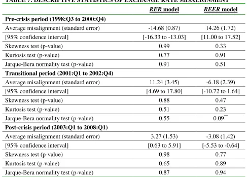
3 and table 7 reports descriptive statistics.

In general, we find that misalignment exhibits no skewness and/or kurtosis and the series is

normal (table 7).5 From figures 2 and 3 we see that lira is consistently overvalued in the

pre-crisis period. In addition, this misalignment is significant with an average overvaluation of

14.68% for rer and 14.26% for reer (table 7). These results confirm findings by Atasoy and

Saxena (2006) of high levels of overvaluation prior to the 2001 crisis. The average misalignment

in the transitional period is in the opposite direction meaning that the real exchange rate is

undervalued on average (11.24% and 6.18% for rer and reer respectively). The third regime has

a lower magnitude of misalignment. However, we find that the lira is undervalued on average

(3.27% and 3.08% for rer and reer respectively). It is likely that this trend is capturing

movement in the world’s major currencies. Thus, it does not provide irrefutable evidence of

undervaluation. However, this is not our focus. Rather, we are arguing that our evidence shows

that the lira is not overvalued in the period following the shift to a floating regime. Overall, our

5 _{One concern is that the Jarque-Bera test for normality is rejected in the REER model at 10% level of significance}

results confirm those of Kemme and Roy (2005), Coudert and Couhard (2008), Holtemöller and

Mallick (2008) and Caputo and Magendzo (2009) that find lower misalignment in more flexible

exchange rate regimes.

TABLE 7: DESCRIPTIVE STATISTICS OF EXCHANGE RATE MISALIGNMENT

RER model REER model

Pre-crisis period (1998:Q3 to 2000:Q4)

Average misalignment (standard error) -14.68 (0.87) 14.26 (1.72) [95% confidence interval] [-16.33 to -13.03] [11.00 to 17.52]

Skewness test (p-value) 0.99 0.33

Kurtosis test (p-value) 0.77 0.91

Jarque-Bera normality test (p-value) 0.91 0.51

Transitional period (2001:Q1 to 2002:Q4)

Average misalignment (standard error) 11.24 (3.45) -6.18 (2.39) [95% confidence interval] [4.69 to 17.80] [-10.72 to 1.64]

Skewness test (p-value) 0.88 0.47

Kurtosis test (p-value) 0.51 0.23

Jarque-Bera normality test (p-value) 0.55 0.09**

Post-crisis period (2003:Q1 to 2008:Q1)

Average misalignment (standard error) 3.27 (1.53) -3.08 (1.42) [95% confidence interval] [0.63 to 5.91] [-5.53 to -0.64]

Skewness test (p-value) 0.98 0.77

Kurtosis test (p-value) 0.65 0.89

Jarque-Bera normality test (p-value) 0.87 0.94

Notes: Using the Bai and Perron (1998) procedure we find two structural break points in the misalignment series and thus three structural regimes noted above. A positive misalignment for rer implies an undervaluation and a positive misalignment for reer implies an overvaluation. Null hypothesis for tests conducted are that there is no skewness, no kurtosis and the series is

normal. ** denotes rejection of the null at 10% level of significance.

The standard deviations of the three regimes show that the greatest volatility is observed in

the transitional period while the other two are more stable with similar levels of standard

deviations (table 7). It is not surprising that we find the transitional period to be highly volatile.

from one exchange rate regime to another. This volatility is reflected in the bigger range of the

95% confidence interval which covers both undervaluation and overvaluation (table 7).

As expected there is less volatility in the post-crisis period compared with the transitional

period. However, we find confirmation for the concern that flexible regimes are more volatile

than fixed regimes. While the standard deviations are similar for the pre-crisis and post-crisis

periods, figures 2 and 3 show that the post-crisis period includes periods of overvaluation and

undervaluation. This reflects volatility in the lira in the post-crisis period which is not captured

by just the standard deviation.

Overall, we find in Turkey’s case that overvaluation of the currency is a significant concern

during a fixed exchange rate regime. Volatility is a bigger concern for floating regimes.

However, it is important to note that the post-crisis period which exhibits volatility in the lira is

not significantly more unstable than the period when Turkey had a fixed exchange rate regime

(pre-crisis period).

VI. CONCLUSION

This paper aims to analyze misalignment of the Turkish lira over different exchange rate

regimes. Using quarterly data from 1998-2008 we employ Edwards (1989) theoretical

framework and cointegration and ECM methodology to compute the equilibrium real exchange

rate and misalignment. In addition, we test for structural breaks in the misalignment series using

the Bai and Perron (1998) procedure and find two breaks which indicate three structural regimes

denoted as pre-crisis period, transitional period and post-crisis period. We analyze misalignment

in these three regimes and as expected, find that on average the lira was significantly overvalued

prior to the 2001 crisis. The transitional period is marked by significant undervaluation and

a floating regime. While the lira is also overvalued in the last period, the magnitude is

significantly lesser than the pre-crisis period. We also find that the post-crisis period is less

volatile than the transitional period, but since it includes both periods of overvaluation and

undervaluation it is more volatile than the pre-crisis period.

Comparing the real exchange rate misalignment to current account deficits in these three

regimes shows that overvaluation was a factor in deteriorating current account deficits in the first

regime (which had a fixed exchange rate). While the real exchange rate has appreciated in recent

years, so have the fundamentals that impact the equilibrium real exchange rate. Thus,

overvaluation is a lesser concern in the latter part of the decade. This means that unlike the

1990s, an overvalued lira is not the contributing factor to exploding current account deficits in

REFERENCES

Alper C. E. and Saglam, I., 1999. The Equilibrium Real Exchange Rate: Evidence from Turkey,

MPRA Working Paper no. 1924.

Atasoy, D. and Saxena, S. C., 2006. Misaligned? Overvalued? The Untold Story of the Turkish

Lira, Emerging Markets Finance and Trade 42, no. 3: 29-45.

Baharumshah, A.Z., Lau, E. and Fountas, S., 2003. On the Sustainability of Current Account

Deficits: Evidence from Four ASEAN Countries, Journal of Asian Economics 14, 465-487.

Bai, J. and Perron, P., 1998. Estimating and Testing Linear Models with Multiple Structural

Changes, Econometrica 66, no. 1: 47-78.

Caputo, R. and Magendzo, I., 2009. Do Exchange Rate Regimes Matter for Inflation and

Exchange Rate Dynamics? The Case of Central America, Central Bank of Chile Working Paper,

June.

Civcir, I., 2003. Before the Fall was the Turkish Lira Overvalued? Eastern European Economics

41, no. 2:69-99.

Coudert, V. and Couhard, C., 2008. Currency Misalignments and Exchange Rate Regimes in

Emerging Markets and Developing Countries, CEPII Working Paper No. 2008-07, April.

Edwards S., 1989. Real Exchange Rates, Devaluation and Adjustment: Exchange Rate Policy in

Developing Countries, Cambridge Massachusetts: MIT Press.

Égert, B. and Lahrèche-Révil, A., 2004. Estimating the Equilibrium Exchange Rate of the

Central and Eastern European Acceding Countries: The Challenge of Euro Adoption, Review of

World Economics 139, no. 4:683-708.

Eita, J.H. and Sichei, M., 2006. Estimating the Equilibrium Real Exchange Rate for Namibia,

Elbadawi, I., 1994. Estimating Equilibrium Long-Run Exchange Rates in Estimating Equilibrium

Exchange Rates, ed. John Williamson, Washington, DC: Institute of International Economics.

Feyzioğlu, T., 1997. Estimating the Equilibrium Real Exchange Rate: An Application to Finland,

IMF Working Paper WP/97/109.

Goldfajn, I. and Valdés, R., 1999. The Aftermath of Appreciations, Quarterly Journal of

Economics 114, no. 1: 229-262.

Hoarau, J.F., Ahamada, I. and Nurbel, A., 2007. Multiple Structural Regimes in Real Exchange

Rate Misalignment: The Case of Australian Dollar, Applied Economics Letters 15, No. 2:

101-104.

Holtemöller, O., and Mallick, S., 2008. Does the Choice of a Currency Regime Explain Real

Exchange Rate Misalignment?, Working Paper, April.

Iossifov, P. and Loukoianova, E., 2007. Estimation of a Behavioral Equilibrium Exchange Rate

Model for Ghana, IMF Working Paper WP/07/155.

Jouini, J. and Boutahar, M., 2003. Structural Breaks in the U.S. Inflation Process: A Further

Investigation, Applied Economics Letters 10, No. 15: 985-988.

Kemme, D. M. and Roy, S., 2005. Real Exchange Rate Misalignment: Prelude to Crisis?”

William Davidson Institute Working Paper No. 797, October.

MacDonald, R., and Ricci, L.A., 2003. Estimation of the Equilibrium Real Exchange Rate for

South Africa, IMF Working Paper WP/03/44.

Mathisen, J., 2003. Estimating the Equilibrium Real Exchange Rate of Malawi, IMF Working

Paper WP/03/104.

Mkenda, B.K., 2001. Long-Run and Short-Run Determinants of the Real Exchange Rate in

Oğuş Binatlı A. and Sohrabji, N., 2008. Analyzing the Present Sustainability of Turkey’s Current

Account Position, Journal of International Trade and Diplomacy 2, No. 2: 171-209.

Paiva, C., 2006. External Adjustment and Equilibrium Exchange Rate in Brazil, IMFWorking

Paper WP/06/221.

Reinsel, G. C. and Ahn, K.S., 1988. Asymptotic Distribution of the Likelihood Ratio Test for

Cointegration in the Nonstationary Vector Autoregressive Model, University of Wisconsin

Madison Working Paper.

Sohrabji, N., 2011. Capital Inflows and Real Exchange Rate Misalignment: The Indian

Experience, Indian Journal of Economics and Business (forthcoming).

Sarno, L., 2000. Real Exchange Rate Behavior in High Inflation Countries: Empirical Evidence

from Turkey, 1980–97, Applied Economics Letters 7, No. 5: 285–291.

Togan, S. and Berument, H., 2007. The Turkish Current Account, Real Exchange Rate and

Sustainability: A Methodological Framework, Journal of International Trade and Diplomacy 1,

No. 1:155-192.

Zalduendo, J., 2006. Determinants of Venezuela’s Equilibrium Real Exchange Rate,IMF