Towards a comprehensive physically based rainfall runoff model

Towards a comprehensive physically-based rainfall-runoff model

Zhiyu Liu and Ezio Todini

Department of Earth and Geo-Environmental Sciences, University of Bologna, Via Zamboni 67, 40127 Bologna, Italy

Email for corresponding author: [email protected]

Abstract

This paper introduces TOPKAPI (TOPographic Kinematic APproximation and Integration), a new physically-based distributed rainfall-runoff model deriving from the integration in space of the kinematic wave model. The TOPKAPI approach transforms the rainfall-rainfall-runoff and runoff routing processes into three ‘structurally-similar’ non-linear reservoir differential equations describing different hydrological and hydraulic processes. The geometry of the catchment is described by a lattice of cells over which the equations are integrated to lead to a cascade of non-linear reservoirs. The parameter values of the TOPKAPI model are shown to be scale independent and obtainable from digital elevation maps, soil maps and vegetation or land use maps in terms of slope, soil permeability, roughness and topology. It can be shown, under simplifying assumptions, that the non-linear reservoirs aggregate into three reservoir cascades at the basin scale representing the soil, the surface and the drainage network, following the topographic and geomorphologic elements of the catchment, with parameter values which can be estimated directly from the small scale ones. The main advantage of this approach lies in its capability of being applied at increasing spatial scales without losing model and parameter physical interpretation. The model is foreseen to be suitable for land-use and climate change impact assessment; for extreme flood analysis, given the possibility of its extension to ungauged catchments; and last but not least as a promising tool for use with General Circulation Models (GCMs). To demonstrate the quality of the comprehensive distributed/ lumped TOPKAPI approach, this paper presents a case study application to the Upper Reno river basin with an area of 1051 km2 _{based on a} DEM grid scale of 200 m. In addition, a real-world case of applying the TOPKAPI model to the Arno river basin, with an area of 8135 km2 and using a DEM grid scale of 1000 m, for the development of the real-time flood forecasting system of the Arno river will be described. The TOPKAPI model results demonstrate good agreement between observed and simulated responses in the two catchments, which encourages further developments of the model.

Keywords: rainfall-runoff modelling, topographic, kinematic wave approximation, spatial integration, physical meaning, non-linear reservoir

model, distributed and lumped

Introduction

The study of the impacts of land use and climate changes on the hydrological regimes of river basins requires a better understanding of how climate, topography-geomorphology, soils and vegetation interact to control runoff at the field, hillslope and catchment scales. These interactions can be represented within complex physically-based distributed models (e.g. SHE: Abbott et al., 1986 a,b). But, traditional physically-based distributed models usually work at a small size and require a large amount of data and lengthy computation times which limit their application. Todini (1988) has pointed out that a promising direction in model development is to lump the differential equations at increasing scales except for a few essential parameters and to make them computationally affordable. Although the validity of effective parameter values that must be used with

large scale catchments has been questioned (Beven, 1989), nonetheless a correct integration of the differential equations from the point to the finite dimension of a pixel, and from the pixel to larger scales, can actually generate relatively scale-independent physically- based models, which preserve the physical meaning (although as averages) of the model parameters.

forecasting. The major disadvantage of the ARNO model is the lack of physical grounds for establishing some of the parameters, which reduces its possible extension to ungauged catchments. The TOPMODEL is a variable contributing area model in which the predominant factors determining the formation of runoff are represented by the topography, the transmissivity of the soil and its vertical delay. However, the model preserves its physical meaning only at the hillslope scale (Franchini et al., 1996), while it degrades into a conceptual model at larger scales, with the same problems mentioned for the ARNO model.

In contrast, the TOPKAPI model is based on the lumping of a kinematic wave assumption in the soil, on the surface and in the drainage network, and leads to transforming the rainfall-runoff and runoff routing processes into three non-linear reservoir differential equations which can be solved analytically (Liu, 2002). The geometry of the catchment is described by a lattice of cells (the pixels of a DEM) over which the equations are integrated to lead to a cascade of non-linear reservoirs. The parameter values of the TOPKAPI model are scale independent and obtainable from a digital elevation map, soil map and vegetation or land-use map in terms of slope, soil permeability, roughness and topology. It can be shown, under simplifying assumptions, that the non-linear cascade aggregates into a unique non-linear reservoir at the basin level, with parameter values that can be estimated directly from the small scale ones without losing physical meaning.

The present paper explains the overall structure and methodology of the TOPKAPI model, the non-linear reservoir equation and its solution technique, the data requirements, and the model calibration procedure. To demonstrate the quality of the TOPKAPI approach, a case study of applying the TOPKAPI model to the Upper Reno river basin is presented, to clarify the data and calibration requirements of the model together with the aggregation capabilities when moving from the distributed to the lumped versions of the TOPKAPI model. A real-world case of applying the TOPKAPI model to the Arno river basin, with an area of 8135 km2 _{and using a DEM grid scale of 1000 m,} for the development of areal-time flood forecasting system for the Arno River is also presented.

Structure and methodology of the

TOPKAPI model

The TOPKAPI is a comprehensive distributed-lumped approach. The distributed TOPKAPI model is used to identify the mechanism governing the dynamics of the saturated area contributing to the surface runoff as a function of the total water storage, thus obtaining a law underpinning

the development of the lumped model.

The model is based on the idea of combining the kinematic approach with the topography of the basin; the latter is described by a Digital Elevation Model (DEM) whose grid size generally increases with the overall dimensions. Each grid cell of the DEM is assigned a value for each of the physical characteristics represented in the model. The flow paths and slopes are evaluated starting from the DEM, according to a neighbourhood relationship based on the principle of minimum energy cost (Band, 1986).

The integration in space of the kinematic wave equations results in three ‘structurally-similar’ non-linear reservoir equations describing different hydrological and hydraulic processes. This lumping is performed on the individual cell of the DEM in the distributed model, while in the lumped model it is performed at the basin level. The equations obtained for the local scale and for the lumped scale are structurally similar; what distinguishes them are the coefficients, which in one case have local significance and, in the other, summarise the local properties in a global manner.

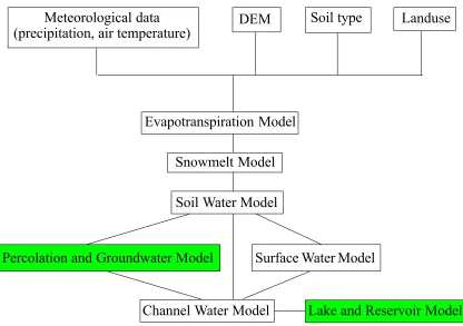
The present TOPKAPI model (Fig. 1) is structured around five modules that represent the evapotranspiration, snowmelt, soil water, surface water and channel water components respectively. For the deep aquifer flow, the response time caused by the vertical transport of water through the thick soil above this aquifer is so large that horizontal flow in the aquifer can be assumed to be almost constant with no significant response on one specific storm event in a catchment (Todini, 1995). Hence, initially, the model does not account for water percolation towards the deeper subsoil layers and for their contribution to the discharge; this is planned as an additional model layer in a future model development.

The soil water component is affected by subsurface flow (or interflow) in a horizontal direction defined as drainage; drainage occurs in a surface soil layer, of limited thickness and with high hydraulic conductivity due to its macro-porosity. The drainage mechanism plays a fundamental role in the model both as a direct contribution to the flow in the drainage network and most of all as a factor regulating the soil water balance, particularly in activating the production of overland flow. The soil water component is the most characterising aspect of the model because it regulates the functioning of the contributing saturated areas. The surface water component is activated on the basis of this mechanism. Lastly, both components contribute to feeding the drainage network.

Fig. 1. The components of the TOPKAPI model

models, e.g. SHE (Abbott et al., 1986 a,b), DHSVM (Wigmosta et al., 1994). However, a simplified approach is generally necessary because in many countries the required historical data for Penman-Monteith estimations are not extensively available; and, in addition, apart from a few meteorological stations, almost nowhere are real-time data available for flood forecasting applications. Evapo-transpiration plays a major role not only in terms of its instantaneous impact, but in terms of its cumulative temporal effect on the soil moisture volume depletion; this reduces the need for an extremely accurate expression, provided that its integral effect is well preserved. In the present TOPKAPI model, evapotranspiration can be introduced directly as an input to the model or computed externally or estimated internally by a radiation method (Doorembos et al., 1984) starting from the temperature and from other topographic, geographic and climatic information, as described in the ARNO model (Todini, 1996). Again, for reasons of limited data availability, the snow accumulation and melting (snowmelt) component is driven by a radiation estimate based upon the air temperature measurements, which is also borrowed from the ARNO model. In the following sections, the three basic components, the soil water, surface water and channel water will be described in detail.

The distributed TOPKAPI model

THE SOIL WATER COMPONENT

Fundamental assumptions

(1) Precipitation is constant over the integration domain (namely the single cell), by means of suitable averaging and lumping operations of the local rainfall data, such as Thiessen polygons and Block Kriging (de Marsily, 1986; Matheron, 1970) techniques;

(2) All of the precipitation falling on the soil infiltrates into it, unless the soil is already saturated in a particular zone; this is equivalent to adopting as the sole mechanism for the formation of overland flow the saturation mechanism from below, (Dunne, 1978);

(3) The slope of the water table coincides with the slope of the ground, unless the latter is very small (less than 0.01%); this constitutes the fundamental assumption of the approximation of the kinematic wave in the Saint Venant equations, and it implies the adoption of a kinematic wave propagation model with regard to horizontal flow, or drainage, in the unsaturated area (Henderson and Wooding, 1965; Beven, 1981); (4) Local transmissivity, like local horizontal flow, depends

on the total water content of the soil, i.e. it depends on

Meteorological data

(precipitation, air temperature)

DEM

Soil type

Landuse

Evapotranspiration Model

Snowmelt Model

Soil Water Model

Surface Water Model

Percolation and Groundwater Model

the integral of the water content profile in a vertical direction;

(5) Saturated hydraulic conductivity is constant with depth in a surface soil layer but is much larger than that at deeper layers; this forms the basis for the vertical aggregation of the transmissivity.

Kinematic wave formulation for sub-surface flow

In the TOPKAPI model, the horizontal sub-surface flow, q, is calculated by the approximation Eqn. (1) (Benning, 1994; Todini and Ciarapica, 2001):

_q=tan

_{( )}

s (1)

with

_∫

_{( )}

_∫

− − = = Θ L r s r L dz L dz z

L _{0 0}

1 ~ 1 ~ ϑ ϑ ϑ ϑ ϑ

where β is the slope angle, k_s is the saturated hydraulic conductivity in ms-1_{, L is the thickness of the surface soil} layer in m, _Θ~ is the reduced soil moisture content, ϑr is

the residual soil moisture content, ϑs is the saturated soil moisture content, ϑ is the water content in the soil, ϑ~( )z is the mean value along the vertical profile of the reduced soil moisture content and α is a parameter which depends on the soil characteristics (Benning, 1994; Todini, 1995).

Combined with the equation for continuity of mass, the following system is obtained:

( ) ( )      Θ = = + Θ − α β ∂ ∂ ∂ ∂ ϑ ϑ ~ tan ~ L k q p x q t L s r s (2)

where x is the main direction of flow along a cell, t is the time, q is the horizontal flow in the soil due to drainage, corresponding to a discharge per unit of width in m2_s–1_{, and} p is the intensity of precipitation in m s–1_{. The model is} written in just one direction since it is assumed that the flow is characterised by a preferential direction, which can be described as the direction of maximum slope.

Equation (2), rewritten in terms of actual total water content in the soil, η=

(

)

( )

(_{ϑ ϑ} )αβ_Lα

Lk C r s s −

= tan (3)

leads to the kinematic equation

( )

(

)

k L p

t _{s r}

s ∂ η ∂ ∂ η ∂ ϑ ϑ β ∂ η

∂ α α

α

α = −

− −

= tan _{. (4)}

Here, the term C represents in physical terms a local conductivity coefficient, since it depends on soil parameters for a particular position or a particular cell, which encompasses the effects of hydraulic conductivity and slope, to which it is directly proportional, and storage capacity, to which it is inversely proportional.

Non-linear reservoir model for the soil water in a generic cell

By integrating Eqn. (4) in the soil over the ith _{DEM grid} cell, whose space dimension is X, gives

(

)

i i s i i i s s s C C pX t

v _{α α}

η η ∂ ∂ 1 1 − − − − = (5)

where vsi is the volume per unit of width stored in the i th

cell in m2_{, while the last term in Eqn. (5) represents the} inflow and outflow balance. A subscript s is introduced here to distinguish this soil water equation from the ones relevant to the overland and the drainage network flows.

It is quite evident that the coefficients C_S are no longer the physically measurable quantities, which are defined at a point; rather, they represent integral average values for the entire cell, which nonetheless are still strongly related to the measurable quantities.

In the TOPKAPI model, the grid cells are connected by a tree shaped network; water moves downslope along this tree-shaped flow pathway starting from the initial cells (without upstream contributing areas) representing the ‘sources’, towards the outlet. According to this procedure, and assuming that in each cell the variation of the vertical water content along the cell is negligible, the volume of water stored in each cell (per unit width) can be related to the total water content that is equivalent to the free water volume in depth, by means of the simple expression

i

i X

v_s = η (6)

Substituting for ηi in Eqn. (6) and writing it for the

“source” cells in each flow pathway, the following non-linear reservoir equation is obtained:

s i s i i s s i s _V X X C X p t V _α α ∂ ∂ 2 2₋

= . (7)

Similarly a non-linear reservoir equation can be written for a generic cell, given the total inflow to the cell, such that

₍

₎

i s i i i i s s u s u o i s V X X C Q Q X p t V _α α ∂ ∂ 2 2 − + + = (8)

( ) p

x q t L

r

s−ϑ ∂_∂Θ+_∂∂ =

ϑ

where

i

s

V is the volume stored in the ith _{cell in m}3_, u oi

Q is the discharge entering the active cell i as overland flow from the upstream contributing area in m3_s–1_{, and} u

si Q _{is the}

discharge entering the active cell as subsurface flow from the upstream contributing area in m3_s–1_.

Soil moisture accounting in a grid cell

For the ith _{cell at each time-step, the soil water balance can}

be calculated as follows:

T t V T t V Q Q X p

Q i i

i i i s s u s u o i d s ) ( ) ( )

( 0 0

'

2_{+ + −} + −

= (9)

(

)

[

]

{

}

max i 0 i 0 i

i s s s

o V t T V t T V

e = + − + (10)

[

]

0

0 ) min '( ),

(t T V t T V E X

Vsi + = si + smi − a (11)

where T is the computational time interval in seconds, t₀ is the initial time of the computation step, (0 )

' _{t T}

V

i

s + is the

solution of Eqn. (8) at the time t₀ + T in m3_{, ( )}

0 t

V_si is the initial soil water storage in the ith_{cell at the time t}

0 in m3 ,

d si

Q _{is the outflow discharge from the i}th_{cell during the time}

t₀ tot₀ + T in m3_s–1_,

i o

e is the saturation excess volume for the ith_{cell in m}3_,

i

sm

V is the saturated soil water storage in the ith_{cell in m}3_{, E}

a is the actual evapotranspiration within

the time interval calculated by the evapotranspiration model in m, and Vsi(t0+T)is the soil water volume stored in the

soil in the ith_{cell at time t} 0 + T.

Up to this point it has been implicitly assumed that the entire outflow from a cell flows into the downstream cell immediately. However, this is not entirely true since note has to be taken of the depletion effected by the drainage network. Thus, for the cells in the channel network, the outflow is still evaluated by Eqn. (9), but it is then partitioned between the channel and the downstream cell according to a gradient based upon the average slope of the four surrounding cells. This allows determination of the amount of subsurface flow feeding the drainage channel network. This operation of flow partition is also performed for the overland flow.

THE SURFACE WATER AND CHANNEL WATER COMPONENTS

The input to the surface water model is the precipitation excess resulting from the saturation of the surface soil layer. In addition, the water in the soil can ex-filtrate on the surface as return flow due to a sudden change in hillslope or soil

property, and thus also feeds the overland flow. The sub-surface flow and the overland flow together feed the channel along the drainage network.

Non-linear reservoir model for overland flow and channel flow in a grid cell

Overland flow routing is described similarly to the soil component, according to the kinematic approach (Wooding, 1965) in which the momentum equation is approximated by means of Manning’s formula. The kinematic wave approximation for overland flow is described as

      = = − = o o o o o o o o o h C h n q x q r t h α β ∂ ∂ ∂ ∂ 3 5 2 1 ) (tan 1 (12)

where h_o is the water depth over the ground surface in m,

o

r is the saturation excess resulting from the solution of the soil water balance, either as the precipitation excess or the ex-filtration from the soil in absence of rainfall in ms-1_,

o

n is the Manning friction coefficient for the surface roughness in _m−13_s−1_,

o

o n

C _=(tanβ)12 _{is the coefficient relevant to}

the Manning formula for overland flow, and αo=53 is the

exponent which derives from using the Manning formula. A subscript o denotes the overland flow.

By analogy with what was done for the soil, assuming that the surface water depth is constant over the cell and integrating the kinematic equation over the longitudinal dimension, gives the non-linear reservoir model for the overland flow for the ith _{cell as}

o i o i i i o o o o V X X C X r t V _α α ∂ ∂ 2 2 ₋ = (13) where Vo_i is the surface water volume in the cell in m3.

Similar considerations also apply to the channel network, which is assumed to be tree-shaped with reaches having wide rectangular cross-sections. In this case, the channel surface width is not constant but is assumed to be increasing towards the catchment outlet. Under these assumptions, the non-linear reservoir model can be written for a generic reach as

(

)

₍

₎

i c i i i c i i i c u c i c c V XW W C Q XW r t V _α α − + = ∂ ∂ ₍₁₄₎

where Vc_iis the volume of water stored in the ith channel

reach in m3_,

i

W is the width of the ith _{rectangular channel}

reach in m, u ci

reaches in m3_s–1_,

c

r is the lateral drainage input, including the overland runoff reaching the channel reach and the soil drainage reaching the channel reach in m s–1_,

c

c s n

C 12 0

=

is the coefficient relevant to the Manning formula for channel flow, s₀ is the bed slope, assumed to be equal to the ground surface slope, nc is the Manning friction coefficient

for the channel roughness in −13 −1

s

m and αc=53 is the exponent which derives from using the Manning formula. The channel width Wi is taken to increase as a function of the area drained by the ith _{cell on the basis of} geomorphological considerations, such that

(

)

th tot

min max max

i A A

A A

W W W

W _i −

    

  

− − +

= (15)

where Wmax is the maximum width, at the basin outlet, Wmin

is the minimum width, corresponding to the threshold area,

Ath is the threshold area which is the minimum upstream

drainage area required to initiate a channel, A_tot is the total area and Adr_i is the area drained by the ith cell.

PHILOSOPHY OF APPLICATION OF THE DISTRIBUTED TOPKAPI MODEL

Solution technique for the non-linear reservoir equation

The TOPKAPI formulation leads to three non-linear reservoir equations describing the subsurface flow, the overland flow and the channel flow. In the first version of the TOPKAPI model (Todini and Ciarapica, 2001), the solution of the non-linear reservoir equation was based upon a variable step fifth order Runge-Kutta numerical algorithm due to Cash and Karp (1990). Nowadays, the authors have found that the non-linear reservoir equation can be solved analytically based on an appropriate approximation (Liu, 2002), providing a more efficient scheme in terms of running time. Details of analytical solutions based on appropriate approximations are given in Appendix A.

Data requirements and parameters

The TOPKAPI model requires terrain data (e.g. from DTM or DEM land survey), soil survey and vegetation or land-use, as well as geographical co-ordinates and measurements of precipitation, evapotranspiration or air temperature.

As far as the parameters are concerned, there are seven classes of parameters in the TOPKAPI model, namely L (thickness of the surface soil layer in m), k_s (saturated hydraulic conductivity in m s–1_{),ϑr (residual soil moisture} content),ϑs(saturated soil moisture content), a_s(exponent

of the transmissivity law for the soil component, assumed to be constant for all the cells), no(surface roughness in

1 3 1 ₋

−

s

m ), and nc(roughness for the channel in m−13s−1) . Five

of the parameters (L, ks,ϑr,ϑsand as) relate to the soil and

control runoff production, whilst the other two (n_o,nc) are routing parameters.

DEM application in the TOPKAPI model

The DEM application consists of: identifying and correcting sinks and false outlets, identifying the connections among the cells thereby giving the flow pathways, calculating the steepness, and cumulating the drained area for the automatic detection of the drainage network. Utilities serving these purposes are provided in GRASS (Geographic Resources Analysis Support System), but unfortunately they are not suitable for application to the TOPKAPI model because they are based on neighbourhood functions that use a moving 3 × 3 point spatial window, where the elevation of the central point is compared with the heights of the eight connected neighbours. For the TOPKAPI model, or in general for any model using a finite difference approach, in the moving 3 × 3 point spatial window the four neighbouring cells adjacent to each corner have to be neglected, which means physically that drainage is only possible to the north, east, south or west for the four adjacent cells at each edge.

Model calibration

The TOPKAPI model is considered as a physically based model, with all parameters having physical meanings which can be measured directly through fieldwork. Although it is physically based, the model still needs calibration because of the uncertainty of the information on the topography, soil characteristics and land cover. Nonetheless the calibration of the TOPKAPI parameters is more an adjustment than a conventional calibration and is carried out by a simple trial-and-error method.

Model parameter values are assigned according to the type of soil, land cover and channel order by the method of Strahler (1957). The initial parameter values can be taken from the literature, e.g. the values of the soil parameters ks,

ϑr and ϑs can be taken from the USDA parameters for the infiltration model of Green-Ampt. Initial values for parameters n_o and n_c can be estimated by referring to Tables 5.5 and 5.6 in the book on Open Channel Hydraulics by Chow (1959) and the report on Roughness Characteristics of Natural Channels by Barnes (1967), while a_susually varies 2.0 ~ 4.0 based on the soil property. In general, the ranges of the values of the model parameter are: L=0.10 ~2.00 m, ks= 10-6 ~ 10–3 m s–1, ϑs= 0.25~0.70, ϑr= 0.01~0.10,no= 0.05~0.40 m–1/3 s–1, nc=0.02~0.08 m–1/3 s–1.

The lumped TOPKAPI model

DESCRIPTION OF THE LUMPED TOPKAPI MODEL

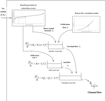
The overall structure of the lumped TOPKAPI model is shown schematically in Fig. 2. A catchment is regarded as a dynamic system composed of three reservoirs: the soil

reservoir, the surface reservoir and the channel reservoir. In the flow simulation, on the basis of the soil condition and actual evapotranspiration, the precipitation in the catchment is partitioned into direct runoff and infiltration using the Beta-distribution curve, which reflects the non-linear relationship between the soil water storage and the saturated contributing area in the basin. The infiltration and direct runoff are input into the soil reservoir and surface reservoir, respectively. Outflows from the two reservoirs as interflow and overland flow are then drained into the channel reservoir to form the channel flow.

As mentioned before, the TOPKAPI approach is a comprehensive distributed-lumped approach. Theoretically it proves that the lumped version of the TOPKAPI model can be derived directly from the results of the distributed version and does not require additional calibration.

In order to obtain the lumped version of the TOPKAPI, the point kinematic wave equation is integrated over the entire system of cells describing the basin. This is done first by computing the total volume stored in the soil, on the surface or in the channel network by adding up the single cell volumes as a function of the geomorphology and

o oT

V b A R R t V

o r d

oT_{= + −} α

∂

∂ _{( )}

S

sT s sT _{RA bV}

t

V _{= −} α

∂ ∂

c

cT c s o

cT _{Q Q bV}

t

V _{= + −} α

∂

∂ _{( )}

Runoff generation by saturation-excesss

Return flow calculation model

S

Suurrffaacceerreesseerrvvooiirr

S Sooiillrreesseerrvvooiir r

C

Chhaannnneellrreesseerrvvooiirr Intteerrffllooww

Qs O

OvveerrllaannddfflloowwQo E

Exxffiillttrraattiioonn

Rate Rr D

Diirreeccttrruunnooffff

Intensity Rd

Infiltration

rate R

C

Chhaannnneellffllooww

Net rainfall

(P-Ea)

topology of the catchment. Under the assumption that the difference between the inflow to a cell and the time variation of the water storage do not vary significantly in space, this integration and aggregation results in a non-linear reservoir equation for representing the basin as a whole of the form (Todini and Ciarapica, 2001; Liu, 2002).

(16)

with

where i is the index of a generic cell, j is the index of cells drained by the ith _{cell, N is the total number of cells in the}

upstream contributing area, VsTis the water storage in the catchment in m3_{, R is the infiltration rate in m s}–1_{, A is the} catchment area,

i

s

C is the local conveyance for the ith _cell,

f_m represents the fraction of the total outflow from the mth

cell which flows towards the downstream cell, αs is a soil

model parameter assumed constant in the catchment, and

s

b is a lumped soil reservoir parameter which incorporates in an aggregated way the topography and physical properties of the soil.

Equation (16) corresponds to a non-linear reservoir model and represents the lumped dynamics of the water stored in the soil. The same type of equation can be written for the overland flow and for the drainage network, thus transforming the distributed TOPKAPI model into a lumped model characterised by three ‘structurally similar’ non-linear reservoirs, namely ‘soil reservoir’, ‘surface reservoir’ and ‘channel reservoir’.

The infiltration rate term in Eqn. (16) must be evaluated by separating precipitation into direct runoff and infiltration into the soil. In order to obtain this separation, a relationship between the extent of saturated areas and the volume stored

in the catchment is introduced, similar to what is done in the Xinanjiang model (Zhao, 1977), in the Probability Distributed Model (Moore and Clarke, 1981; Moore, 1985, 1999) and in the ARNO model (Todini, 1996). Given the availability of the distributed TOPKAPI version, this relationship can be obtained by means of extensive simulation. At each time step the number of saturated cells is compared to the total volume of water stored in the soil over the entire catchment. Denoting total water storage in the soil by V_sT, the soil water storage at the total saturation

condition by Vss, and the total saturation area by As, the

relationship between the extent of saturated areas and the volume stored in the catchment can be approximated by a Beta-distribution function curve expressed by:

(17)

where Γ(⋅)is the Gamma function, and r and s two parameters of the Beta-distribution curve.

Surface runoff calculation

Surface runoff is the sum of direct runoff and the return flow caused by ex-filtration. In the lumped TOPKAPI model, the Beta-distribution function curve as expressed by Eqn. (17) is thus used to compute, in the lumped form, the overall inflow as infiltration R to the soil reservoir and the overall saturation excess as direct runoff R_d(ms-1_{) entered} into the surface reservoir by the following equation:

)

(_{2 1}

1 2 t t A V V V V V P R ss ss sT ss sT d −     − − = ₍₁₈₎

where VsT₁, VsT₂ represent the soil water storage in the

catchment at time t₁, and t₂=t₁+∆t respectively where ∆t is the computation time interval, and P represents the catchment average net precipitation intensity (m s-1_).

The soil water can ex-filtrate to generate the return flow. In the present TOPKAPI model, the return flow is estimated based on a limiting parabolic curve representing the relationship between the return flow discharge and the fraction of water storage in the catchment, which is estimated based on the points from the distributed TOPKAPI model. This parabolic curve can be expressed as:

A a V V A a V V A a A Q R ss sT ss sT return

r 2 3

2

1 _{+ +}

    = = (19) ϕ ϕ ϕ d s r s r A

A r s

V V s ss sT 1 1 0 ) 1 ( ) ( ) ( ) ( _{− −} − Γ Γ + Γ =

_∫

∑ ∏

∑ ∏

f

f

C

































−





































+









+

=

∑

∑ ∏

∑ ∏

1

1

sTV RA bV

C

X α = − α

where R_ris the return flow ex-filtration rate, Qreturn is the

calculated return flow discharge on the surface during the time interval t₁ ~ t₂, V_sT =0.5(V_sT1+V_sT2) is the averaged soil water storage in m3_{, and a}

1, a2 and a3are parameters

estimated on the basis of the points from the distributed TOPKAPI model.

Accordingly, the infiltration rate into the soil within the time interval Dt can be computed by:

A Q t t A

V V

V V V

R ss return

ss sT

ss sT

− −   

 − =

) (_{2 1}

1

2 (20)

The quantities R and R_d plus R_r are then input to the soil reservoir and the surface reservoir, respectively (see Fig. 3). The interflow and overland flow can be obtained by computing the water balance, and are then together drained into the channel reservoir to generate the total outflow at the basin outlet.

Fields of application

Since its advent in 1995, the TOPKAPI model has been applied to several catchments for different uses such as flood forecasting, extreme flood analysis, and predicting hydrological response under changed landscape conditions caused by human activities. The distributed version of the TOPKAPI model allows for its calibration on the basis of physical considerations and, in particular, its extension to ungauged catchments. The lumped version of the TOPKAPI model allows for the extensive simulations needed when used in combination with a stochastic rainfall generator for deriving, through continuous simulation, extreme discharges and flood wave volumes.

The model has been applied to the upper Reno river basin (1051 km2_{) (Todini and Ciarapica, 2001) and the Arno river} basin (8135 km2_{) for flood forecasting (Liu, 2002), and to} the Magra catchment (1682 km2_{) for extreme flood analysis} (Liu and Todini, 2000). The DEM grid size employed

0 50 100 150 200 250 300 350 400

90/02/01 07:00 90/02/04 19:00 90/02/08 07:00 90/02/11 19:00 90/02/15 07:00 90/02/18 19:00 90/02/22 07:00 90/02/25 19:00 90/03/01 07:00 90/03/04 19:00 90/03/08 07:00 90/03/11 19:00 90/03/15 07:00 90/03/18 19:00 90/03/22 07:00 90/03/25 19:00 90/03/29 07:00 90/04/01 19:00 90/04/05 07:00 90/04/08 19:00 90/04/12 07:00 90/04/15 19:00 90/04/19 07:00 90/04/22 19:00 90/04/26 07:00 90/04/29 19:00 90/05/03 07:00 90/05/06 19:00 90/05/10 07:00 90/05/13 19:00 90/05/17 07:00 90/05/20 19:00 90/05/24 07:00 90/05/27 19:00 90/05/31 07:00 Time

Discharge (m

3s -1)

Observed Modelled

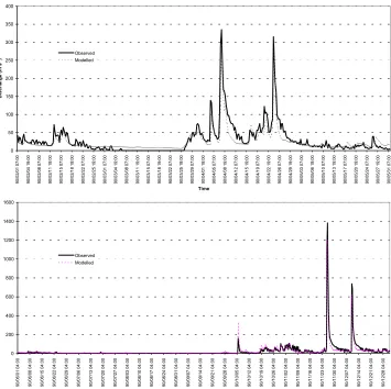
Fig. 3. TOPKAPI model results in the Upper Reno catchment: (a) small flood events, (b) major flood events

0 200 400 600 800 1000 1200 1400 1600

90/06/01 04:00 90/06/08 04:00 90/06/15 04:00 90/06/22 04:00 90/06/29 04:00 90/07/06 04:00 90/07/13 04:00 90/07/20 04:00 90/07/27 04:00 90/08/03 04:00 90/08/10 04:00 90/08/17 04:00 90/08/24 04:00 90/08/31 04:00 90/09/07 04:00 90/09/14 04:00 90/09/21 04:00 90/09/28 04:00 90/10/05 04:00 90/10/12 04:00 90/10/19 04:00 90/10/26 04:00 90/11/02 04:00 90/11/09 04:00 90/11/16 04:00 90/11/23 04:00 90/11/30 04:00 90/12/07 04:00 90/12/14 04:00 90/12/21 04:00 90/12/28 04:00 Time

Discharge (m

3s -1)

increases with the catchment size, ranging from 200 m to 1 km for these three examples.

A case study applying both the distributed and lumped TOPKAPI model to the upper Reno river basin and including the distributed TOPKAPI model for developing a real-time flood forecasting system for the Arno River is presented here in detail.

The Upper Reno river basin case

study

CATCHMENT CHARACTERISTICS

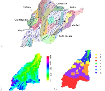
Topography

The Reno River in Italy rises on the northern slopes of the Apennines and flows inside the Emilia-Romagna region (Fig. 4a) with a total watercourse of 210 km. The basin has a surface area of 4930 km2 _{and a variation in height above} sea level of up to 2,000 m (see Fig. 4b). The upper part of the basin is gauged at Casalecchio on the outskirts of the city of Bologna, and drains an area of approximately 1051 km2 _{within which it reaches its maximum elevation of} 2000 m. A digital elevation model (DEM) on a 400 × 400 m

grid is available for most of the Upper Reno river basin falling under the Emilia Romagna Regional Authority.

Soils

The Upper Reno river basin comprises primarily clayey and marly soil, as well as alluvial deposits in its lower section (see Fig. 4c and Table 1).

Table 1. Soil types in the Upper Reno river basin(Fig. 3c)

Class Soil Types

a Arenaceous turbidites, calcarenites

b Arenaceous turbidites, marly limestone turbidites c Marly arenaceous turbidites

d Arenaceous turbidites

e Marly limestone and calcarenite turbidites, clays and marly limestones

f Clays, sands and conglomerates g Alluvial deposits

a)

b)c)

c)

b)

Casalecchio

Vergato Calcara

Castenaso

Mordano Bastia

Sesto Imolese

Vegetation and land use

Vegetation on the highest parts of the Apennines is made up of herbaceous formations and blueberry derived from cultivation and grazing which were once particularly intensive. The most widespread land use in the strip of territory along the Reno, both for the lowland area as well as for the mountain area, is agriculture, except for the impracticable areas at high levels and those areas subject to periodical flooding.

MODEL CALIBRATION OF THE DISTRIBUTED TOPKAPI MODEL

Hydrometerological data availability

The hydrological dataset in the year 1990 is selected for calibration in the Upper Reno river basin, since in this year, from 24 to 26 November, 1990, a relatively large flood event with a peak discharge of 1317 m3_s–1 _{occurred. Hourly} measurements from 24 raingauges and 10 thermometers were available while discharges were computed from hourly levels by means of a well-verified rating curve available for Casalecchio. The areal rainfall distribution was estimated by the Thiessen Polygon method.

Model calibration

The model calibration was performed at a 1-hour time-step using the hydrological dataset of 1990. An initial estimate for the model parameter set was derived using the available broad descriptions of soil types given in Table 1 and Strahler channel order, together with values taken from the literature. Adjustment of parameters was performed manually and, at the end, the values given in Table 2 were retained. The model results are shown in Fig. 3, and the model efficiencies are: 0.850 (R2_{: the proportion of the variance in the observations}

accounted for by the model), 0.843 (r2_{: the coefficient of} determination) and 0.918 (r: the correlation coefficient), respectively.

DERIVATION OF THE LUMPED TOPKAPI MODEL PARAMETERS AND MODEL APPLICATION

As explained previously, the lumped TOPKAPI model can be derived directly from the distributed results of the distributed TOPKAPI model. Given the availability of the distributed TOPKAPI version, at each step in time the number of saturated cells is compared with the total volume of water stored in the soil over the entire catchment. The relationship between the extent of saturated areas and the volume stored in the catchment can be approximated by a Beta-distribution function curve which is shown in Fig. 5. In addition, the distributed TOPKAPI model showed that the overland flow comprises two parts, one from direct runoff in the saturated area and the other from return flow which is the ex-filtration of soil water into the surface. In the Upper Reno river basin, the maximum discharge value of the return flow was 43 m3_s–1_{. Hence, the generation of} return flow is very significant in the catchment, and therefore should be simulated in the lumped TOPKAPI model. Figure 6 shows the relationship between the return flow discharge and the soil water storage in the catchment, and its approximation by the limiting parabolic curve adopted in the lumped TOPKAPI model.

The parameters of the lumped TOPKAPI model are listed in Table 3 and simulation results are shown in Figs. 7 and 8. Figure 7 compares the runoff calculated by the distributed TOPKAPI model with that obtained using the lumped model, while Fig. 8 shows the comparison of the observed discharges at Casalecchio and those computed using the distributed and lumped TOPKAPI model. The lumped TOPKAPI model performance measures are as high as the distributed ones, namely R2 _{= 0.887, r}2 _{= 0.867 and r= 0.931.}

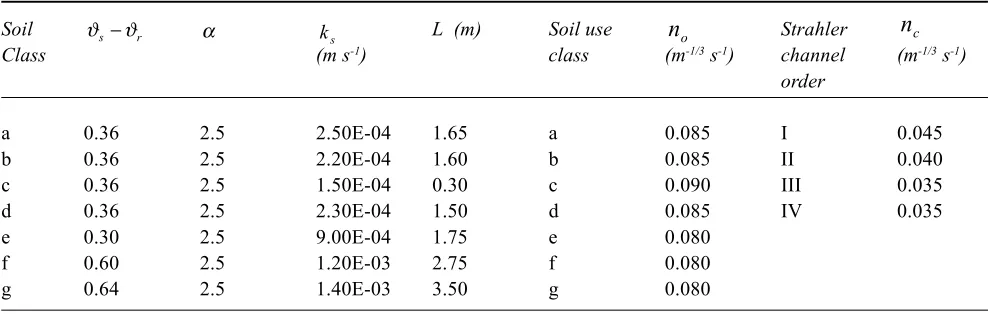
Table 2. Calibration parameters for the different soil classes, land uses and channel orders

Soil ϑs−ϑr α ks L (m) Soil use

n

n

Class (m s-1_{) class (m}-1/3 _s-1_{) channel (m}-1/3 _s-1₎

order

a 0.36 2.5 2.50E-04 1.65 a 0.085 I 0.045

b 0.36 2.5 2.20E-04 1.60 b 0.085 II 0.040

c 0.36 2.5 1.50E-04 0.30 c 0.090 III 0.035

d 0.36 2.5 2.30E-04 1.50 d 0.085 IV 0.035

e 0.30 2.5 9.00E-04 1.75 e 0.080

f 0.60 2.5 1.20E-03 2.75 f 0.080

0 0.1 0.2 0.3 0.4 0.5 0.6 0.7 0.8 0.9 1

0 0.1 0.2 0.3 0.4 0.5 0.6 0.7 0.8 0.9 1

fraction of saturation area (As/A)

fraction of water storage (VsT/VSS)

distributed points beta curve

0 10 20 30 40 50

0.3 0.35 0.4 0.45 0.5 0.55 0.6 0.65 0.7

fracti o n o f w ater sto rag e (VsT /Vss)

Return flow (m3/s)

p arab olic curve

p oints from the d istrib u ted T O P K A P I m od el

R

et

u

rn

fl

o

w (m

3s -1)

Fig. 5. The Beta-distribution function fitted to the distributed TOPKAPI simulated results (r=0.11,s=0.16)

Fig. 6. A limiting parabolic curve used for calculating the return flow from the soil water storage in the catchment (

3 2

2

1 a

V V a V

V a Q

ss sT ss

sT

return =   + +

with a₁=441, a₂=-330, a₃=66.)

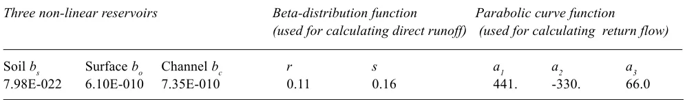
Table 3. Lumped TOPKAPI model parameters used in the Upper Reno river basin

Three non-linear reservoirs Beta-distribution function Parabolic curve function

(used for calculating direct runoff) (used for calculating return flow)

Soil b_s Surface b_o Channel b_c r s a₁ a₂ a₃

Fig. 7. Comparison of calculated runoff using the distributed and lumped TOPKAPI models for the Upper Reno catchment. Thick solid line: distributed model, thin solid line: lumped model. Major flood events.

0 200 400 600 800 1000 1200 1400 1600

90/11/21 90/11/22 90/11/23 90/11/24 90/11/25 90/11/26 90/11/27 90/11/28 90/11/29 90/11/30 90/12/01 90/12/02 90/12/03 90/12/04 90/12/05 90/12/06 90/12/07 90/12/08 90/12/09 90/12/10 90/12/11

Time

Discharge (m3/s)

Observed distributed lumped

Di

sc

ha

rg

e (m

3s -1)

0 2 0 0 4 0 0 6 0 0 8 0 0 1 0 0 0 1 2 0 0 1 4 0 0 1 6 0 0 1 8 0 0

90/11/22 90/11/23 90/11/23 90/11/24 90/11/25 90/11/26 90/11/27 90/11/28 90/11/28 90/11/29 90/11/30 90/12/01 90/12/02 90/12/03 90/12/03 90/12/04 90/12/05 90/12/06 90/12/07 90/12/08 90/12/08 90/12/09 90/12/10 90/12/11 90/12/12 90/12/13

T im e

Runoff (m3/s)

R u n o ff_ L u m p e d R u n o ff_ D is trib u te d

R

un

off (m

3s -1)

Fig. 8. Comparison of observed and modelled discharges for the Reno at Casalecchio. Thick solid line: observed; thin solid line: distributed model; dash line: lumped model. Major flood events.

Discussion of results

Figure 6 shows only marginal differences between the simulated runoff (i.e. the total drainage into the channel) for the whole river basin and for the discharge at Casavecchio, generated by the distributed TOPKAPI model and the lumped model, are practically identical with only marginal differences. This is despite the first one being computed by integrating a cascade of 6325 non-linear reservoirs representing the soil, the overland flow and non-linear reservoirs representing the channel flow, whilst the second one is computed using the Beta-distribution function curve given by Eqn. (17) and a return-flow estimation curve

The TOPKAPI approach is attractive in that it is a comprehensive distributed/lumped approach in which the lumped model parameters are estimated directly from the distributed model without calibration.

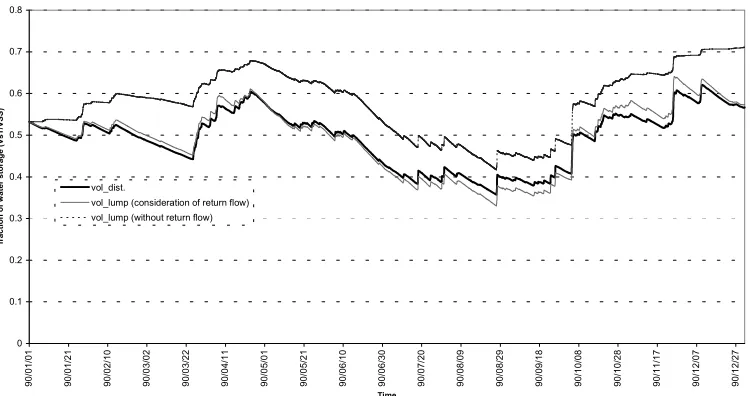
In this study, it was recognised that the phenomenon of return flow identified in the distributed model must also be considered in the lumped model. Figures 9 and 10 show the comparison of the simulation results obtained by the lumped TOPKAPI model with and without consideration of return flow. If the return flow was not considered in the lumped model, the dynamics of the soil water storage and the calculated discharges would be significantly different from those generated by the distributed model.

The Arno river basin case study

RIVER BASIN CHARACTERISTICS

The Arno river basin (Fig. 11a) drains an area of 8228 km2_, rising in the mountain Falterona (1654 m a.s.l) situated in the northern border of Casentino. The river flows in a south-west to north-east direction to the confluence with the Sieve river (836 km2_{) where it flows east to west to the river mouth.} Over its course, the Arno river is joined by major tributaries including the Greve river, Pesa stream, Elsa river and Era river on the left side, and the Bisenzio river and Omrone river on the right side. The watercourse of the river has a total length of approximately 245 km. Local climatic

0 200 400 600 800 1000 1200 1400 1600 1800 2000

90/11/21 90/11/22 90/11/23 90/11/24 90/11/25 90/11/26 90/11/27 90/11/28 90/11/29 90/11/30 90/12/01 90/12/02 90/12/03 90/12/04 90/12/05 90/12/06 90/12/07 90/12/08 90/12/09 90/12/10 90/12/11

Time

Discharge (m3/s)

Observed lumped (with return flow lumped no return flow

Di

sc

ha

rg

e (m

3s -1)

O b se rve d

L u m p e d w ith re tu rn flo w L u m p e d n o retu rn flo w

Fig. 9. Comparison of observed and modelled discharges for Casalecchio. Thick solid line: observed; dash line: lumped model with return flow; thin solid line: lumped model without consideration of return flow. Major flood events.

0 0.1 0.2 0.3 0.4 0.5 0.6 0.7 0.8

90/01/01 90/01/21 90/02/10 90/03/02 90/03/22 90/04/11 90/05/01 90/05/21 90/06/10 90/06/30 90/07/20 90/08/09 90/08/29 90/09/18 90/10/08 90/10/28 90/11/17 90/12/07 90/12/27

Time

fraction of water storage (VsT/VSS)

vol_dist.

vol_lump (consideration of return flow) vol_lump (without return flow)

F

Fiirreennzzee

S

S..GGiioovvaannnnii _{FFeerrrroovviiaa} F

Foorrnnaacciinnaa

P

Peessaa

S

Suubbbbiiaannoo

N

NaavveeddiiRRoossaannoo

Sieve

Casentino

Chiana

Valdarno Superiore

Elsa Era

Padule Fucecchio OmbronePistoiese

Bisenzio

Greve Pesa

L

Laatteerriinnaa

a) b)

c) d)

Fig. 11. Arno river basin: (a) river system, sub-basins and water level stations, (b) DEM map (legend: elevation above sea level in meter), (c) Soil type map, and (d) Land use map

tendencies produce the highest flooding risk in the period from September to January when winds from the south-west dominate.

Topography

The highest areas are found in the montains of Falterona and Pratomagno in the Casentino (Fig. 11b). The mean elevation of the whole river basin is 292 m a.s. l.. A DEM

data file with a grid scale of 200 m is available for the Arno river basin. In this study, the DEM is used with a grid size of 1km (see Fig. 11b).

Soils

Based on the SCS classification (Soil Conservation Service, 1972), a soil property map (see Fig. 11c and Table 4) is available giving hydrological soil types. For the whole

Table 4. Legend for pedological data (soil hydrological types)

No. Hydrological DESCRIPTION type of soil

(S.C.S/C.N.)

1 A With limited runoff potentiality. Contains deep sands with a very little lime and clay, and deep gravel of high permeability.

2 B With moderately low runoff potentiality. Contains the major part of the sandy soil that is less deep than the one in the group A, but the group as a whole has a high infiltration capacity even when saturated.

3 C With moderately high runoff potentiality. Contains thin soils having a considerable quantity of clay and colloidal material, while less than group D. The group has limited infiltration capacity when saturated.

basin, the major soil type is C, which comprises 57.9 % of the total area. This implies that more than half of the soils possess the hydrological characteristics of a thin soil layer with moderately-high runoff potential, containing a considerable quantity of clay and colloidal material, with limited infiltration capacity when saturated. Also, the soils are thin and of lower permeability in the mountain areas, while the soils in low-lying areas are thick and of moderately high permeability.

Vegetation and land use

The primary land uses in this catchment (see Table 5) are the classes of B (38.6%) and S (34.7%). In the mountain areas, most land use comprises shrub, undergrowth and overgrowth bush, while in the low-lying areas most land is suitable for arable farming.

di Rosano (Valdarno Superiore) and Firenze (Arno River) — are computed from hourly river levels by means of well-verified rating curves. The areal rainfall distribution was estimated using the Thiessen Polygon method.

Calibration of the TOPKAPI model

The model calibration was performed at a 1-hour time-step using the hydrological dataset of 1 July to 31 December 1992. The initial parameter values of the three basic components in the TOPKAPI model, the soil water, surface water and channel water components, were estimated from the literature (e.g. using the USDA parameter tables for the Green-Ampt infiltration model). The final parameter values were obtained by ‘trial and error’ on the basis of curve fitting.

Figures 12 to 16 show the comparison of the observed discharges and those computed at Firenze, Nave di Rosano, Fornacina, Subbiano and Ponte della Ferrovia, respectively, using the distributed TOPKAPI model. The model calibration performance statistics and the parameter values are listed in Table 6 and Table 7, respectively.

Validation of the TOPKAPI model

Using the parameter values of Table 7, simulations were carried out using the dataset for the period from 1 July to 31 December 2000. Comparison of observed and simulated hydrographs for the five stations is shown in Figs. 17 to 21. The model simulation performance statistics are shown in Table 8.

Discussion of results

Figures 12 to 21 demonstrate that the distributed TOPKAPI model (based on a DEM with a large grid size of 1000 m) performed well in simulating the floods in the Arno river basin. It did not simulate well the low flows mainly due to the absence of groundwater and lake/reservoir components in the present model. The oscillations at low flows shown in Figs. 12, 13, 17 and 18 for Firenze and Nave di Rosano reflect the effect of a reservoir located at Laterina (see Fig. 11).

Tables 6 and 8 show that the model performance in terms of the coefficient of determination (r2_{) in the validation}

period is lower than that in the calibration period, especially for Fornacina and Subbiano. This is very probably due to the poor quality of the measured water levels at the stations of Fornacina and Subbiano. For event 2 (11 July 2000) the measurements for Fornacina are significantly in error, because its peak is higher than the corresponding peaks at Table 5. Legend for land use data

No. Class Description

1 U Urban areas with continuous tissue

2 U1 Discontinuous urban areas

3 CA Forest and arboreal vegetation

4 B Vegetation of shrub, undergrowth and

overgrowth bush

5 C Herbaceous vegetation, meadow-pasture

6 CS Special cultivated areas, olive, vineyard

7 S Suitable for sowing

8 NV Areas without vegetation

9 P Humid areas

APPLICATION OF THE DISTRIBUTED TOPKAPI MODEL

Data availablity

Floods have been experienced in 1992, 1993 and 2000. It was decided to choose 1992 as a flood year for model calibration, and use the dataset for 2000 for model verification. Since most raingauges were concentrated in the Upper Firenze in 1992, it was decided to calibrate the TOPKAPI model only in the catchment to Firenze with an area of about 4325 km2_.

0 500 1000 1500 2000 2500

00/09/22 00/09/26 00/09/30 00/10/04 00/10/08 00/10/13 00/10/17 00/10/21 00/10/25 00/10/29 00/11/02 00/11/07 00/11/11 00/11/15 00/11/19 00/11/23 00/11/27 00/12/02 00/12/06 00/12/10 00/12/14 00/12/18 00/12/22 00/12/27 00/12/31

D a te

Discharge (m3/s)

Di

sc

h

ar

g

e (m

3s -1)

0 500 1000 1500 2000 2500

00/09/22 00/09/26 00/09/30 00/10/04 00/10/08 00/10/13 00/10/17 00/10/21 00/10/25 00/10/29 00/11/02 00/11/07 00/11/11 00/11/15 00/11/19 00/11/23 00/11/27 00/12/02 00/12/06 00/12/10 00/12/14 00/12/18 00/12/22 00/12/27 00/12/31

D a te

Discharge (m3/s)

Di

sc

h

ar

g

e (m

3s -1)

Fig. 12. Model calibration results compared with observed discharges at Firenze. Solid line: observed; Dash line: calculated. Major flood events.

0 100 200 300 400 500 600 700 800 900

00/09/22 00/09/26 00/09/30 00/10/04 00/10/08 00/10/13 00/10/17 00/10/21 00/10/25 00/10/29 00/11/02 00/11/07 00/11/11 00/11/15 00/11/19 00/11/23 00/11/27 00/12/02 00/12/06 00/12/10 00/12/14 00/12/18 00/12/22 00/12/27 00/12/31

Date

Discharge ( m3/sec)

Di

sc

ha

rg

e (

m

3s -1)

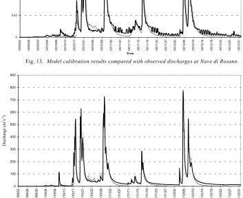
Fig. 13. Model calibration results compared with observed discharges at Nave di Rosano.

0 200 400 600 800 1000 1200 1400 1600

00/09/22 00/09/26 00/09/30 00/10/04 00/10/08 00/10/13 00/10/17 00/10/21 00/10/25 00/10/29 00/11/02 00/11/07 00/11/11 00/11/15 00/11/19 00/11/23 00/11/27 00/12/02 00/12/06 00/12/10 00/12/14 00/12/18 00/12/22 00/12/27 00/12/31

Date

Discharge ( m3/sec)

Dis

cha

rg

e (m

3s -1)

0 2 0 0 4 0 0 6 0 0 8 0 0 1 0 0 0 1 2 0 0 1 4 0 0

00/10/28 00/10/30 00/11/01 00/11/03 00/11/05 00/11/07 00/11/09 00/11/11 00/11/13 00/11/15 00/11/17 00/11/19 00/11/21 00/11/23 00/11/25 00/11/27 00/11/29 00/12/01 00/12/03 00/12/05 00/12/07 00/12/09 00/12/11 00/12/13 00/12/15 00/12/17 00/12/19 00/12/21 00/12/23 00/12/25 00/12/27 00/12/29 00/12/31

D a te

Discharge (m3/s)

Di

sc

h

ar

g

e (m

3s -1)

Fig. 15. Model calibration results compard with observed discharges at Subbiano.

Fig. 17. Model validation results compared with observed discharges at Firenze. Solid line: observed; Dash line: calculated. Major flood events.

0 50 100 150 200 250

00/09/22 00/09/26 00/09/30 00/10/04 00/10/08 00/10/13 00/10/17 00/10/21 00/10/25 00/10/29 00/11/02 00/11/07 00/11/11 00/11/15 00/11/19 00/11/23 00/11/27 00/12/02 00/12/06 00/12/10 00/12/14 00/12/18 00/12/22 00/12/27 00/12/31

Date

Discharge ( m3/sec)

Di

sc

h

ar

g

e (m

3s -1)

Fig. 18. Model validation results compared with observed discharges at Nave di Rosano.

Fig. 19. Model validation results compared with observed discharges at Fornacina.

0 2 0 0 4 0 0 6 0 0 8 0 0 1 0 0 0 1 2 0 0 1 4 0 0

00/10/28 00/10/30 00/11/01 00/11/03 00/11/05 00/11/07 00/11/09 00/11/11 00/11/13 00/11/15 00/11/17 00/11/19 00/11/21 00/11/23 00/11/25 00/11/27 00/11/29 00/12/01 00/12/03 00/12/05 00/12/07 00/12/09 00/12/11 00/12/13 00/12/15 00/12/17 00/12/19 00/12/21 00/12/23 00/12/25 00/12/27 00/12/29 00/12/31

D a te

Discharge (m£/s)

Di

sc

h

ar

g

e (m

3s -1)

Di

sc

h

ar

g

e (m

3s -1)

0 1 0 0 2 0 0 3 0 0 4 0 0 5 0 0 6 0 0 7 0 0

00/10/28 00/10/30 00/11/01 00/11/03 00/11/05 00/11/07 00/11/09 00/11/11 00/11/13 00/11/15 00/11/17 00/11/19 00/11/21 00/11/23 00/11/25 00/11/27 00/11/29 00/12/01 00/12/03 00/12/05 00/12/07 00/12/09 00/12/11 00/12/13 00/12/15 00/12/17 00/12/19 00/12/21 00/12/23 00/12/25 00/12/27 00/12/29 00/12/31

D ate

0 1 0 0 2 0 0 3 0 0 4 0 0 5 0 0 6 0 0 7 0 0 8 0 0 9 0 0

00/10/28 00/10/30 00/11/02 00/11/04 00/11/07 00/11/09 00/11/12 00/11/14 00/11/17 00/11/19 00/11/22 00/11/24 00/11/27 00/11/29 00/12/02 00/12/04 00/12/07 00/12/09 00/12/12 00/12/14 00/12/17 00/12/19 00/12/22 00/12/24 00/12/27 00/12/29

D a te

Discharge (m3/s)

Di

sc

h

ar

g

e (m

3s -1)

0 5 0 1 0 0 1 5 0 2 0 0 2 5 0 3 0 0

00/10/28 00/10/30 00/11/01 00/11/03 00/11/05 00/11/07 00/11/09 00/11/11 00/11/13 00/11/15 00/11/17 00/11/19 00/11/21 00/11/23 00/11/25 00/11/27 00/11/29 00/12/01 00/12/03 00/12/05 00/12/07 00/12/09 00/12/11 00/12/13 00/12/15 00/12/17 00/12/19 00/12/21 00/12/23 00/12/25 00/12/27 00/12/29 00/12/31

D a te

Discharge (m3/s)

Di

sc

h

ar

g

e (m

3s -1)

Fig. 21. Model validation results compared with observed discharges at Ponte di Ferrovia.

Table 6. TOPKAPI model calibration statistics in the Upper Firenze catchment in 1992

Station Fornacina Subbiano Ponte delle Nave di Firenze

Performance Ferrovia Rosano

statistics

R2 _{0.875 0.845 0.855 0.915 0.916}

r2 _{0.873 0.837 0.847 0.912 0.910}

r 0.934 0.915 0.920 0.955 0.954

Table 7. Calibration parameters for the different soil classes, land uses and channel orders

Soil ϑs−ϑr α ks L Land use

n

n

class (m s-1_{) (m) class (m}-1/3 _s-1_{) channel order (m}-1/3 _s-1₎

A 0.500 2.5 6.54E-04 1.20 U 0.060 I 0.045

B 0.535 2.5 6.06E-05 0.90 U1 0.100 II 0.040

C 0.425 2.5 1.89E-05 0.60 CA 0.200 III 0.035

D 0.417 2.5 1.67E-06 0.30 B 0.150 IV 0.030

C 0.100 V 0.025

CS 0.090

S 0.150

NV 0.100

P 0.010

Table 8. TOPKAPI model validation performance statistics for the Upper Firenze catchment in 2000

Station Fornacina Subbiano Ponte delle Nave di Firenze

Performance statistics Ferrovia Rosano

R2 _{0.739 0.626 0.820 0.891 0.878}

r2 _{0.732 0.608 0.811 0.889 0.858}