Spatial patterns in timing of the diurnal temperature cycle

www.hydrol-earth-syst-sci.net/17/3695/2013/ doi:10.5194/hess-17-3695-2013

© Author(s) 2013. CC Attribution 3.0 License.

Hydrology and

Earth System

Sciences

Spatial patterns in timing of the diurnal temperature cycle

T. R. H. Holmes1, W. T. Crow1, and C. Hain2

1_{USDA-ARS Hydrology and Remote Sensing Lab, Beltsville, MD, USA}

2_{Earth System Science Interdisciplinary Center, University of Maryland, College Park, Maryland, USA}

Correspondence to: T. R. H. Holmes ([email protected])

Received: 9 April 2013 – Published in Hydrol. Earth Syst. Sci. Discuss.: 15 May 2013 Revised: 13 August 2013 – Accepted: 21 August 2013 – Published: 1 October 2013

Abstract. This paper investigates the structural difference in

timing of the diurnal temperature cycle (DTC) over land re-sulting from choice of measuring device or model frame-work. It is shown that the timing can be reliably estimated from temporally sparse observations acquired from a constel-lation of low Earth-orbiting satellites given record lengths of at least three months. Based on a year of data, the spatial patterns of mean DTC timing are compared between temper-ature estimates from microwave Ka-band, geostationary ther-mal infrared (TIR), and numerical weather prediction model output from the Global Modeling and Assimilation Office (GMAO). It is found that the spatial patterns can be explained by vegetation effects, sensing depth differences and more speculatively the orientation of orographic relief features. In absolute terms, the GMAO model puts the peak of the DTC on average at 12:50 local solar time, 23 min before TIR with a peak temperature at 13:13 (both averaged over Africa and Europe). Since TIR is the shallowest observation of the land surface, this small difference represents a structural error that possibly affects the model’s ability to assimilate observations that are closely tied to the DTC. The equivalent average tim-ing for Ka-band is 13:44, which is influenced by the effect of increased sensing depth in desert areas. For non-desert areas, the Ka-band observations lag the TIR observations by only 15 min, which is in agreement with their respective theoret-ical sensing depth. The results of this comparison provide insights into the structural differences between temperature measurements and models, and can be used as a first step to account for these differences in a coherent way.

1 Introduction

In recent decades, Earth observation by satellite has pro-gressed from experimental to routine methods for monitor-ing many aspects of the hydrological cycle over land. For example, cloud water and precipitation from satellite sensors are now routinely ingested into numerical weather predic-tion (NWP) models (Bauer et al., 2011). Soil moisture ob-servations are at the point of entering into operational NWP assimilation schemes (Rosnay et al., 2011). Indirect obser-vations of the evaporative fluxes are now informing drought monitoring (Anderson et al., 2011; Hain et al., 2011). How-ever, one crucial parameter that is missing from this list is land surface temperature (LST). Even though it has been rou-tinely measured since the first Earth observation satellites, and physically based retrieval schemes for the above param-eters must account for LST in some way, it has yet to be successfully exploited as a stand-alone input to NWP mod-els. This is striking since LST is tightly linked (even more so than soil moisture) to land–atmosphere fluxes that are a pri-mary prediction goal for land models within NWP systems (Bosilovich et al., 2007).

models which utilize different soil layers and/or soil thermal capacities). This variability with depth together with a high spatial variability poses a challenge for the in situ valida-tion of LST, even though thermal infrared (TIR) measuring techniques can have high spatial resolutions (up to 1 km for global MODIS products for example). The resulting uncer-tainty regarding LST error characteristics is especially prob-lematic when time-varying structural errors go undetected. For remotely sensed LST estimates the bias may depend on emissivity, viewing angle, atmospheric opacity or sens-ing depth. In NWP models structural errors in LST may be introduced through the parameterization of the heat ca-pacity, layer depth or estimation of surface energy balance components. In previous attempts at assimilation of tem-perature observations into land surface models (Bosilovich et al., 2007; Reichle et al., 2010), time-varying bias was ad-dressed through rescaling of observations to match the auto-correlation and/or diurnal LST properties of models. While this may be the preferred strategy in a data assimilation ap-proach where the physics of the model has to be preserved, it squanders the opportunity to correct structural errors in the surface energy balance via comparison to satellite LST observations. This represents a missed opportunity because NWP centers are known to have diurnal biases in high-value predictions like precipitation (Dai and Trenberth, 2004).

In a comparison of temperature output from three different NWP models with in situ measurements, the depth difference between model and measurements could be resolved by con-sidering the timing, or phase, (φ) of the diurnal temperature cycle (DTC) (Holmes et al., 2012). It was shown that based on the annual average difference betweenφof measurements from different depths, the effect of 5 cm depth difference could accurately be corrected for. The logic behind this is that the difference in timing between two measurement or model systems represents the integrated effect of both depth difference and soil thermal properties. This timing difference is then assumed to be accompanied by an exponential change in amplitude according to heat flow principles (Van Wijk and de Vries, 1963).

Determiningφis relatively straightforward when the sam-pling frequency is much higher than the daily harmonic being sampled. This is true for NWP models, and also for obser-vations from geostationary satellites. However, for a single satellite in low Earth orbit the sampling frequency at any lo-cation is much lower: 1–2 observations per day (depending on the swath width). For such satellites we need to combine the observations from multiple platforms in order to reliably estimateφ. This was shown in Holmes et al. (2013), where vertical polarized Ka-band observations from four platforms were combined before determining the Ka-bandφ. That pa-per showed that Ka-band observations can be used to en-hance NWP temperature output, but only if the temperature series are properly reconciled in terms of timing, amplitude, and minimum of the diurnal temperature cycle. In the near future, the potential sampling of the DTC by Ka-band

sen-sors will be greatly enhanced by the constellation of satel-lites launched under the auspices of the Global Precipita-tion Measurement mission (Smith et al., 2007). In this pa-per we determineφ of NWP surface temperature estimates with an hourly output interval as provided by NASA’s Global Modeling and Assimilation Office (GMAO). We compare this to the φas determined from an inter-calibrated record of Ka-band brightness temperatures from five satellite plat-forms. As a third independent data source, we use thermal in-frared (TIR) LST retrievals from the geostationary Meteosat-9 satellite (centered at a longitude of 0◦), covering Europe and Africa.

When considered as group, these three sources (i.e., NWP-based, microwave-based and TIR-based) all provide inde-pendent information regarding LST and can theoretically be integrated together (via e.g. the assimilation of TIR and mi-crowave LST observations into the NWP model) or used to improve physical retrievals methods for ET and soil mois-ture which require ancillary LST information. However, be-fore these overarching goals can be accomplished, system-atic differences between these LST data sets – particularly as they relate toφ– must be understood. This will not only sup-port efforts to combine temperature from different sources, but may also help to better tailor a given temperature set to its function within physical retrieval models. For soil mois-ture remote sensing it may help to better adjust the temper-ature measurement to the sensing depth of the band that is actually used for the soil moisture retrieval. For precipita-tion, it may help efforts to improve the estimation of back-ground emissivity (Stephens and Kummerow, 2007). And finally, a proper reconciliation of thermal and microwave-based temperature may improve evaporation retrievals, such as the Atmosphere-Land Exchange Inverse model (ALEXI; Anderson et al., 1997), that currently depend on suboptimal gap-filling when clouds prevent TIR observations.

In preparation for a global merging of temperature data, this paper presents a global analysis of difference in DTC timing between Ka-band temperature estimates, TIR-based temperature estimates and NWP model output. The results of this comparison provide insights into diurnal differences between temperature measurements and models, and can be used as a first step to account for them in a coherent way.

2 Theory

Fig. 1. Simulation of effective temperature for Ka-band emission

for a dry (Teff(dry)) and a wet soilTeff(wet)). Assuming the

shal-low and deep layers are weighted equally inTeff(dry), the resulting

effective phase difference (dφ) is 54 min, about a fourth of the dif-ference (dφz) between the temperatures at their respective damping depths (z=zs).

For a surface temperature measurement, the average φ should be directly related to the incoming radiation, with a delay (damping) that is a function of the heat capacity of the soil or vegetation layer over the measurement depth of the sensor. When comparing two temperature measurements with the same spatial extent, the measurement depth will de-termine the level of damping of the diurnal temperature cycle (Van Wijk and de Vries, 1963) and the measurement with the earliest peak will represent the shallowest layer. TIR mea-surements have a sensing depth of about 50 µm, providing the shallowest practical measurement of LST. The timing of the maximum TIR temperature is typically reported between 60 and 90 min after solar noon (Choudhury et al., 1987; Betts and Ball, 1995; Fiebrich et al., 2003). Ka-band microwave emission has been shown to be a plausible alternative to TIR measurements, with much higher tolerance for clouds but a limited spatial resolution (Holmes et al., 2009). The sens-ing depth for Ka-band microwave emission, with a frequency of 37 GHz, is slightly deeper than TIR and varies with soil moisture. For most land surfaces it is assumed to be around 1 mm. Accordingly, theφderived from Ka-band emission is expected to be slightly behind that observed using TIR. Only in very dry areas with no vegetation is the Ka-band sensing depth potentially much deeper, on the order of cm’s (Ulaby et al., 1986), and theφof Ka-band can be further delayed. To illustrate the difference Fig. 1 simulates the effect of sensing depth on Ka-bandφfor a wet and a dry soil. The damping of the temperature harmonic with a period of a day can be described by a phase shift (dφ) proportional to the vertical distance (dz) divided by the damping depth (zD). The damp-ing depth is defined as the dzover which the amplitude of the harmonic is reduced by 63 %, and is an expression of the

thermal properties of the soil:

zD=

s

2a

2πf, (1)

whereais the thermal diffusivity (m2s−1) andf is the fre-quency (s−1) of the harmonic. For a dry soil (a=0.15e−6) Eq. (1) yields an estimate ofzD=6.5 cm. Estimates of the temperature sensing depth (zS) of 1 mm for a wet soil to 1 cm for a dry soil are given in Ulaby et al. (1986). The difference inzS for microwave Ka-band emission between a dry sandy soil and a wet soil is therefore about 9 mm. Dividing this by the dry soilzDof 6.5 cm equates to a 3 h 36 min shift inφ be-tween the soil layers at the lower ends of these sensing depths (dφz). Because the shallower soil depths weigh more heav-ily in the measured emission, and they have larger diurnal amplitudes, they affect the timing of the DTC more strongly. Therefore, the shift in phase (dφ) of actual measured Ka-band emission, originating from the entire soil profile, is es-timated as dφz/4, or 54 min (see Fig. 1). Observational evi-dence of this dφwill be discussed in Sect. 5.

3 Materials

In this study we compare three independent land tempera-ture measurements, two from satellite measurements and one based on a global NWP model. The satellite observations in-clude a number of Ka-band sensors with global coverage and TIR measurements from a geostationary satellite. All sets are available for the full year 2009 and are described below.

3.1 Satellite Ka-band brightness temperature

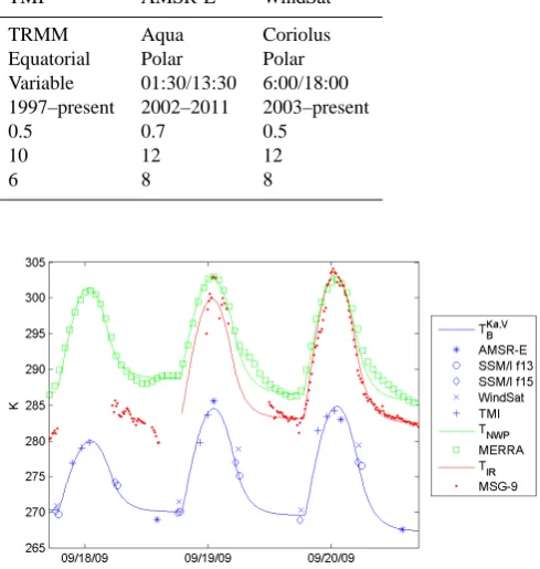
Table 1. Specifications of satellite sensors providing Ka-band microwave observations used for land surface temperature estimation.

Sensor SSM/I TMI AMSR-E WindSat

Satellite DMSP F13, F15 TRMM Aqua Coriolus Orbit Polar Equatorial Polar Polar Equatorial overpass 6:00–22:00 Variable 01:30/13:30 6:00/18:00 Operational 1987–present 1997–present 2002–2011 2003–present

Accuracy (K) 0.4 0.5 0.7 0.5

Spatial resolution (km) 33 10 12 12 Over-sampling in 0.25◦grid 1 6 8 8

satellites, allowing for an inter-calibration of the satellites as described in Holmes et al. (2013).

Within the microwave spectrum,T_BKa, Vis the most appro-priate frequency to retrieve LST as it balances a reduced sen-sitivity to soil surface characteristics with a relatively high atmospheric transmissivity (Colwell et al., 1983). In Holmes et al. (2009) it was further shown that an assumption of a con-stant land surface emissivity can be used to obtain LST esti-mates from Ka-band with relatively high sensitivity, if not ab-solute accuracy. For the purpose of this paper no conversion to physical temperature is needed since only the timing of the DTC is analyzed here, not its amplitude. This means that for this paper the assumption of constant emissivity needs only to hold over the course of the day, because there is no effect of absolute bias in LST on the analysis. Still, the lin-ear relationship between Ka-band and LST does potentially break down under frozen soil conditions or during precipita-tion events. This leads to the formulaprecipita-tion of two condiprecipita-tions for the Ka-band data. To avoid frost conditionsT_BKa, Vmust be above 260 K, a rough estimate of the Ka-band freezing point determined in Holmes et al. (2009). The spatial stan-dard deviation of all Ka-band observations within a 0.25 de-gree grid box is used as an indicator for measurement uncer-tainty; above-normalσKa, Vis attributed to active precipita-tion (Holmes et al., 2013). The second condiprecipita-tion is therefore based on σKa, V; a gridbox average is rejected if σKa, V is more than 1 K above the annual mean for that grid box. The Ka-band temperature set is referred to in the following as TKa. An example of the resulting sampling of the combined TKa is given in Fig. 2 for three days in September 2009. In the same graph the NWP and infrared resource are shown; they are described below.

3.2 NWP surface temperature

The modeled temperature data set was acquired from NASA’s GMAO and their Modern Era Retrospective-analysis for Research and Applications (MERRA) (http:// gmao.gsfc.nasa.gov/research/merra, Rienecker et al., 2011). MERRA products are generated using Version 5.2.0 of the GEOS-5 DAS (Goddard Earth Observing System (GEOS) Data Assimilation System (DAS)) with the analysis and model output both at a spatial resolution of 0.5◦latitude by

Fig. 2. Three days of diurnal cycles of TKa, TNWP, and TIR in

September 2009. All variables are explained in Sect. 3. Solid lines represent the fitted DTC, as described in Sect. 4.

0.67◦ _{longitude, and with a 6-hourly analysis cycle.} Two-dimensional diagnostics describing the radiative and physical state of the surface are available as hourly averages.

Surface processes in MERRA are based on the NASA Catchment land surface model (Ducharne et al., 2000; Koster et al., 2000). Each MERRA grid cell contains several irreg-ularly shaped tiles, and each tile is further divided into sub-tiles based on their modeled hydrological state: saturated, un-saturated, and wilting. The surface temperature of a grid cell is obtained by area-weighted averaging of the surface tem-peratures of all sub-tiles within the grid cell. The sub-tile sur-face temperatures are prognostic variables of the model and represent a bulk surface layer with a small but finite heat ca-pacity. For all vegetation classes except broadleaf evergreen trees, this bulk surface layer represents the vegetation canopy and a surface layer at the top of the soil column (effective layer depth<1 mm).

Fig. 3. Main characteristics of the diurnal temperature cycle and the

definition of the phase of the DTC (φ).

3.3 Geostationary thermal-infrared-based LST

TIR-based LST (TIR) is an operational product of the Land Surface Analysis–Satellite Applications Facility (LSA-SAF, see http://landsaf.meteo.pt). It is generated using the split-window channels (10.8 and 12.0 µm) of the Spinning En-hanced Visible and InfraRed Imager (SEVIRI) on board the geostationary Meteosat second-generation (MSG) satellite; therefore a high temporal resolution (15 min) of the data is possible (Kabsch et al., 2008; Trigo et al., 2011).

These LST data are provided on a 3 km equal-area grid. When regridding onto a 0.25◦ regular grid, this results in a large over sampling of the grid box. If more than two-thirds of the 3 km observations are masked out for a par-ticular location and time, then that sampling average is re-jected. This threshold increases the amount of data discarded by the cloud filter forTIR. We further limit the coverage of the METEOSAT-9 to the domain covered with an Earth inci-dence angle up to 78◦_{, avoiding artifacts at large view angles.} The resulting METEOSAT-9 domain covers Africa, Europe and the Middle East. In Fig. 2 the high sampling rate ofTIR is apparent, as are gaps (attributed to clouds) on day 1 and 2 of this example series.

4 Methods

In Holmes et al. (2012) it was shown that a relative estimate ofφcan be determined by fitting a simple harmonic model to a temperature time series. This worked well enough when only φ differences between temperature sets are needed. However, the values itself are hard to interpret since the ac-tual shape of the DTC rarely resembles a perfect harmonic shape, resulting in differences between the time of maximum temperature and the peak of the harmonic.

In this paper we adapt a more sophisticated model of the DTC as described by Göttsche and Olesen (2001). This harmonic-exponential DTC model improves the fit along the

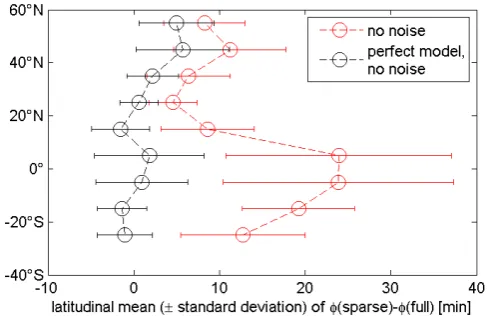
Fig. 4. Effect of sparse temporal sampling (at TKa observation

times) on retrieval ofφ.

cooling limb of the DTC and allows for better leveraging of observations at all times. In addition, it yields an estimate of φ that can be more readily interpreted as the time lag be-tween solar noon and peak temperature. The DTC model by Göttsche and Olesen (2001) was originally intended as a five-parameter model, but a subsequent addition to param-eterize total (atmospheric) optical depth increased this to six (Göttsche and Olesen, 2009). A recent comparison paper (Duan et al., 2012) discussed several variants of the DTC model by Göttsche and Olesen (2001) and showed that im-provements were caused by adding an additional free param-eter related to the day length. In this paper we have to reduce the number of free parameters to limit the computational de-mands and speed conversion to a solution. Therefore we sim-plify the five-parameter model (Göttsche and Olesen, 2001) to have only three free parameters. A comparison study (not shown) demonstrated that this does not reduce the accuracy of the meanφ as determined over longer time series. The method is detailed below.

In Göttsche and Olesen (2001) the DTC model (Tpar) is pa-rameterized as a function of the time of maximum (tm), day length (ω), diurnal amplitude (Ta), diurnal minimum (T0), change in minimum from day to day (δT), and start of the attenuation function (ts):

Tpar(t )=T0+Tacos

π

ω(t−tm)

, t < ts (2) Tpar(t )=T0+δT+

h

Tacos

π

ω(ts−tm)

−δTie −(t−ts)

k _{, t}≥ts.

Figure 3 shows an example ofTparand illustrates the defini-tions of its parameters. The attenuation constantkis calcu-lated by making the first derivatives of the day- and nighttime equation equal at timets:

k=ω π

"

1 tan π_ω(ts−tm)

− δT

Tasin π_ω(ts−tm)

#

To limit the degrees of freedom and increase conversion to a solution, in this studytsis fixed so that half of the decrease in temperature (over the cooling-down limb) is described by the exponential equation. That way,tscan be calculated from tmandωas

ts=tm+ ω πarccos

₁

2

1+δT Ta

. (4)

For a given day and temperature set, first-guess estimates ofT0andTaare determined based on the minimum and max-imum recorded observations within the 24 h period from sun-rise to sunsun-rise. Similarly,δT is initialized based on the dif-ference betweenT0of the current and the next day, if avail-able. Solar noon (tn) andωare calculated based on latitude and day of year according to general solar position calcula-tions (Cornwall et al., 2003). Defining φ as the offset be-tween optimized time of maximum temperature and solar noontm=tn+φ, there are three free parameters:φ,T0, and Ta. Of these, onlyT0andTavary from day to day;φis as-sumed constant over the data range. With these assumptions it is possible to determineφin an iterative optimization loop that minimizes the squared errors (E) betweenTparand the data series. In Fig. 2 examples ofTparare shown, as fitted for the three LST resources used in this manuscript.

The above-described fitting of the DTC model is possible for days where the available samples are sufficient to con-strain the estimates ofT0 andTa, together with at least two further samples to anchorφ. The optimization loop is there-for only applied to days where the number of samples (N (d)) is four or more. Furthermore, in order to assure a reasonable fit with the clear-sky DTC model, we limit the analysis to days where the temperature does not dip below freezing, and where the maximum temperature is close to the meantm. Fi-nally, in order to have an acceptable signal-to-noise ratio we focus on days where the estimated amplitude exceeds 5 K. In summary, only days (d) where the following conditions are met are included in the optimization loop to determine the timing for each temperature set:

1. N (d) >=4,

2. T0(d)above freezing point, 3. tm(d)within 2 h of meantm, and 4. Ta>5 K.

The exact thresholds applied in these four conditions are cho-sen to select the most optimal days for the analysis, without overly limiting the number of usable data days in a given time period. Still, the effect of these criteria on the number of usable days results in the need for a time period of a year to generate sufficient data days to compensate for the uncer-tainty in the satellite observations, particularly in the tropical and boreal zones with limited diurnal amplitude. The above considerations and conditions also point out the need for five

different satellites to estimate the timing ofTKa. The AMSR-E satellite is crucial to satisfy condition (3) because its ob-servation falls close to the maximum of the diurnal at 13:30. The WindSat and SSM/I satellites help constrain the early morning minimum and the afternoon cooling limb. The TMI observations increase the number of data days by helping to satisfy conditions (1) and (3), and are indispensable for the inter-calibration of the sensors.

To test if the sampling ofTKa results in a bias relative to the hourly sampling of MERRA, we looked at the change in apparent timing forTNWP, when only observations at the overpass times of the Ka-band set are used. The effect of sparse sampling on theφis averaged by latitude and shown in Fig. 4. By using MERRA model output for this sensitivity analysis we cannot test for the effect of noise in the observed data. Moreover, the diurnal harmonic ofTNWP may have a different bias relative to the DTC model thanTKa. This po-tential mismatch in DTC shape may be responsible for the bias as shown around the Equator for the first test with no noise and imperfect model. We repeat the test after removing the mismatch in the DTC model, resulting in a perfect model with no noise. Only if this assumption is valid do we expect to have no bias. These results indicate that the uncertainty as introduced by the limited sampling frequency of the Ka-band data is small enough to measure Ka-band timing from this set of sensors, but only if the DTC model accurately represents the measuredTKa.

5 Results

The above-described method to determineφis applied to the three temperature recordsTKa,TNWP, andTIR (described in Sect. 3) for the data year 2009. The resulting (0.25◦) maps of φare displayed in Fig. 5 for Europe and Africa, the spatial domain of MSG-9.

On average theTKapeaks at 13:44 with lower values over Europe and highest values over deserts and tropical rain-forests. Later values of peak temperature in deserts can be explained by the deeper sensing depth of Ka-band emission under dry soil conditions (see Sect. 2). In fact, the areas with latestφ correspond closely to sand deserts; see for exam-ple the Arabian Peninsula in Fig. 5a where the Rub’al Khali Erg shows up causing an hour delay of the Ka-bandφ. This feature was earlier noted in terms of day/night difference of SSM/I channels (Prigent et al., 1999), polarization difference of AMSR-E channels (Jiménez et al., 2010), and even more comparable to the present analysis, in terms of phase dif-ference between microwave and TIR temperature (Norouzi et al., 2012). In this later study the third component derived from a principal component analysis (PCA) was attributed to the phase of the diurnal cycle. The close resemblance of the spatial features generally supports this conclusion.

Fig. 5. 2009 meanφforTKa(a),TNWP(b), andTIR(c). (d) North–south transect of meanφ.

Fig. 6. 2009 meanφ determined forTKa, TIR, andTNWP within selected IGBP land cover types. BetweenTNWP andTIRthere is

a fairly constant dφof 20 min.TKaagrees withTIRover land surface types with little or no barren surface.

variation. Another unexpected feature in the maps ofφ (TKa) is the earlier phase over mountainous areas (e.g., the Rif mountains in NW Africa, the Caucasus). Both features will be discussed in relation to theφofTIRandTNWP.

ForTNWP, with a mean peak temperature at 12:50, there is much less spatial variation inφwith the notable exception of tropical rainforest; see Fig. 5b. The distinctly different results over rainforest with values around 13:30 are explained by a higher heat capacity as parameterized for areas classified as tropical forest in the MERRA model. At more northern latitudes, higherφvalues are also found over the forest areas of the eastern European plain. Areas with lowestφseem to correspond with high-elevation areas.

Fig. 7. Timing difference [h]: (a)φ (TNWP)−φ (TIR), average dφ= −23 min; and (b)φ (TKa)−φ (TIR), average dφ=30 min. The color bar

is centered on the average for each map.

expansive and includes more generally the humid tropical zone of Africa.

Figure 5d shows a north–south transect of theφas deter-mined forTKa,TNWP, andTIR – all averaged over the lon-gitude extent of 0–30◦E. All sets have a delayedφ around the Equator, which forTNWPis explained by the higher heat capacity as parameterized for tropical rainforest. ForTKaand TIR, with little to no penetration of the canopy layer, the de-lay inφmight more plausibly have to do with the effect of a diurnal pattern in cloudiness which can cause a delay in the peak solar radiation. If this is true, then MERRA predicts a correct delay in timing but for the wrong reason. Superim-posed on this tropical signature,TKaclearly shows a delayed φover (seasonally) dry areas in northern and southern Africa, explained by the deeper sensing depth.

The patterns inφand differences between the sets seem to align with particular land surface types. Therefore, MODIS land cover maps (MCD12C1, Version 051) are used to study φby land surface type (International Geosphere-Biosphere Programme (IGBP) classification). Figure 6 lists the aver-age values as obtained over selected surface types between longitudes 0 to 30◦E. This indeed confirms the general re-lation with vegetation type – all sets exhibit delayedφover broadleaf forest compared to the cropland and Europe selec-tions. Only forTKaare delays inφrecorded over the savan-nah and desert land cover types.

As a consequence of the general agreement in φ be-tweenTNWP andTIR, the spatial map of their difference in φ is remarkably homogenous:φ (TIR)−φ (TNWP)=27 min (±15 min) for 79 % of the land area (see Fig. 7a). Areas with larger differences are found at the edge of land masses and mountain ranges, whereφ (TIR) can be up to 1.5 h behind φ (TNWP)as shown in Fig. 7. Interestingly, these areas also show up in Fig. 7b, sometimes even indicating thatTKapeaks earlier thanTIR, which is not physically realistic. Because of this, we look toTIR for the explanation of these anoma-lies. Insofar as these features line up with mountain ranges, they are tentatively attributed to azimuth angle effects onTIR. Since they are retrieved from a geostationary satellite (MSG-9) located at the prime meridian, variations in azimuth angle might explain the earlierφover mountains to the northwest of the satellite and the delayedφover ranges that are to the east of the satellite. Such azimuth angle effects are muted within TKa as this is composed of observations with vary-ing azimuth angles (and obviously play no role in the NWP record). Along the coast in the tropical zone large negative anomalies show up inTIRrelative toTKaandTNWPthat can-not be explained by mountains. In these areas there are few days without clouds, and we therefore attribute this to a fail-ure of the cloud mask inTIR.

The timing difference betweenTKaandTIRis greatest over the driest parts of Africa, whereTKais 57 min (±25 min) be-hindTIR inφ; see Fig. 7b. This average dφagrees with the theoretical calculations of Sect. 4. This suggests that the large increase inφKaover dry areas can be quantitatively explained

by an increase in temperature sensing depth. As expected for all but the driest soils (especially when covered with vege-tation) the difference is much closer to zero over the rest of Africa and Europe. For example, over Europe the φ maps show thatTKais only 14 min (±12 min) behindTIR.

In order to test if the discussed patterns inφ are stable throughout the year, the procedure to calculate φ was re-peated for 3-month seasonal periods. The seasonal results confirmed the large-scale north–south patterns as shown in Fig. 5d, giving confidence that land cover type is the main de-terminant forφ, rather than seasonal varying factors like soil wetness or cloudiness. Furthermore, it suggests thatφ may be considered relatively constant in time; the spatial standard deviation of the seasonal anomaly from the annualφis 6 min forTNWP, 7 min forTIR, and 14 min forTKa.

6 Global results

This section will briefly discuss the spatial patterns in tim-ing on the global scale, as calculated forTKaandTNWP. The geostationary TIR resource is not yet available as a consoli-dated global data set and is therefore not included here. The global maps ofφ confirm the land cover features as found over Africa and Europe and discussed in Sect. 5. In the global φmap ofTKa(see Fig. 8, top), delays of up to an hour from the meanφof 13:37 for desert areas are matched with similar delays in the deserts of Australia and central Asia. Similarly, the apparent delay in timing over tropical forest is repeated over the Amazon.

ForTNWP (Fig. 8, middle panel), φis generally between 12:30 and 13:00 with three main exceptions. Tropical forest show up with highly delineated delays inφof up to 40 min over the Amazon and Indonesia, in close agreement with the above discussed Congo Basin in Africa. As discussed earlier, this is explained by the increased heat capacity of the surface layer as parameterized for tropical forest by MERRA. Be-cause this is a static feature of MERRA, the resulting spatial pattern ofφis expected to remain stable from year to year, as long as the same land classification is used.

Another feature that shows up is earlier φ over moun-tainous and high-elevation areas. Although this feature was discussed earlier, it is much more pronounced over the An-des and Himalaya. Since it appears in bothTKa andTNWP, it most likely reflects an actual pattern in diurnal heat ex-change. Possible physical mechanisms for this include the effect of cooler air temperatures at higher elevation on sensi-ble heat flux, diurnal patterns in orographic cloud formation, and slope effects on incoming solar radiation as described in Senkova et al. (2007).

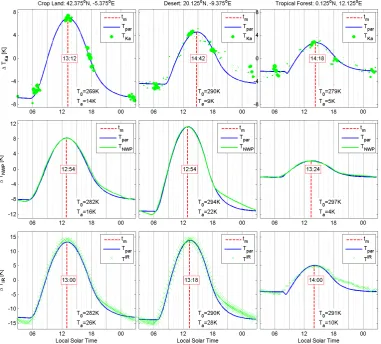
Fig. 9. Example of overall fitTparto the three LST estimates for selected locations. The displayed data reflect the annual average deviation

1T=T−(T0+Ta/2)for each hour of day.

freezing and a diurnal amplitude of 5 K or higher, theφ cal-culated in these northern regions (with weak diurnal radia-tive forcing) is based on a relaradia-tively limited amount of long cool days. Unfortunately, TIR observations are not available at those high latitudes to positively attribute this anomaly to TNWP.

On average TKa peaks 40 min later than TNWP (Fig. 8, lower pane). In the temperate climates and the tropics the dφis close to this average. Bigger differences appear in the desert areas where Ka-band peaks up to 2 h afterTNWP, cor-responding to a deeper sensing depth. The boreal areas show smaller differences resulting from the delayedφofTNWPas discussed above. Due to the close link with land cover and geological features it is expected that these patterns of dφ will remain relatively stable from year to year.

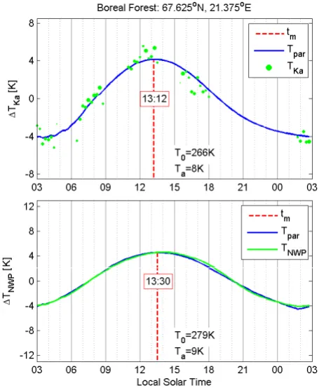
Each of these features deserves discussion in more detailed studies where ground measurements are available for com-parison. Such regional studies would benefit from relaxing some of the parameters that were fixed in this global study, allowing for improved fit of the DTC model (Tpar) over par-ticular biomes. In support of the main features that were

dis-cussed in this paper, we conclude with two graphs that sum-marize the overall fit ofTparto the three LST estimates over four key biomes; see Figs. 9 and 10. The displayed data re-flect the annual average by hour of day for a single grid cell. Observational data are corrected for the effect of sparse sam-pling on the average. These graphs show that even though the fit ofTparis not perfect at all times of day, it does not appear to impact the relative conclusions of the study. All sets have a clear delay inφ over tropical forest that is picked up by the fittedTparin the presented examples. In contrast, the late φofTKa stands out from the other sets in the desert exam-ple. In boreal forestTNWPhas a relative delay inφthat is not reflected inTKa.

7 Conclusions

T. R. H. Holmes et al.: Timing of the diurnal temperature cycle 3705

the annual average deviation

∆T

=

T

−

(T

+

T

/2)

for each hour of day.

Fig. 10.

Example of overall fit of

T

to LST estimate in the boreal region. The displayed data reflects the

annual average deviation

∆T

=

T

−

(T

+

T

/2)

for each hour of day.

23

Fig. 10. Example of overall fit ofTparto LST estimate in the bo-real region. The displayed data reflect the annual average deviation

1T=T−(T0+Ta/2)for each hour of day.

radiometers. The spatial patterns inφ for each temperature set are explainable based on consideration of land surface type and basic physics describing the penetration depth of microwave observations. An interesting observation is that over tropical forest the timing is delayed by 30 to 40 min rel-ative to the average phase in both satellite data sets. While this delay is accurately modeled in MERRA, it may be for the wrong reason if the delay is caused by a diurnal variabil-ity of cloudiness rather than an increase in heat capacvariabil-ity of the sampled surface layer. On the other hand, deserts cause a delay in the timing of Ka-band diurnal temperature cycle which is not matched in the TIR nor MERRA estimates. This is explained by a deeper sensing depth for the microwave ob-servations in dry soils and becomes especially extreme in dry sand deserts.

The timing of Ka-band observations outside of the desert and semi-desert areas is (on average) 15 min after TIR. This small delay of the DTC compared to TIR agrees with a slightly deeper sensing depth for Ka-band, 50 µm vs. 1 mm. On the other hand, MERRA seems to model the average peak of the DTC about 23 min before that of TIR, which should be the shallowest observation possible of the land surface. Therefore, if the goal is to model the surface temperature, it appears the heat capacity of the surface layer is set slightly too low in MERRA. To put this timing difference in con-text of biases in T, there are two main considerations. First,

if this timing difference is indeed a result of a low bias in heat capacity, then the associated overestimation of the diur-nal amplitude would be 10 % for a 23 min timing difference (Holmes et al., 2012). Secondly, the timing difference will in-troduce a diurnal bias term. These two effects together result in a harmonic diurnal bias with an amplitude that depends on the diurnal temperature range (for example, 1.4 K bias for aT with 20 K diurnal range). This type of time-variant structural bias terms are much harder to account for in data assimilation approaches than constant bias terms.

This study has identified structural differences in diurnal timing between MERRA, TIR and Ka-band-based land sur-face temperature estimates and constitutes one of the first global analyses of the effects of vegetation and sensing depth on the timing of different temperature measurements. Even though the global maps of the timing for each set are based on the year 2009, these features are expected to be relatively stable from year to year. The presented analysis of the timing of the diurnal temperature cycle offers a means to account for time-variant bias terms between temperature records in a physically consistent way. With these maps we can now reconcile temperature records in terms of their diurnal tim-ing, opening the way for studies that look at differences in diurnal amplitude and daily minimum, and ultimately for a global merger of temperature data sets.

Acknowledgements. This work was funded by NASA

through the research grant “The Science of Terra and Aqua” (NNH09ZDA001N-TERRAQUA). The authors would like to thank the Global Modeling and Assimilation Office (GMAO) and the GES DISC (both at NASA Goddard Space Flight Center) for the dissemination of MERRA. USDA is an equal opportunity provider and employer.

Edited by: W. Wagner

References

Anderson, M. C., Norman, J. M., Diak, G. R., Kustas, W. P., and Mecikalski, J. R.: A two-source time-integrated model for esti-mating surface fluxes using thermal infrared remote sensing, Re-mote Sens. Environ., 60, 195–216, 1997.

Anderson, M. C., Hain, C., Wardlow, B., Pimstein, A., Mecikalski, J. R., and Kustas, W. P.: Evaluation of drought in-dices based on thermal remote sensing of evapotranspiration over the continental United States, J. Climate, 24, 2025–2044, doi:10.1175/2010jcli3812.1, 2011.

Bauer, P., Auligné, T., Bell, W., Geer, A., Guidard, V., Heilliette, S., Kazumori, M., Kim, M. J., Liu, E. H. C., and McNally, A. P.: Satellite cloud and precipitation assimilation at operational NWP centres, Q. J. Roy. Meteor. Soc., 137, 1934–1951, 2011. Betts, A. K. and Ball, J. H.: The FIFE surface diurnal cycle climate,

J. Geophys. Res.-Atmos., 100, 25679–25693, 1995.

a coupled land-atmosphere data assimilation system, J. Meteo-rol. Soc. Jpn., 85, 205–228, 2007.

Choudhury, B. J., Idso, S. B., and Reginato, R. J.: Analysis of an empirical model for soil heat flux under a growing wheat crop for estimating evaporation by an infrared-temperature based energy balance equation, Agr. Forest Meteorol., 39, 283–297, 1987. Colwell, R. N., Simonett, D. S., and Ulaby, F. T. (Eds.): Manual

of remote sensing, in: Interpretation and Applications, 2nd Edn., Vol. II, Falls Church, 1983.

Cornwall, C., Horiuchi, A., and Lehman, C.: General solar po-sition calculations, available at: http://www.esrl.noaa.gov/gmd/ grad/solcalc/solareqns.PDF (last access: May 2013), 2003. Dai, A. and Trenberth, K. E.: The diurnal cycle and its depiction in

the Community Climate System Model, J. Climate, 17, 930–951, doi:10.1175/1520-0442(2004)017<0930:TDCAID>2.0.CO;2, 2004.

Duan, S.-B., Li, Z.-L., Wang, N., Wu, H., and Tang, B.-H.: Evalu-ation of six land-surface diurnal temperature cycle models using clear-sky in situ and satellite data, Remote Sens. Environ., 124, 15–25, 2012.

Ducharne, A., Koster, R., Suarez, M., Stieglitz, M., and Praveen, K.: A catchement-based approach to modeling land-surface pro-cesses in a GCM – 2. Parameter estimation and model demon-stration, J. Geophys. Res., 105, 24809–24822, 2000.

Fiebrich, C. A., Martinez, J. E., Brotzge, J. A., and Basara, J. B.: The Oklahoma Mesonet’s Skin Temperature Network, J. Atmos. Ocean. Tech., 20, 1496–1504, doi:10.1175/1520-0426(2003)020<1496:TOMSTN>2.0.CO;2, 2003.

Göttsche, F.-M. and Olesen, F. S.: Modelling of diurnal cycles of brightness temperature extracted from METEOSAT data, Re-mote Sens. Environ., 76, 337–348, 2001.

Göttsche, F.-M. and Olesen, F.-S.: Modelling the effect of optical thickness on diurnal cycles of land surface temperature, Remote Sens. Environ., 113, 2306–2316, 2009.

Hain, C. R., Anderson, M. C., Zhan, X., Svoboda, M., Wardlow, B., Mo, K., Meckalski, J. R., Kustas, W. P., and Brown, J.: A GOES Thermal-Based Drought Early Warning Index for NIDIS, in: NOAA’s National Weather Service, Science and Techn. Inf. Cli-mat. B., Fort Worth, TX, 2011.

Holmes, T. R. H., De Jeu, R. A. M., Owe, M., and Dol-man, A. J.: Land surface temperature from Ka band (37 GHz) passive microwave observations, J. Geophys. Res., 114, D04113, doi:10.1029/2008JD010257, 2009.

Holmes, T. R. H., Jackson, T. J., Reichle, R. H., and Basara, J. B.: An assessment of surface soil temperature products from numerical weather prediction models using ground-based measurements, Water Resour. Res., 48, W02531, doi:10.1029/2011WR010538, 2012.

Holmes, T. R. H., Crow, W. T., Yilmaz, M. T., Jackson, T. J., and Basara, J. B.: Enhancing model-based land surface temperature estimates using multiplatform microwave observations, J. Geo-phys. Res.-Atmos., 118, 1–15, 2013.

Jiménez, C., Catherinot, J., Prigent, C., and Roger, J.: Relations between geological characteristics and satellite-derived infrared and microwave emissivities over deserts in northern Africa and the Arabian Peninsula, J. Geophys. Res., 115, D20311, doi:10.1029/2010JD013959, 2010.

Kabsch, E., Olesen, F. S., and Prata, F.: Initial results of the land surface temperature (LST) validation with the Evora, Portugal

ground-truth station measurements, Int. J. Remote Sens., 29, 5329–5345, doi:10.1080/01431160802036326, 2008.

Koster, R., Suarez, M., Ducharne, A., Stieglitz, M., and Praveen, K.: A catchement-based approach to modeling land-surface pro-cesses in a GCM – 1. Model structure, J. Geophys. Res., 105, 24809–24822, 2000.

Norouzi, H., Tenimi, M., AghaKouchak, A., Azarderakhsh, M., and Khanbilvardi, R.: On the effect of land cover type on the diurnal cycle of microwave brightness tmperatures, IEEE Geosci. Re-mote Sense., submitted, 2012.

Parinussa, R. M., Holmes, T. R. H., and De Jeu, R. A. M.: Soil moisture retrievals from the WindSat spaceborne polarimetric microwave radiometer, IEEE Trans. Geosci. Remote, 50, 2683– 2694, doi:10.1109/TGRS.2011.2174643, 2012.

Prigent, C., Rossow, W. B., Matthews, E., and Marticorena, B.: Microwave radiometric signatures of different surface types in deserts, J. Geophys. Res., 104, 12147–12158, doi:10.1029/1999JD900153, 1999.

Reichle, R. H., Kumar, S. V., Mahanama, S. P. P., Koster, R. D., and Liu, Q.: Assimilation of satellite-derived skin temperature ob-servations into land surface models, J. Hydrol., 11, 1103–1122, doi:10.1175/2010JHM1262.1, 2010.

Rienecker, M. M., Suarez, M. J., Gelaro, R., Todling, R., Bacmeis-ter, J., Liu, E., Bosilovich, M. G., Schubert, S. D., Takacs, L., Kim, G.-K., Bloom, S., Chen, J., Collins, D., Conaty, A., da Silva, A., Gu, W., Joiner, J., Koster, R. D., Lucchesi, R., Molod, A., Owens, T., Pawson, S., Pegion, P., Redder, C. R., Re-ichle, R., Robertson, F. R., Ruddick, A. G., Sienkiewicz, M., and Woollen, J.: MERRA: NASA’s Modern-Era Retrospective Anal-ysis for Research and Applications, J. Climate, 24, 3624–3648, doi:10.1175/JCLI-D-11-00015.1, 2011.

Rosnay, P. D., Drusch, M., Balsamo, G., Albergel, C., and Isak-sen, L.: Extended Kalman Filter soil-moisture analysis in the IFS, ECMWF Newsletter, pp. 12–15, available at: http://www.ecmwf. int/publications/newsletters/pdf/127.pdf (last access: May 2013), 2011.

Senkova, A. V., Rontu, L., and Savijarvi, H.: Parametrization of oro-graphic effects on surface radiation in HIRLAM, Tellus A, 59, 279–291, doi:10.1111/j.1600-0870.2007.00235.x, 2007. Smith, E., Asrar, G., Furuhama, Y., Ginati, A., Mugnai, A.,

Naka-mura, K., Adler, R., Chou, M. D., Desbois, M., and Durning, J.: International global precipitation measurement (GPM) program and mission: an overview, in: Measuring Precipitation From Space, Springer, 611–653, 2007.

Stephens, G. L. and Kummerow, C. D.: The remote sensing of clouds and precipitation from space: a review, J. Atmos. Sci., 64, 3742–3765, doi:10.1175/2006JAS2375.1, 2007.

Trigo, I. F., Dacamara, C. C., Viterbo, P., Roujean, J. L., Ole-sen, F., Barroso, C., Camacho-de Coca, F., Carrer, D., Fre-itas, S. C., and Garcia-Haro, J.: The satellite application facility for land surface analysis, Int. J. Remote Sens., 32, 2725–2744, doi:10.1080/01431161003743199, 2011.

Ulaby, F. T., Moore, R. K., and Fung, A. K.: From theory to appli-cations, in: Microwave Remote Sensing: Active and Passive, Vol. III, Artech House, Norwood, MA, 1986.