Estimating root zone soil moisture using near surface observations from SMOS

www.hydrol-earth-syst-sci.net/18/139/2014/ doi:10.5194/hess-18-139-2014

© Author(s) 2014. CC Attribution 3.0 License.

Hydrology and

Earth System

Sciences

Estimating root zone soil moisture using

near-surface observations from SMOS

T. W. Ford, E. Harris, and S. M. Quiring

Department of Geography, Texas A&M University, College Station, Texas, USA

Correspondence to: T. W. Ford ([email protected])

Received: 31 May 2013 – Published in Hydrol. Earth Syst. Sci. Discuss.: 28 June 2013 Revised: 25 November 2013 – Accepted: 29 November 2013 – Published: 13 January 2014

Abstract. Satellite-derived soil moisture provides more spa-tially and temporally extensive data than in situ observa-tions. However, satellites can only measure water in the top few centimeters of the soil. Root zone soil moisture is more important, particularly in vegetated regions. Therefore esti-mates of root zone soil moisture must be inferred from near-surface soil moisture retrievals. The accuracy of this infer-ence is contingent on the relationship between soil moisture in the near-surface and the soil moisture at greater depths. This study uses cross correlation analysis to quantify the association between near-surface and root zone soil mois-ture using in situ data from the United States Great Plains. Our analysis demonstrates that there is generally a strong relationship between near-surface (5–10 cm) and root zone (25–60 cm) soil moisture. An exponential decay filter is used to estimate root zone soil moisture using near-surface soil moisture derived from the Soil Moisture and Ocean Salin-ity (SMOS) satellite. Root zone soil moisture derived from SMOS surface retrievals is compared to in situ soil moisture observations in the United States Great Plains. The SMOS-based root zone soil moisture had a meanR2 of 0.57 and a mean Nash–Sutcliffe score of 0.61 based on 33 stations in Oklahoma. In Nebraska, the SMOS-based root zone soil moisture had a meanR2of 0.24 and a mean Nash–Sutcliffe score of 0.22 based on 22 stations. Although the performance of the exponential filter method varies over space and time, we conclude that it is a useful approach for estimating root zone soil moisture from SMOS surface retrievals.

1 Introduction

Root zone soil moisture in vegetated regions has a significant influence on evapotranspiration rates (McPherson, 2007; Al-fieri et al., 2008). Soil moisture is vital to land–atmosphere interactions, and has been shown to modulate drought condi-tions, especially in semi-arid environments such as the North American Great Plains (Koster et al., 2004). Several studies show that soil moisture can influence land atmosphere inter-actions through modification of energy and moisture fluxes in the boundary layer (Pal and Eltahir, 2001; Basara and Craw-ford, 2002; Taylor et al., 2007). Frye and Mote (2010) found that soil moisture and soil moisture gradients in the south-ern Great Plains significantly influence convective initiation under synoptic conditions not otherwise conducive to con-vection. Taylor et al. (2012) found that afternoon convec-tive precipitation in the Sahel region of Africa preferentially falls over dry soil, most likely due to enhanced sensible heat flux by anomalously low soil moisture. Despite the important role that soil moisture plays in the climate system (Legates et al., 2011), there are relatively few stations that measure soil moisture as compared to stations that measure temperature and precipitation. This impedes observation-based analyses of soil moisture–climate interactions.

Soil moisture in the North American Great Plains exhibits high variability both annually and interannually (Illston et al., 2004). Soil moisture not only varies over space and time, but also with depth in the soil column (Mahmood and Hubbard, 2004). Georgakakos and Bae (1994) evaluated soil moisture variability in the midwestern United States using a concep-tual model and found that the persistence of soil moisture in the deeper soil was much greater than the persistence of near-surface soil moisture. Wu and Dickinson (2004) examined

140 T. W. Ford et al.: Estimating root zone soil moisture

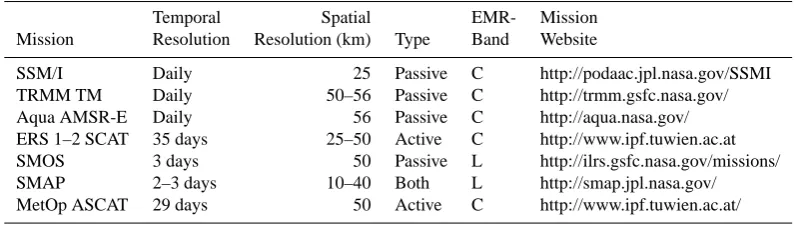
Table 1. Synopsis of recent and future satellite soil moisture missions.

Temporal Spatial EMR- Mission

Mission Resolution Resolution (km) Type Band Website

SSM/I Daily 25 Passive C http://podaac.jpl.nasa.gov/SSMI

TRMM TM Daily 50–56 Passive C http://trmm.gsfc.nasa.gov/

Aqua AMSR-E Daily 56 Passive C http://aqua.nasa.gov/

ERS 1–2 SCAT 35 days 25–50 Active C http://www.ipf.tuwien.ac.at

SMOS 3 days 50 Passive L http://ilrs.gsfc.nasa.gov/missions/

SMAP 2–3 days 10–40 Both L http://smap.jpl.nasa.gov/

MetOp ASCAT 29 days 50 Active C http://www.ipf.tuwien.ac.at/

soil moisture variability using the National Center for At-mospheric Research Community Climate Model, version 3 (NCAR CCM3). They found that correlations between the near-surface and root zone soil moisture vary seasonally. Wu et al. (2002) studied the variability of soil moisture observa-tions in Illinois and found that soil wetness influences how quickly soil wetting/drying moves through the soil column.

Mahmood and Hubbard (2007) used a soil-water energy balance model to examine the relationship between near-surface and root zone soil moisture in Nebraska. Their re-sults showed that cross correlations between near-surface and root zone soil moisture data sets exhibited high variability across Nebraska due to differences in soil, land use and cli-matic conditions. However, they concluded that it is possible to accurately estimate root zone soil moisture based on near-surface soil moisture. Mahmood et al. (2012) examined the predictability of soil moisture at various depths in Nebraska. They found that, in general, root zone soil moisture can be accurately estimated using 10 cm observations. However, es-timation accuracy depends on the prevailing climatological conditions. In general, predictions of root zone soil moisture are more accurate in locations that receive more precipitation (i.e., soils with higher water content) (Mahmood and Hub-bard, 2007; Mahmood et al., 2012). Overall, previous studies have suggested that soil moisture in the root zone is corre-lated with near surface soil moisture. Therefore, satellite soil moisture retrievals may provide an accurate means of esti-mating water content in the root zone.

In situ measurements of soil moisture are limited in their spatial and temporal extent (Prigent et al., 2005; Reichle and Koster, 2005). Satellites provide more extensive spa-tial coverage and have a temporal resolution ranging from 1 to 35+day(s). There are many different satellite missions that collect soil moisture data. Table 1 summarizes informa-tion about these satellite missions. The satellites assess soil wetness using either the C-band (4–8 GHz) or the L-band (1–2 GHz). Each of these platforms is currently in use, ex-cept for the SMAP (Soil Moisture Active Passive) mission, which is scheduled to launch in November 2014 and will provide global soil moisture measurements every 2–3 days (Entekhabi et al., 2010). The first satellite mission to

fo-cus primarily on the collection of soil moisture data was the Soil Moisture Ocean Salinity (SMOS) satellite (Kerr et al., 2010, 2012). The European Space Agency (ESA) launched the SMOS satellite in October 2010. SMOS uses microwave radiometry for estimating soil moisture (Kerr et al., 2010, 2012). L-band radiometry is achieved through 69 small an-tennae, resulting in a ground resolution of 50 km (Kerr et al., 2010, 2012).

Several studies have compared SMOS estimates to in situ soil moisture data. Jackson et al. (2012) used a set of rela-tively dense in situ soil moisture observation sites to validate SMOS retrievals over USDA Agricultural Research Service experimental watersheds. Their results showed that SMOS soil moisture estimates are in relatively good agreement with soil moisture observations. Al Bitar et al. (2012) compared SMOS soil moisture estimates with in situ soil moisture ob-servations from Soil Climate Network (SCAN) and SNOw-pack TELemetry (SNOTEL) observation network stations throughout several regions of the United States. The results of their node-to-node validation revealed that the accuracy of SMOS soil moisture estimates vary significantly from site to site. Collow et al. (2012) compared SMOS-derived soil moisture to in situ measurements in the US Great Plains to evaluate the accuracy of the satellite measurements. They concluded that evaluating SMOS is difficult due to the lack of uniform soil moisture measurements.

SMOS measures soil water content in the top few centime-ters and thus cannot directly determine root zone soil mois-ture conditions. Therefore, it is important to evaluate the de-gree of association between near-surface and root zone soil moisture when attempting to estimate root zone moisture us-ing satellite retrievals. Previous studies have estimated root zone soil moisture (or soil wetness index) using only sur-face observations. Root zone soil moisture has been esti-mated from satellite surface soil moisture retrievals from a number of different platforms, including the ERS (European remote sensing) scatterometer (Wagner et al., 1999; Ceballos et al., 2005) and ASCAT (advanced scatterometer; Albergel et al., 2009; Brocca et al., 2010, 2011, 2013). The recursive exponential filter has also been previously applied to both in situ and model-estimated soil moisture (Albergel et al., 2008;

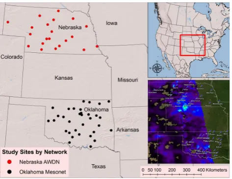
32

Figure 1. Soil moisture stations from the Nebraska Automated Weather Data Network and Oklahoma Mesonet that are used in this study. Automated Weather Data Network sites are red and Oklahoma Mesonet sites are dark blue. The lower right inset map shows a representative SMOS footprint from June 6, 2011 and the locations of stations in Oklahoma and Nebraska. Fig. 1. Soil moisture stations from the Nebraska Automated Weather Data Network and Oklahoma Mesonet that are used in this study. Automated Weather Data Network sites are red and Okla-homa Mesonet sites are dark blue. The lower right inset map shows a representative SMOS footprint from 6 June 2011 and the locations of stations in Oklahoma and Nebraska.

Barbu et al., 2011). Albergel et al. (2008) applies an exponen-tial filter to in situ soil moisture observations at a point scale and model estimates in France at a national scale. Albergel et al. (2010) compares the output of the exponential filter to soil moisture from a land data assimilation system at one site in southwestern France. The accuracy of these methods for de-riving root zone soil moisture estimates from SMOS have not been evaluated using North American soil moisture observa-tions. This study characterizes and quantifies the strength of the relationship between soil moisture in the near-surface and deeper soil and how it varies over time and space. In situ soil moisture observations over the North American Great Plains are used to calibrate an exponential filter model. This expo-nential filter is then employed to evaluate its utility for esti-mating root zone soil wetness from SMOS surface retrievals. The accuracy of the SMOS-derived estimates of root zone soil moisture are determined using observations from Okla-homa and Nebraska.

2 Data and methods

2.1 Study region

The North American Great Plains have a significant west– east precipitation gradient and north–south temperature gra-dient (Meng and Quiring, 2010). Vegetation and soil condi-tions exhibit great spatial variability across the region. Koster et al. (2004) characterize the southern Great Plains as a “hotspot” of land–atmosphere interactions. That is, this is a region where soil moisture and precipitation are strongly coupled. The southern Great Plains contains one of several

33

Figure 2. Mean monthly soil moisture (cm3_/cm3_{) in Oklahoma (top left) and Nebraska (bottom} left) and mean monthly coefficient of variation in Oklahoma (top right) and Nebraska (bottom right). Blue lines represent the near-surface soil (5 or 10 cm) while the green and red lines represent soil moisture at 20 or 25 cm and 50 or 60 cm, respectively.

Fig. 2. Mean monthly soil moisture (cm3cm−3) in Oklahoma (top left) and Nebraska (bottom left) and mean monthly coefficient of variation in Oklahoma (top right) and Nebraska (bottom right). Blue lines represent the near-surface soil (5 or 10 cm) while the green and red lines represent soil moisture at 20 or 25 cm and 50 or 60 cm, respectively.

SMAP test bed sites that are used to validate satellite soil moisture retrievals using in situ observations (Cosh et al., 2010). The Great Plains region was selected for this study because of the relatively high density of soil moisture obser-vations.

Daily volumetric soil water content estimates are from the Oklahoma Mesonet, www.mesonet.org, and Nebraska Au-tomated Weather Data Network (AWDN, http://www.hprcc. unl.edu/awdn/). The Oklahoma Mesonet operates more than 100 stations that measure meteorological variables on daily and sub-daily resolutions across Oklahoma (Illston et al., 2008). Volumetric soil water content is estimated at Okla-homa Mesonet sites from the matrix potential using Camp-bell Scientific 229-L sensors at 5, 25, 60 and 75 cm. The AWDN similarly operates meteorological stations across the northern Great Plains (You et al., 2010). AWDN estimates volumetric soil water content using Steven’s Hydra Probes placed at 10, 25, 50 and 100 cm in the soil column. The Ok-lahoma Mesonet soil moisture data analyzed span the pe-riod 2000–2012 and are at a daily resolution while AWDN data are available from 2006 to 2010 also at a daily res-olution. Volumetric water content data from 33 Oklahoma Mesonet sites and 22 AWDN sites are used in this study (Fig. 1). The sites were selected based on the length of record and completeness of the soil moisture data. All soil mois-ture data were quality controlled and distributed by the North American Soil Moisture Database at Texas A&M University (http://soilmoisture.tamu.edu).

2.2 Soil moisture data

Table 2 provides descriptive statistics of soil moisture in the near-surface (5 cm) and root zone (25 and 60 cm) averaged over all sites in Oklahoma. All values shown in Table 2 are in units of volumetric soil water content (cm3cm−3). In general soil moisture content in the near-surface correlates strongly

142 T. W. Ford et al.: Estimating root zone soil moisture

Table 2. Descriptive statistics for Oklahoma and Nebraska soil moisture. Table shows the mean, maximum, minimum, range and coefficient of variation (CV) averaged over all sites. All values are volumetric soil water content (cm3cm−3)units.

Oklahoma Nebraska

Average Maximum Minimum Average Maximum Minimum

Mean 5 cm 0.27 0.39 0.19 Mean 10 cm 0.19 0.32 0.07

Mean 25 cm 0.28 0.35 0.21 Mean 20 cm 0.19 0.35 0.07

Mean 60 cm 0.29 0.38 0.19 Mean 50 cm 0.20 0.35 0.07

Max 5 cm 0.32 0.48 0.21 Max 10 cm 0.30 0.43 0.13

Max 25 cm 0.33 0.42 0.24 Max 20 cm 0.29 0.43 0.10

Max 60 cm 0.33 0.42 0.22 Max 50 cm 0.29 0.42 0.11

Min 5 cm 0.20 0.28 0.16 Min 10 cm 0.07 0.17 0.02

Min 25 cm 0.21 0.28 0.16 Min 20 cm 0.08 0.25 0.00

Min 60 cm 0.23 0.30 0.17 Min 50 cm 0.10 0.24 0.02

Range 5 cm 0.13 0.26 0.05 Range 10 cm 0.22 0.32 0.10

Range 25 cm 0.12 0.23 0.05 Range 20 cm 0.21 0.31 0.09

Range 60 cm 0.10 0.18 0.05 Range 50 cm 0.19 0.28 0.09

CV 5 cm 0.14 0.25 0.05 CV 10 cm 0.32 0.47 0.17

CV 25 cm 0.13 0.22 0.07 CV 20 cm 0.29 0.43 0.09

CV 60 cm 0.12 0.20 0.06 CV 50 cm 0.28 0.48 0.08

with soil moisture at deeper layers. Average soil moisture content at Oklahoma sites is generally higher than at Ne-braska sites, while daily variability, as measured by the coef-ficient of variation (CV), is higher at the Nebraska sites. Soil moisture from both networks exhibits strong seasonal vari-ability. Figure 2 displays mean monthly soil moisture and CV for each network. Mean monthly soil moisture in Okla-homa peaks in early spring followed by drying throughout spring and summer. Soil moisture recharge occurs during the winter months. These patterns are similar to those reported by Illston et al. (2004). There is relatively little intra-annual variation in mean monthly CV, although soil moisture at 5 cm is consistently more variable than at 25 and 60 cm. Mean monthly soil moisture from Nebraska shows similar patterns to Oklahoma. However, the timing of the maximum and min-imum soil moisture is several weeks later in Nebraska. The period between March and May corresponds with lowest soil moisture variability in Nebraska.

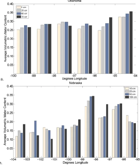
Soil moisture in Oklahoma and Nebraska also exhibits sig-nificant spatial variability. To characterize the west–east gra-dient in Great Plains soil moisture, driven by strong gragra-dients in precipitation, we binned Oklahoma and Nebraska stations according to their longitude. Figure 3 shows the mean volu-metric soil water content for (a) Oklahoma and (b) Nebraska. Stations in the eastern portion of both states generally ex-hibit higher average volumetric soil water content than those in the west. Mahmood et al. (2012) found that coupling be-tween root zone and near-surface soil moisture in Nebraska was stronger at locations with wetter climate/soils. Therefore we should expect to find stronger coupling between surface and root zone soil moisture at sites with wetter climatic con-ditions (eastern Oklahoma and eastern Nebraska).

34

a.

b.

Figure 3. Oklahoma Mesonet (a) and AWDN (b) stations are binned by the station's longitude. Bar graphs show the average volumetric soil water content for each bin at each measurement depth.

Fig. 3. Oklahoma Mesonet (a) and AWDN (b) stations are binned by the station’s longitude. Bar graphs show the average volumetric soil water content for each bin at each measurement depth.

35

. b.

c. d.

Figure 4. Sample cross correlations at two Oklahoma stations: (4a) and (4c) show 5-25 cm and 5-60 cm cross correlations at Durant, Oklahoma and (4b) and (4d) show 5-25 cm and 5-60 cm cross correlations at Miami, Oklahoma.

Fig. 4. Sample cross correlations at two Oklahoma stations: (a) and (c) show 5–25 cm and 5–60 cm cross correlations at Durant, Okla-homa and (b) and (d) show 5–25 cm and 5–60 cm cross correlations at Miami, Oklahoma.

2.3 Methods

Two methods used in previously published studies were em-ployed to characterize the relationship and coupling strength between near-surface and root zone layer soil moisture in Oklahoma and Nebraska (Albergel et al., 2008; Mahmood et al., 2012). The first method calculates lagged cross corre-lation coefficients between near-surface soil moisture obser-vations (at 5 or 10 cm) and those deeper in the soil (at 25 and 50 or 60 cm). Daily root zone soil moisture data is lagged 25 days with respect to the near-surface soil moisture data. Maximum lagged cross correlation coefficients between the two depths are evaluated as well as the lag time (in days) at which the maximum cross correlation was attained. Mah-mood et al. (2012) used a similar methodology when examin-ing the relationship between soil moisture at various depths in Nebraska. Cross correlation coefficients characterize the association between soil moisture in the near-surface and soil moisture in the root zone. When the correlations are small, this indicates that the near-surface and root zone are weakly coupled and therefore near-surface soil moisture has limited utility for predicting root zone soil moisture.

After examining the soil moisture coupling, we evaluate a method for inferring root zone soil moisture from near-surface observations. Previous studies have evaluated various forms of ensemble or extended Kalman filtering (Crow and Wood, 2003; Sabater et al., 2007; Draper et al., 2009; Hain et al., 2012) for estimating root zone soil moisture and land data assimilation for land surface models. For instance, Draper et al. (2009) found that the extended Kalman filter was useful for assimilating AMSR-E data into a land surface scheme. Li et al. (2012) employed a Kalman smoothing method to assimilate GRACE terrestrial water storage into the NASA catchment land surface model. In contrast, Hsu et al. (2012) found success employing a sequential Monte Carlo

particle-36

a. b.

c. d.

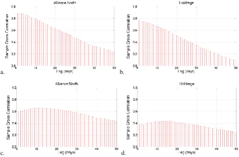
Figure 5. Sample cross correlations at two Nebraska stations: (4a) and (4c) show 10-25 cm and 10-50 cm cross correlations at Alliance North, Nebraska and (4b) and (4d) show 10-25 cm and 10-50 cm cross correlations at Holdrege, Nebraska.

Fig. 5. Sample cross correlations at two Nebraska stations: (a) and (c) show 10–25 cm and 10–50 cm cross correlations at Alliance North, Nebraska and (b) and (d) show 10–25 cm and 10–50 cm cross correlations at Holdrege, Nebraska.

filter technique to assimilate AMSR-E data into the Noah land surface model. These land data assimilation schemes are typically employed to correct soil moisture when measure-ments of root zone soil moisture are not available (Albergel et al., 2010). On the other hand, the exponential filter method estimates root zone soil moisture in areas where only surface soil moisture is available and this method is better suited for near-real time monitoring of soil moisture conditions.

In this study we evaluate the utility of the exponential fil-ter method described by Albergel et al. (2008) for estimat-ing root zone soil moisture from near-surface observations. The filter uses near-surface soil moisture observations and applies an exponential decay function to estimate root zone soil moisture. Previous studies have successfully employed similar methods to estimate root zone soil moisture in dif-ferent regions of the world and using various satellite plat-forms (Wagner et al., 1999; Albergel et al., 2009; Brocca et al., 2010). Our study evaluates the utility of this method for assimilating root zone soil moisture based on SMOS-derived surface soil moisture. The advantages of the exponential fil-ter method are that it is easy to implement and it is compu-tationally efficient. This method is particularly useful when only surface soil moisture data are available.

This study investigates three questions: (1) are surface and root zone soil moisture strongly related? (2) Can the ex-ponential filter be used to predict root zone soil moisture? (3) How accurate are SMOS-based estimates of root zone soil moisture derived using the exponential filter? The results sec-tion of this paper is organized around these three quessec-tions.

144 T. W. Ford et al.: Estimating root zone soil moisture

37 Figure 6. Peak cross correlation (r) between the 5 and 25 cm layers for all Oklahoma sites versus the average annual precipitation. Each point represents one site.

Fig. 6. Peak cross correlation (r) between the 5 and 25 cm layers for all Oklahoma sites versus the average annual precipitation. Each point represents one site.

3 Results

3.1 Cross correlation results

The 5–25 cm cross correlation in Durant and Miami, Okla-homa have pronounced peaks in strength with a∼5 day lag (Fig. 4a, b). Similar patterns are shown in 10–25 cm cross correlation plots for Alliance North and Holdrege, Nebraska (Fig. 5a, b). The cross correlations in the 5–60 cm (Fig. 4c, d) and 10–50 cm (Fig. 5c, d) are weaker and have lag times that are approximately 5–10 days longer.

Greater than 30 % of Oklahoma Mesonet soil moisture data at the 75 cm depth was missing, therefore we did not evaluate cross correlations at this depth. The maximum 5– 25 cm cross correlation at Oklahoma sites ranged from 0.62 to 0.95 with an overall average of 0.78. The lag times for 5– 25 cm ranged from 0 to 4 days with an overall average of 2 days. Not surprisingly, maximum 5–60 cm cross correlations were generally weaker than the 5–25 cm. This supports the findings of Wu et al. (2002) that coupling strength between soil layers decreases as depth increases. Maximum 5–60 cm cross correlations in Oklahoma ranged from 0.43 to 0.86 at Woodward, with an overall average of 0.61. The lag times for the 5–60 cm correlations were generally longer than the 5–25 cm and they ranged from 2 to 26 days. The decreases in cross correlation strength with depth agree with the findings of Mahmood et al. (2012).

Similar results were attained for stations in Nebraska, as the maximum cross correlation for 10–25 cm ranged from 0.66 to 0.88 with an overall average of 0.79. Lag times for the 10–25 cm cross correlations ranged from 0 to 5 days with an overall mean of 2 days. Maximum cross correlations for 10–50 cm ranged from 0.35 to 0.71 with an overall mean of 0.57. Lag times for the 10–50 cm cross correlations ranged from 1 day to 26 days with an overall mean of 8 days. Fi-nally, cross correlations between 10 and 100 cm ranged from 0.26 to 0.55 with an overall mean of 0.41. Lag times for the 10–100 cm cross correlations ranged from 1 to 87 days with

38 Figure 7. Peak cross correlation (r) between the 10 and 25 cm layers for all Nebraska sites versus the average annual precipitation. Each point represents one site. Fig. 7. Peak cross correlation (r) between the 10 and 25 cm layers

for all Nebraska sites versus the average annual precipitation. Each point represents one site.

an overall average of 33 days. Similar to the results from Ok-lahoma, cross correlations tend to decrease and lag times tend to increase as the depth increases.

We also calculated serial autocorrelation of daily near-surface soil moisture data at each Oklahoma and Ne-braska station. The majority of autocorrelation functions (not shown) show strong autocorrelation of surface soil moisture at timescales of 1–5 days, but significantly decreased au-tocorrelation strength after 10 days. This suggests that the strong cross correlation between surface and root zone soil layers is partly due to the strong serial autocorrelation of sur-face soil moisture. However, beyond a week, autocorrelation quickly decreases and cross correlations are more strongly a function of the coupling between soil layers.

3.2 Cross correlation strength–precipitation relationship

To assess the influence of precipitation on the strength of soil layer coupling, we created scatter plots of the aver-age annual precipitation, attained by the Parameter-elevation Regressions on Independent Slopes Model (PRISM) (http: //www.prism.oregonstate.edu/), with the peak cross correla-tion coefficient at each site. The relacorrela-tionship between pre-cipitation and the strength of the cross correlations between the near-surface (5 or 10 cm) and 25 cm soil moisture are shown in Figs. 6 and 7. In Oklahoma, there is a moderately strong positive relationship between the mean annual precipi-tation and 5–25 cm cross correlation coefficients (R2= 0.33). This suggests that wetter locations (eastern Oklahoma) tend to have stronger coupling between soil moisture in the near-surface and deeper in the soil. This is in agreement with pre-vious research (Mahmood and Hubbard, 2007; Mahmood et al., 2012). However, Fig. 7 shows that the relationship be-tween mean annual precipitation and 10–25 cm cross corre-lations in Nebraska are negative (R2 =0.27). Mahmood et al. (2012) found that cross correlations between the 10 and 50 cm soil moisture in Nebraska were stronger in wetter

locations. This is corroborated by our results in Oklahoma and contrasts with our results in Nebraska. The differences in the sign of the relationship between Nebraska and Oklahoma may be due to site-specific factors such as the near-surface depth of measurement (5 versus 10 cm) or soil texture. How-ever, we examined additional variables (soil texture, land cover, temperature) and were unable to determine why the relationship in Nebraska between cross correlation strength and mean annual precipitation is opposite of Oklahoma.

The cross correlation results suggest that associations be-tween near-surface and root zone soil moisture are strong at the majority of observation sites in Oklahoma and Nebraska. Our results and those of previous studies (Houser et al., 1998; Calvet and Noilham, 2000; Walker et al., 2001; Mahmood et al., 2012) suggest that it is possible to use surface soil mois-ture estimates (either from satellites or in situ measurements) to make skillful predictions of root zone soil moisture. There-fore, in the next section we evaluate the accuracy of root zone soil moisture estimates that are based on near-surface soil moisture observations.

3.3 Exponential filter

Albergel et al. (2008) used a recursive exponential filter to predict root zone soil moisture from near-surface observa-tions. The recursive formulation is used to predict the soil wetness index (SWI), a metric of soil moisture which stan-dardizes volumetric soil water content by the minimum and maximum values attained over the entire period of record at each location. The recursive equation adopted from Albergel et al., (2008) for predicting soil moisture at timetn, can be

written as

SWImn=SWIm(n−1)+Kn(ms(tn)−SWIm(n−1)), (1)

where SWIm(n−1)is the predicted root zone soil moisture

es-timate attn−1, ms(tn)is the surface soil moisture estimate at

tn, and the gainKat timetnis given by

Kn=

Kn−1

Kn−1+e−

tn−_tn−1

T

, (2)

whereT represents the timescale of soil moisture variation, in day units. The filter is initialized with SWIm(1)=ms(t1) andK1=1. Albergel et al. (2008) found that accuracy var-ied as a function of theT value. They showed that each study site had an optimal T value or Topt, which was character-ized by the highest prediction accuracy as assessed by the Nash–Sutcliffe score. We applied the filter to soil moisture in Oklahoma and Nebraska and assessed the accuracy of the root zone soil moisture estimates using several metrics in-cluding mean absolute error (MAE), mean bias error (MBE), the Nash–Sutcliffe score (NS) and the coefficient of determi-nation (R2). TheT parameter corresponding to the highest NS score was considered theToptfor that station.

39

a.

b.

Figure 8. Monthly average error metrics calculated from 5-25 cm soil moisture predictions. Results are averaged across all (a) Oklahoma and (b) Nebraska stations. Fig. 8. Monthly average error metrics calculated from 5 to 25 cm

soil moisture predictions. Results are averaged across all (a) Okla-homa and (b) Nebraska stations.

3.3.1 Overall results

Daily volumetric soil water content data are normalized (SWI) prior to the exponential filter. The SWI values are cal-culated using the maximum and minimum values from the entire daily volumetric water content time series (Oklahoma: 2000–2012, Nebraska: 2006–2010). Albergel et al. (2008) used 5 cm SWI to predict 30 cm SWI. Therefore, we applied this approach in Oklahoma by using daily 5 cm SWI to dict 25 cm SWI and in Nebraska we used 10 cm SWI to pre-dict 25 cm SWI.

NS values between estimated 25 cm SWI and observed 25 cm SWI ranged from 0.07 to 0.84 with an overall average of 0.63.R2values ranged from 0.52 to 0.91 with an overall average of 0.73. The optimumT parameter, orTopt, is defined as theT value at which the maximum observed–estimated root zone SWI NS score occurred for each station.Topt pa-rameter values ranged from 2 to 22 days with an overall av-erage of 8 days. Results were similar in Nebraska. NS values ranged from 0.08 to 0.83 with an overall average of 0.64.

R2values ranged from 0.51 to 0.84 with an overall average of 0.71.Topt parameter values for sites in Nebraska ranged from 3 to 20 days with an overall average of 9 days.

Root zone SWI predictions were generally accurate and, based on NS scores, all were more accurate than simply using

146 T. W. Ford et al.: Estimating root zone soil moisture

the mean root zone soil moisture as the prediction. Figure 8 shows plots of monthly average error metrics for (a) Okla-homa and (b) Nebraska. Root zone soil moisture estimates were generally higher than the soil moisture observations. Therefore, the mean bias (observed – predicted) is gener-ally negative. For example, in Oklahoma (Fig. 8a) the mean bias is negative, except for a brief period between July and September. This period coincides with increased error, which is probably due to the relatively low soil moisture values in the root zone during the late summer period. Figure 8a also shows a marked drop in NS between February and April, with an NS<0.3 in March. Illston et al. (2004) observed four distinct seasonal soil moisture regimes in Oklahoma. The transition between the first regime and second regime (February–April) is characterized by the initiation of 5 cm soil moisture drying beginning in mid-March, while 25 cm soil moisture drying does not initiate until early-to-mid April. This could be one factor influencing the relatively low ac-curacy when predicting 25 cm soil moisture from 5 cm soil moisture during this period.

Figure 8b shows monthly average error metrics from root zone soil moisture predictions in Nebraska. MAE and MBE are all relatively consistent across months; however,R2and NS values increase notably between April and May. Mah-mood et al. (2012) found that this period in Nebraska was characterized by soil moisture recharge at all depths. Their results also showed that coupling between 10 cm soil mois-ture and deeper (25, 50, 100 cm) soil moismois-ture was strongest under the wettest conditions. Predictions of root zone soil moisture from near-surface soil moisture should be most ac-curate during periods of soil moisture recharge.

3.3.2 OptimumT parameter

We found the station-specificTopt parameter for each Ok-lahoma and Nebraska site, based on maximum NS value. Similar to the results from Albergel et al. (2008) we found thatToptvaries considerably between stations. However, the monthly variability in NS shown in Fig. 9 suggests thatTopt could be a function of both space and time. Thus we quan-tified the influence of the overall soil moisture conditions on the variability ofTopt. To do this, we divided all of the near-surface SWI values from Oklahoma and Nebraska into 10 bins of equal range (0.0–0.1, 0.1–0.2, etc.). Each near-surface SWI observation was associated with a root zone soil moisture prediction and a corresponding NS value, measur-ing the accuracy of the prediction. We calculated the average NS value for each near-surface SWI bin. Figure 9 shows vari-ability of the NS score andToptparameter as a function of the near-surface SWI bin for sites in (a) Oklahoma and (b) Ne-braska, respectively.

The highest NS scores at Oklahoma sites (Fig. 9a) are all attained atTopt between 3 and 10 days. When SWI is be-tween 0.2 and 0.7, NS scores stay positive withToptvalues up to 40 days. However, when SWI is less than 0.2 or greater

40

a.

b.

Figure 9. Plots of the Nash-Sutcliffe score and the optimum T parameter as a function of the SWI conditions in the near-surface soil layer. Results are based on all of the (a) Oklahoma and (b) Nebraska sites.

Fig. 9. Plots of the Nash–Sutcliffe score and the optimumT pa-rameter as a function of the SWI conditions in the near-surface soil layer. Results are based on all of the (a) Oklahoma and (b) Nebraska sites.

than 0.7, NS scores quickly become negative whenToptis greater than 15–20 days. Like in Oklahoma sites, the highest NS at Nebraska sites occur atToptbetween 2 and 7 days. Ne-braska NS scores (Fig. 9b) also become negative when SWI is extremely dry (<0.1) or wet (>0.8) atToptgreater than 10 days. Therefore, the accuracy of the root zone soil moisture estimates are very sensitive to theToptparameter when over-lying near-surface soil moisture conditions are extremely dry or wet. Under more normal soil moisture conditions, the ac-curacy of the exponential filter method is nearly independent of theToptparameter.

Albergel et al. (2008) found that although Topt varied strongly between stations in their study, using the overall av-erageToptbased on all stations did not result in a significant decrease in model accuracy. We evaluated this finding in our study region by initializing the exponential filter model us-ing three different Topt parameters: (1) the overall average

Topt, which was 8 days for Oklahoma sites and 9 days for Nebraska sites, (2) site-specificToptparameters, and (3)Topt based on the near-surface SWI, ms(tn), conditions. Figure 10

shows box plots of the six error metrics calculated from the 3 differentToptparameters for (a) Oklahoma and (b) Nebraska sites, respectively. A paired Student’st test was used to de-termine if the soil moisture estimates generated using these

41

a.

b.

Figure 10. Box plots of error metrics for the estimated root-zone soil moisture averaged over all (a) Oklahoma and (b) Nebraska sites. Each boxplot is generated from estimates made with one of three different optimum T parameters.

Fig. 10. Box plots of error metrics for the estimated root zone soil moisture averaged over all (a) Oklahoma and (b) Nebraska sites. Each box plot is generated from estimates made with one of three different optimum T parameters.

three differentToptparameters were statistically significant. Figure 10a shows that using an averageToptvalue when pre-dicting root zone soil moisture values in Oklahoma does not result in significantly higher prediction error than using site-specific or ms(tn)-specific Topt parameters. Similar results are observed in Nebraska (Fig. 10b); the overall averageTopt parameter does not result in significantly higher error than the more dynamicToptvalues.

We found that a network-averageTopt parameter can be used with the exponential filter to accurately predict root zone soil moisture using near-surface observations. Our re-sults corroborate the findings of Albergel et al. (2008). We similarly assessed the variability of estimated soil moisture with a dynamicToptparameter using R2 instead of the NS score. The results were similar in thatToptparameter values of 8 and 9 days respectively resulted in the highestR2 val-ues. High levels of correspondence between assimilated root zone soil wetness and root zone observations are reported in several previous studies (Albergel et al., 2010; Barbu et al., 2011). Our results also show that the exponential filter method can accurately estimate root zone soil moisture in a different climatic regime (Great Plains) than the one in which it was developed and initially tested (Southern France).

4 Estimating root zone soil moisture using SMOS

Our results show that near-surface soil moisture is moder-ately to strongly coupled with soil moisture in the root zone (Sect. 3.2), and that near-surface SWI, based on observations, can be used to provide reasonably skillful predictions of root zone SWI (Sect. 3.3). Next we will evaluate the utility of the exponential decay filter for inferring root zone soil moisture from SMOS-derived surface soil moisture in Oklahoma and Nebraska. Once-daily SMOS surface retrievals between Jan-uary and December 2011 were collected over 23 Oklahoma Mesonet sites and 22 Nebraska AWDN sites.

4.1 Station–SMOS surface soil moisture comparison

The correspondence between SMOS surface retrievals and near-surface in situ soil moisture observations provides the “baseline” error against which we will compare the accuracy of the SMOS estimates of root zone soil moisture. Data from each in situ station were compared directly to SMOS, and the coefficient of determination (R2)and NS score were used to assess the relationship strength between the two data sets. Because of the scale differences between stations and the satellite footprint, all error metrics are based on SWI instead of raw volumetric water content. This ensures both data sets have the same mean and range of values, thus making error assessment solely based on co-variability of the data sets.R2

values in Oklahoma ranged from 0.32 to 0.71 with an overall mean of 0.56. The relationship between observed and SMOS SWI was significant (α= 0.05) at every Oklahoma station, in-dicating good correspondence between the two data sets. NS scores for the observed and SMOS SWI in Oklahoma ranged from 0.45 to 0.91, with an overall mean of 0.71. NS scores at all Oklahoma stations were positive, indicating good agree-ment between the two data sets.

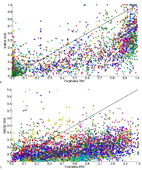
The correspondence between near-surface SWI observa-tions and SMOS SWI was similarly evaluated at staobserva-tions in Nebraska. NebraskaR2values ranged from 0.00 to 0.33, with an overall mean of 0.16. NS scores over Nebraska were also significantly lower than those over Oklahoma. NS values in Nebraska ranged from−1.82 to 0.60, with an overall mean of −0.48. NS scores were positive at only 4 of the 22 sta-tions in Nebraska. Clearly the relasta-tionship between observed SWI and SMOS SWI is stronger in Oklahoma than in Ne-braska. Figure 11 shows scatter plots between observed SWI and SMOS SWI at (a) Oklahoma and (b) Nebraska stations. Although both plots show substantial scatter around the 1-to-1 line, the data sets show better agreement in Oklahoma. There is evidence of a systematic bias in Nebraska. None of the days when the observed SWI in Nebraska was greater than 0.7 have a corresponding SMOS SWI greater than 0.7. The differences between Oklahoma and Nebraska suggest that the relationships between satellite soil moisture and in situ observations can vary significantly over space.

148 T. W. Ford et al.: Estimating root zone soil moisture

42

a.

b.

Figure 11. Scatter plots of observed near-surface SWI and SMOS surface SWI for (a) Oklahoma and (b) Nebraska stations. Scatter points are color coded by individual stations. Fig. 11. Scatter plots of observed near-surface SWI and SMOS sur-face SWI for (a) Oklahoma and (b) Nebraska stations. Scatter points are color coded by individual stations.

4.2 Station–SMOS root zone soil moisture comparison

The exponential decay filter described in Sect. 3.3 is used to estimate root zone soil moisture from the SMOS surface es-timates. Similar to results shown in Fig. 9, we varied theT

parameter from 1 to 25 days. Root zone SWI was estimated from SMOS surface data using eachT parameter. The per-formance of the filter under varyingT values was evaluated using the NS score, which was calculated based on compar-ing the root zone SWI estimated from SMOS with the in situ root zone SWI. Figure 12 shows how the accuracy of the esti-mated root zone SWI varies as a function of theT parameter. Figure 12a shows results from Oklahoma, where accuracy peaks at 8–10 days and begins to decline asTapproaches 25 days. Figure 12b shows results from Nebraska, where accu-racy consistently increases as theT parameter increases to 25 days. For both cases, the accuracy of the method using theTopt parameters derived from the in situ data sets (Ok-lahoma 8 days, Nebraska 9 days) is not substantially lower than the peak accuracy shown in Fig. 12. Therefore we used the originalToptparameter values to estimate root zone SWI using SMOS. Daily estimates of SMOS root zone SWI were compared to observed root zone SWI at stations in Oklahoma and Nebraska. Accuracy was measured using MAE, MBE,

R2and NS score.

43

a.

b.

Figure 12. Performance (NS score) of the exponential filter method when estimating root zone SWI from SMOS surface data as a function of T-parameter values. The top plot shows results for Oklahoma and the bottom shows results for Nebraska. NS scores are calculated between SMOS-estimated root zone soil moisture and in situ root zone soil moisture.

Fig. 12. Performance (NS score) of the exponential filter method when estimating root zone SWI from SMOS surface data as a func-tion of T-parameter values. The top plot shows results for Oklahoma and the bottom shows results for Nebraska. NS scores are calculated between SMOS-estimated root zone soil moisture and in situ root zone soil moisture.

4.2.1 SMOS results in Oklahoma

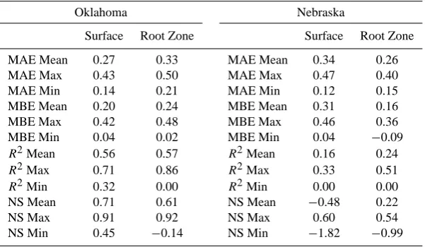
SMOS root zone SWI estimates are compared to observed 25 cm SWI at all stations in Oklahoma. The relationship be-tween SMOS surface retrievals and observed 5 cm soil mois-ture was used as the baseline by which to evaluate the SMOS root zone predictions. It can be used to determine how much of the error in the estimates of root zone SWI is due to the exponential filter method and how much is due to the uncer-tainties associated with the SMOS retrievals. Table 3 displays the overall mean, maximum and minimum values of MAE, MBER2, and NS score based on all of the stations in Okla-homa and Nebraska. All values in Table 3 are SWI (unitless).

R2 values ranged from 0.00 to 0.86 with an overall mean of 0.57. In general the correspondence between the two data sets is weaker at the root zone than at the surface. However,

R2values between root zone data are statistically significant at 20 of 22 Oklahoma stations. NS scores ranged from−0.14 to 0.92, with an overall mean of 0.61. NS scores at all but one Oklahoma stations are positive, indicating that there is good agreement between the observations and SMOS-based root zone SWI.

Table 3. Statistics showing the correspondence of SMOS and station SWI data sets. Values under surface are calculated from station surface– SMOS surface while values under root zone are calculated from station root zone – SMOS root zone. Table shows the mean, maximum and minimum over all sites. All values are SWI unitless.

Oklahoma Nebraska

Surface Root Zone Surface Root Zone

MAE Mean 0.27 0.33 MAE Mean 0.34 0.26

MAE Max 0.43 0.50 MAE Max 0.47 0.40

MAE Min 0.14 0.21 MAE Min 0.12 0.15

MBE Mean 0.20 0.24 MBE Mean 0.31 0.16

MBE Max 0.42 0.48 MBE Max 0.46 0.36

MBE Min 0.04 0.02 MBE Min 0.04 −0.09

R2Mean 0.56 0.57 R2Mean 0.16 0.24

R2Max 0.71 0.86 R2Max 0.33 0.51

R2Min 0.32 0.00 R2Min 0.00 0.00

NS Mean 0.71 0.61 NS Mean −0.48 0.22

NS Max 0.91 0.92 NS Max 0.60 0.54

NS Min 0.45 −0.14 NS Min −1.82 −0.99

44

a.

b.

Figure 13. The top plot shows MAE (SWI) at all Oklahoma stations. MAE is calculated between (blue circles) in situ surface observations and in situ root zone estimates, (green squares) in situ near-surface observations and SMOS surface retrievals and (red triangles) in situ root zone observations and SMOS root zone estimates. The bottom plot shows NS scores at all Oklahoma stations for the same dataset comparisons as in the top plot.

Fig. 13. The top plot shows MAE (SWI) at all Oklahoma stations. MAE is calculated between (blue circles) in situ surface observa-tions and in situ root zone estimates, (green squares) in situ near-surface observations and SMOS near-surface retrievals and (red trian-gles) in situ root zone observations and SMOS root zone estimates. The bottom plot shows NS scores at all Oklahoma stations for the same data set comparisons as in the top plot.

Partitioning error between the exponential filter and inher-ent SMOS-in situ differences gives a better description of where the largest discrepancies lie between observed and es-timated data. Figure 13a shows MAE values at all Oklahoma observation stations. Error is reported between (blue circles) in situ root zone observations and root zone SWI estimated from in situ observations using the exponential filter, (green squares) in situ surface observations and SMOS surface re-trievals, and (red triangles) in situ root zone observations and SWI estimated from SMOS using the exponential filter. At all but one Oklahoma station the MAE between SMOS surface retrievals and near-surface in situ observations was larger than the MAE between in situ root zone observations and root zone SWI estimated using the exponential filter. All but three stations had higher SMOS vs. observed root zone error than SMOS vs. observed surface error. On average, the SMOS–in situ surface comparison increased MAE by 0.13 (SWI) over Oklahoma in situ versus in situ root zone com-parison. Also SMOS–in situ root zone comparison increased MAE by 0.05 (SWI) over SMOS–in situ surface compari-son. This additional error represents roughly 20 % of average SMOS–in situ surface comparison error, suggesting that the inherent differences between the SMOS and in situ products are larger than error created by the exponential filter method. Regardless, the MAE between SMOS and in situ data sets represent on average 46 % of the observed mean SWI, and the exponential filter method increases the MAE to more than 50 % of the observation mean.

Figure 13b shows a similar plot to 13a, only it shows NS scores for the same three comparisons. On average, NS scores between SMOS and in situ surface SWI are 0.08 higher than NS scores between in situ root zone observations and in situ root zone estimates. In comparison, NS scores between SMOS root zone estimates and in situ root zone

150 T. W. Ford et al.: Estimating root zone soil moisture

45

Figure 14. Box plots of (left) volumetric water content at the 5 and 25 cm layers and (right) SWI from 25 cm in situ observations and 25 cm in situ estimates. The box plots show data from all Oklahoma stations.

Fig. 14. Box plots of (left) volumetric water content at the 5 and 25 cm layers and (right) SWI from 25 cm in situ observations and 25 cm in situ estimates. The box plots show data from all Oklahoma stations.

observations decrease on average by 0.09 as compared with SMOS–in situ surface NS scores. In general, direct SMOS– in situ comparisons lead to higher NS scores than comparing in situ observations to data sets estimated using the exponen-tial filter. This suggests that in Oklahoma, although inherent SMOS–in situ differences are larger than error created by the exponential filter method, these differences do not result in lower NS scores.

Results presented in this section exclude those from the Apache, Oklahoma station. MAE calculated from the expo-nential filter method applied to in situ observations were ex-ceptionally high, and NS scores were very low. Only when SMOS data were used did the MAE and NS scores resem-ble those from other Oklahoma stations. One issue with this station is the distribution of volumetric water content at the near-surface and root zone layers. Figure 14 shows box plots of (left) volumetric water content at the 5 and 25 cm layers, and (right) SWI calculated from 25 cm observations and esti-mated using the exponential filter method and 5 cm observa-tions. Clearly the mean and distribution of volumetric water content between the two soil layers are significantly differ-ent, as the 5 cm observations and 25 cm SWI estimates have a right-skewed distribution and the 25 cm observations (vol-umetric water content and SWI) have a left-skewed distri-bution. The difference in distributions is mostly attributable to soil texture differences between the 5 and 25 cm sensor locations. Apache soils in the top 5 cm are approximately 77 % sand content, corresponding to a saturated hydraulic conductivity of 213 cm day−1 _{(Scott et al., 2013). The soil} at 25 cm has a much lower sand content (∼20 % lower) and a higher clay content (10 % higher). Therefore, the sat-urated hydraulic conductivity is 73 cm day−1 at the 25 cm depth (Scott et al., 2013). Soil water moves through the near-surface layer relatively quickly, resulting in the right-skewed volumetric water content distribution (Fig. 14). While soil water content at 25 cm tends to be much higher because of the reduced hydraulic conductivity. This suggests that the ex-ponential filter method does not work well when soil textures

46 a.

b.

Figure 15. The top plot shows MAE (SWI) at all Nebraska stations. MAE is calculated between (blue circles) in situ surface observations and in situ root zone estimates, (green squares) in situ near-surface observations and SMOS surface retrievals and (red triangles) in situ root zone observations and SMOS root zone estimates. The bottom plot shows NS scores at all Nebraska stations for the same dataset comparisons as in the top plot.

Fig. 15. The top plot shows MAE (SWI) at all Nebraska stations. MAE is calculated between (blue circles) in situ surface observa-tions and in situ root zone estimates, (green squares) in situ near-surface observations and SMOS near-surface retrievals and (red trian-gles) in situ root zone observations and SMOS root zone estimates. The bottom plot shows NS scores at all Nebraska stations for the same data set comparisons as in the top plot.

are not homogenous in the soil column, and SMOS-based estimates of root zone soil moisture must take into account how soil characteristics vary with depth to produce accurate results.

4.2.2 SMOS results in Nebraska

The analysis from Sect. 4.2.1 was also applied at 22 stations in Nebraska.R2values between SMOS root zone SWI esti-mates and Nebraska root zone SWI observations ranged from 0.00 to 0.51, with an overall average of 0.24. Nebraska root zoneR2 values are larger than the surfaceR2values at all but 3 stations. Overall,R2values between root zone data sets are statistically significant at 18 sites. NS scores ranged from −0.99 to 0.54, with a mean of 0.22. NS scores at 18 Nebraska stations are positive, indicating good agreement between the observed and SMOS root zone SWI. NS scores for the root zone are higher than at the surface at 20 of 22 stations in Nebraska.

Figure 15a shows MAE values from all Nebraska stations, similar to Fig. 14a for Oklahoma stations. Blue circles rep-resent MAE between in situ root zone observations and es-timates from the exponential filter, green squares represent

T. W. Ford et al.: Estimating root zone soil moisture 151

47

Figure 16. Boxplots show mean bias error calculated from (left) surface SWI datasets and (right) root zone SWI datasets. MBE is calculated between Nebraska stations and SMOS data.

Figure 17. Boxplots show mean absolute error calculated from (left) surface SWI and (right) root zone SWI datasets. The left boxplot in each panel show MAE calculated over all months, while the right box plots in both panels show MAE calculated only during snow-free periods.

Fig. 16. Box plots show mean bias error calculated from (left) sur-face SWI data sets and (right) root zone SWI data sets. MBE is calculated between Nebraska stations and SMOS data.

MAE between in situ near-surface observations and SMOS surface retrievals and red triangles represent MAE between in situ root zone observations and SMOS root zone estimates. The differences (MAE) between SMOS and in situ obser-vations at the surface are greater than the differences when comparing SMOS and in situ in the root zone. This agrees with our findings in Oklahoma; however, MAE at Nebraska stations is decreased between SMOS surface comparisons and root zone comparisons. This contrasts with the results from Oklahoma (Fig. 14a) and it is counterintuitive because the exponential filter method is expected to introduce addi-tional error. Figure 16 shows the distribution of MBE be-tween (left) surface comparison and (right) root zone com-parison in Nebraska. All MBE values for the surface compar-ison are greater than zero, indicating that the observations are consistently wetter than SMOS. The MBE values in the root zone are much smaller. This indicates that the exponential fil-ter method reduces the differences between the observed and SMOS-based SWI values in the root zone and thus greatly decreases the error (MAE and MBE) with respect to the sur-face SWI comparison.

Figure 15b shows NS scores from all Nebraska stations. The NS scores between SMOS and in situ surface observa-tions are only positive at 3 out of 22 staobserva-tions. It is somewhat surprising that NS scores between SMOS retrievals and near-surface in situ observations are so low over Nebraska. One possible explanation is that Nebraska receives considerably more snow than Oklahoma between November and March. According to the National Weather Service’s National Op-erational Hydrologic Remote Sensing Center (NOHRSC), most of Nebraska was snow covered until the end of March, 2011, and then again starting at the beginning of November. To test if snow cover influences the accuracy of SMOS re-trievals, we examined the snow-free period (April–October). Figure 16 shows box plots of MAE between (left) SMOS surface retrievals and in situ near-surface observations and (right) SMOS root zone estimates and in situ root zone

ob-47 Figure 16. Boxplots show mean bias error calculated from (left) surface SWI datasets and (right) root zone SWI datasets. MBE is calculated between Nebraska stations and SMOS data.

Figure 17. Boxplots show mean absolute error calculated from (left) surface SWI and (right) root zone SWI datasets. The left boxplot in each panel show MAE calculated over all months, while the right box plots in both panels show MAE calculated only during snow-free periods.

Fig. 17. Box plots show mean absolute error calculated from (left) surface SWI and (right) root zone SWI data sets. The left box plot in each panel shows MAE calculated over all months, while the right box plots in both panels show MAE calculated only during snow-free periods.

servations at all Nebraska stations. For both plots, the left box shows the MAE distribution over all months, January– December, while the right box shows distributions between April and October. The mean surface MAE between January and December (0.33) is significantly higher than mean MAE between April and October (0.23). This suggests that SMOS soil moisture is more representative of observations during the growing season, particularly when there is no snow cover. However, the significant improvement in surface soil mois-ture accuracy does not translate to the root zone (Fig. 16), as there is no significant difference between SMOS root zone estimates and in situ root zone observations regardless of snow cover. Figure 17 compares the MAE values between in situ and SMOS at (left) the surface and (right) in the root zone for the snow-free period versus the entire year. MAE for the SMOS surface retrievals and in situ near-surface observa-tions are significantly lower between April and October than January–December, however there is not a significant MAE difference in the root zone.

After accounting for the influence of snow cover, the re-sults over Nebraska are similar to those over Oklahoma. In general the MAE of root zone estimates from the exponen-tial filter represent 10–20 % of the overall in situ SWI mean. In comparison, differences between SMOS surface retrievals and near-surface in situ observations represented 20–40 % of the overall in situ SWI mean. Despite the large MAE, NS scores at the majority of Nebraska stations are positive after accounting for snow cover.

Overall, the results from Oklahoma and Nebraska suggest that (1) the exponential filter can be a reasonably skillful method for estimating root zone soil moisture (mean error is ∼10 %) and (2) SMOS surface retrievals do not correspond well with in situ observations, but specifically for Nebraska, compatibility increases when only comparing SMOS over a land cover without snow. Our findings are generally in agree-ment with previous studies. Wagner et al. (1999) evaluated

152 T. W. Ford et al.: Estimating root zone soil moisture

root zone soil moisture estimates from ERS scatterome-ter data using multiple stations in Ukraine. The strength of correspondence between the satellite estimates and station-based observations was similar to our results. Ceballos et al. (2005) also found strong correlation (R2=0.75) between root zone soil wetness derived from ERS scatterometer sur-face retrievals and in situ observations over the semi-arid Duero Basin in Spain. Brocca et al. (2013) found strong correspondence between ASCAT-derived SWI and in situ soil moisture observations in northern Italy, withR2values exceeding 0.75.

5 Summary and conclusions

Satellite soil moisture retrievals are valuable because they provide better spatial coverage than in situ soil moisture ob-servations. SMOS measures soil water content in the top few centimeters and thus cannot directly determine root zone soil moisture conditions. Therefore, it is important to evaluate the degree of association between near-surface and root zone soil moisture when attempting to estimate root zone moisture using satellite retrievals. This study quantified the coupling strength between surface and root zone soil moisture. It also evaluated whether the exponential filter can be used to pre-dict root zone soil moisture. Finally, the accuracy of SMOS-based estimates of root zone soil moisture derived using the exponential filter were evaluated using in situ observations.

Cross correlation analysis was used to examine the re-lationship strength between near-surface and root zone soil moisture at 33 sites in Oklahoma and 22 sites in Nebraska. The results revealed generally strong relationships between soil moisture in the near-surface and root zone. However, the lag time at which the two layers correlated most strongly varied depending on climatic conditions. After the strong as-sociation between near-surface and root zone soil moisture was established, an exponential filter method from Albergel et al. (2008) was used to estimate root zone soil moisture based on near-surface observations. This method was shown to have skill. However, accuracy diminished during times of transition between soil moisture recharge (wet) and utiliza-tion (dry) phases. The primary coefficient of the exponential filter (Topt)was sensitive to soil wetness and varied consid-erably based on the climatic regime. The exponential filter method also did not perform well when soil characteristics varied considerably with depth.

The exponential filter method was used to estimate root zone soil moisture based on SMOS surface retrievals. The root zone estimates were compared to 25 cm soil moisture observations. SMOS root zone soil wetness and in situ root zone observations in Oklahoma and Nebraska show good correspondence, with R2 exceeding 0.90 at several sites. Specifically root zone soil moisture estimated using the ex-ponential filter did not correlate well with root zone obser-vations when the distributions of in situ volumetric water

content at the near-surface and root zone are different; as in Apache, Oklahoma. SMOS correspondence with in situ observations varied, but in general resulted in positive NS scores. SMOS corresponded most strongly with in situ ob-servations when the land surface was free of snow cover.

The main conclusions of this study are (1) soil moisture in near-surface and root zone layers in Oklahoma and Nebraska are strongly coupled, (2) the exponential filter method can provide accurate estimates of root zone soil moisture as long as soil characteristics are relatively homogeneous through-out the soil column and (3) SMOS surface soil moisture re-trievals can be used with the exponential filter method to es-timate root zone soil moisture over Oklahoma and Nebraska with reasonable skill, except when there is snow cover.

Acknowledgements. This research was funded by the National Science Foundation (award AGS-1056796). We would also like to acknowledge data provided by the Oklahoma Mesonet and Automated Weather Data Network for in situ soil moisture.

Edited by: N. Verhoest

References

Albergel, C., Rüdiger, C., Pellarin, T., Calvet, J.-C., Fritz, N., Frois-sard, F., Suquia, D., Petitpa, A., Piguet, B., and Martin, E.: From near-surface to root-zone soil moisture using an exponential fil-ter: an assessment of the method based on in-situ observations and model simulations, Hydrol. Earth Syst. Sci., 12, 1323–1337, doi:10.5194/hess-12-1323-2008, 2008.

Albergel, C., Rüdiger, C., Carrer, D., Calvet, J.-C., Fritz, N., Naeimi, V., Bartalis, Z., and Hasenauer, S.: An evaluation of ASCAT surface soil moisture products with in-situ observations in Southwestern France, Hydrol. Earth Syst. Sci., 13, 115–124, doi:10.5194/hess-13-115-2009, 2009.

Albergel, C., Calvet, J.-C., Mahfouf, J.-F., Rüdiger, C., Barbu, A. L., Lafont, S., Roujean, J.-L., Walker, J. P., Crapeau, M., and Wigneron, J.-P.: Monitoring of water and carbon fluxes us-ing a land data assimilation system: a case study for south-western France, Hydrol. Earth Syst. Sci., 14, 1109–1124, doi:10.5194/hess-14-1109-2010, 2010.

Al Bitar, A., Leroux, D., Kerr, Y. H., Merlin, O., Richaume, P., Sahoo, A., and Wood, E. F.: Evaluation of SMOS soil mois-ture products over continental US using the SCAN/SNOTEL net-work. Geoscience and Remote Sensing, IEEE Trans., 50, 1572– 1586, 2012.

Alfieri, L., Claps, P., D’Odorico, P., Laio, F., and Over, T. M.: An analysis of the soil moisture feedback on convective and strati-form precipitation, J. Hydrometeorol., 9, 280–291, 2008. Barbu, A. L., Calvet, J.-C., Mahfouf, J.-F., Albergel, C., and Lafont,

S.: Assimilation of Soil Wetness Index and Leaf Area Index into the ISBA-A-gs land surface model: grassland case study, Bio-geosciences, 8, 1971–1986, doi:10.5194/bg-8-1971-2011, 2011. Basara, J. B. and Crawford, K. C.: Linear relationships be-tween root-zone soil moisture and atmospheric processes in the planetary boundary layer, J. Geophys. Res., 107, 4274, doi:10.1029/2001JD000633, 2002.

Brocca, L., Melone, F., Moramarco, T., Wagner, W., Naeimi, V., Bartalis, Z., and Hasenauer, S.: Improving runoff prediction through the assimilation of the ASCAT soil moisture product, Hydrol. Earth Syst. Sci., 14, 1881–1893, doi:10.5194/hess-14-1881-2010, 2010.

Brocca, L., Hasenauer, S., Lacava, T., Melone, F., Moramarco, T., Wagner, W., Dorigo, W., Matgen, P., Martínez-Fernándz, J., Llorens, P., Latron, J., Martin, C., and Bittelli, M.: Soil moisture estimation through ASCAT and AMSR-E sensors: An intercom-parison and validation study across Europe, Remote Sens. Envi-ron., 115, 3390–3408, 2011.

Brocca, L., Tarpanelli, A., Moramarco, T., Melone, F., Ratto, S. M., Cauduro, M., Ferraris, S., Berni, N., Ponziani, F., Wagner, W., and Melzer, T.: Soil moisture estimation in alpine catchments through modeling and satellite observations, Vadose Zone Hy-drol., 12, 1–10, 2013.

Calvet, J. and Noilham, J.: From near-surface to root-zone soil moisture using year-round data. J. Hydrometeo. 1, 393–411, 2000.

Ceballos, A., Scipal, K., Wagner, W., and Martínez-Fernández, J.: Validation of ERS scatterometer-derived soil moisture data in the central part of the Duero Basin, Spain, Hydrol. Process., 19, 1549–1566, 2005.

Collow, T. W., Robock, A., Basara, J. B., and Illston, B. G.: Evalu-ation of SMOS retrievals of soil moisture over the central United States with currently available in situ observations, J. Geophys. Res., 117, D09113, doi:10.1029/2011JD017095, 2012.

Cosh, M. H., Ochsner, T., Basara, J., and Jackson, T. J.: The SMAP in situ soil moisture sensor testbed: Comparing in situ sensors for satellite validation, in: Geoscience and Remote Sensing Sympo-sium (IGARSS), 2010 IEEE International, 2010.

Crow, W. T. and Wood, E. F.: The assimilation of remotely sensed soil brightness temperature imagery into a land surface model using ensemble Kalman filtering: A case study based on ESTAR measurements during SGP97, Adv. Water Resour., 26, 137–149, 2003.

Draper, C., Mahfouf, J., and Walker, J.: An EKF assimilation of AMSR-E soil moisture into the ISBA land surface scheme, J. Geophys. Res.-Atmos., 114, 1984–2012, 2009.

Entekhabi, D., Nioku, E. G., O’Neill, P. E., Kellogg, K. H., Crow, W. T., Edelstein, W. N., Entin, J. K., Goodman, S. D., Jackson, T. J., Johnson, J., Kimball, J., Piepmeier, J. R., Koster, R. D., Mar-tin, N., McDonald, K. C., Moghaddam, M., Moran, S., Reichle, R., Shi, J.-C., Spencer, M. W., Thurman, S. W., Leung, T., and Van Zyl, J.: The Soil Moisture Active Passive (SMAP) Mission, Proc. IEEE., 98, 704–716, 2010.

Frye, J. D. and Mote, T. L.: Convection initiation along soil moisture boundaries in the southern Great Plains, Mon. Weather Rev., 138, 1140–1151, 2010.

Georgakakos, K. P. and Bae, D.: Climatic variability of soil water in the American Midwest: Part 2. Spatio-temporal analysis, J. Hydrol., 162, 379–390, 1994.

Hain, C. R., Crow, W. T., Anderson, M. C., and Mecikalski, J. R.: An ensemble Kalman filter dual assimilation of thermal in-frared and microwave satellite observations of soil moisture into the Noah land surface model, Water Resour. Res., 48, W11517, doi:10.1029/2011WR011268, 2012.

Houser, P. R., Shuttleworth, W. J., Famiglietti, J. S., Gupta, H. V., Syed, K. H., and Goodrich, D. C.: Integration of soil moisture remote sensing and hydrologic modeling using data assimilation, Water Resour. Res. 34, 3405–3420, 1998.

Hsu, K., Li, J., and Sorooshian, S.: To improve model soil mois-ture estimation in arid/semi-arid region using in situ and remote sensing information, Paddy Water Environ., 10, 165–173, 2012. Illston, B. G., Basara, J. B., and Crawford, K. C.: Seasonal to

inter-annual variations of soil moisture measured in Oklahoma, Int. J. Climatol., 24, 1883–1896, 2004.

Illston, B. G., Basara, J. B., Fiebrich, C. A., Crawford, K. C., Hunt, E., Fisher, D. K., Elliott, R., and Humes, K.: Mesoscale monitor-ing of soil moisture across a statewide network, J. Atmos. Ocean. Technol., 25, 167–182, 2008.

Jackson, T. J., Bindlish, R., Cosh, M. H., Zhao, T., Starks, P. J., Bosch, D. D., Seyfried, M., Moran, M. S., Goodrich, D. C., and Kerr, Y. H.: Validation of Soil Moisture and Ocean Salin-ity (SMOS) soil moisture over watershed networks in the US. Geoscience and Remote Sensing, IEEE Trans., 50, 1530–1543, 2012.

Kerr, Y. H., Waldteufel, P., Wigneron, J.-P., Delwart, S., Cabot, F., Boutin, J., Escorihuela, M.-J., Font, J., Reul, N., Gruhier, C., Ju-glea, S. E., Drinkwater, M. R., Hahne, A., Martin-Neira, M., and Mecklenburg, S.: The SMOS mission: New tool for monitoring key elements of the global water cycle, IEEE Trans., 98, 666– 687, 2010.

Kerr, Y. H., Waldteufel, P., Richaume, P., Wigneron, J.-P., Ferraz-zoli, P., Mahmoodi, A., Al Bitar, A., Cabot, F., Gruhier, C., Juglea, S. E., Leroux, D., Mialon, A., and Delwart, S.: The SMOS soil moisture retrieval algorithm, Geosci. Remote Sens., 50, 1384–1403, 2012.

Koster, R. D., Dirmeyer, P. A., Guo, Z., Bonan, G., Chan, E., Cox, P., Gordon, C., Kanae, S., Kowalczyk, E., and Lawrence, D.: Re-gions of strong coupling between soil moisture and precipitation, Science, 305, 1138–1140, 2004.

Legates, D. R., Mahmood, R., Levia, D. F., DeLiberty, T. L., Quir-ing, S. M., Houser, C., and Nelson, F. E.: Soil moisture: A central and unifying theme in physical geography, Prog. Phys. Geogr., 35, 65–86, 2011.

Li, B., Rodell, M., Zaitchik, B. F., Reichle, R. H., Koster, R. D., and van Dam, T. M.: Assimilation of GRACE terrestrial water storage into a land surface model: evaluation and potential value for drought monitoring in western and central Europe, J. Hydrol., 446–447, 103–115, 2012.

Mahmood, R. and Hubbard, K. G.: An analysis of simulated long-term soil moisture data for three land uses under contrasting hy-droclimatic conditions in the Northern Great Plains, J. Hydrom-eteorol., 5, 160–179, 2004.

Mahmood, R. and Hubbard, K. G.: Relationship between soil mois-ture of near surface and multiple depths of the root zone under heterogeneous land uses and varying hydroclimatic conditions, Hydrol. Process., 21, 3449–3462, 2007.

Mahmood, R., Littell, A., Hubbard, K. G., and You, J.: Observed data-based assessment of relationships among soil moisture at various depths, precipitation, and temperature, Appl. Geogr., 34, 255–264, 2012.

McPherson, R. A.: A review of vegetation-atmosphere interactions and their influences on mesoscale phenomena, Prog. Phys. Ge-ogr., 31, 262–285, 2007.

154 T. W. Ford et al.: Estimating root zone soil moisture

Meng, L. and Quiring, S. M.: Observational relationship of sea sur-face temperatures and precedent soil moisture with summer pre-cipitation in the US Great Plains, Int. J. Climatol., 30, 884–893, 2010.

Pal, J. S. and Eltahir, E. A. B.: Pathways relating soil moisture conditions to future summer rainfall within a model of the land-atmosphere system, 2001.

Prigent, C., Aires, F., Rossow, W. B., and Robock, A.: Sensitivity of satellite microwave and infrared observations to soil moisture at a global scale: Relationship of satellite observations to in situ soil moisture measurements, J. Geophys. Res.-Atmos., 110, 1984– 2012, 2005.

Reichle, R. H. and Koster, R. D.: Global assimilation of satel-lite surface soil moisture retrievals into the NASA Catch-ment land surface model, Geophys. Res. Lett., 32, L02404, doi:10.1029/2004GL021700, 2005.

Sabater, J. M., Jarlan, L., Calvet, J., Bouyssel, F., and De Rosnay, P.: From near-surface to root-zone soil moisture using different assimilation techniques, J. Hydrometeorol., 8, 194–206, 2007. Taylor, C. M., Parker, D. J., and Harris, P. P.: An

observa-tional case study of mesoscale atmospheric circulations in-duced by soil moisture, Geophys. Res. Lett., 34, L15801, doi:10.1029/2007GL030572, 2007.

Taylor, C. M., de Jeu, R. A., Guichard, F., Harris, P. P., and Dorigo, W. A.: Afternoon rain more likely over drier soils, Nature, 489, 423–426, 2012.

Wagner, W., Lemoine, G., and Rott, H.: A method for estimat-ing soil moisture from ERS scatterometer and soil data, Remote Sens. Environ., 70, 191–207, 1999.

Walker, J. P., Willgoose, G. R., and Kalma, J. D.: One-dimensional soil moisture profile retrieval by assimilation of near-surface measurements: A simplified soil moisture model and field ap-plication, J. Hydrometerol., 2, 356–373, 2001.

Wu, W. and Dickinson, R. E.: Time Scales of Layered Soil Mois-ture Memory in the Context ofLand-Atmosphere Interaction, J. Climate, 17, 2752–2764, 2004.

Wu, W., Geller, M. A., and Dickinson, R. E.: The response of soil moisture to long-term variability of precipitation, J. Hydromete-orol., 3, 604–613, 2002.

You, J., Hubbard, K. G., Mahmood, R., Sridhar, V., and Todey, D.: Quality Control of Soil Water Data in Applied Climate Infor-mation System – Case Study in Nebraska, J. Hydrol. Eng., 15, 200–209, 2010.