Precipitation bias correction of very high resolution regional climate models

Hydrol. Earth Syst. Sci., 17, 4379–4388, 2013 www.hydrol-earth-syst-sci.net/17/4379/2013/ doi:10.5194/hess-17-4379-2013

© Author(s) 2013. CC Attribution 3.0 License.

Hydrology and

Earth System

Sciences

Open Access

Precipitation bias correction of very high resolution regional climate

models

D. Argüeso1,2, J. P. Evans1,2, and L. Fita1,2

1_{Climate Change Research Centre, University of New South Wales, Sydney, NSW 2052, Australia}

2_{ARC Centre of Excellence for Climate System Science, University of New South Wales, Sydney, NSW 2052, Australia}

Correspondence to: D. Argüeso (d.argueso@unsw.edu.au)

Received: 21 May 2013 – Published in Hydrol. Earth Syst. Sci. Discuss.: 25 June 2013 Revised: 12 September 2013 – Accepted: 3 October 2013 – Published: 6 November 2013

Abstract. Regional climate models are prone to biases in precipitation that are problematic for use in impact models such as hydrology models. A large number of methods have already been proposed aimed at correcting various moments of the rainfall distribution. They all require that the model produce the same or a higher number of rain days than the observational data sets, which are usually gridded data sets. Models have traditionally met this condition because their spatial resolution was coarser than the observational grids. But recent climate simulations use higher resolution and the models are likely to systematically produce fewer rain days than the gridded observations.

In this study, model outputs from a simulation at 2 km res-olution are compared with gridded and in situ observational data sets to determine whether the new scenario calls for re-vised methodologies. The gridded observations are found to be inadequate to correct the high-resolution model at daily timescales, because they are subjected to too frequent low intensity precipitation due to spatial averaging. A histogram equalisation bias correction method was adapted to the use of station, alleviating the problems associated with relative low-resolution observational grids. The wet-day frequency condition might not be satisfied for extremely dry biases, but the proposed approach substantially increases the applicabil-ity of bias correction to high-resolution models. The method is efficient at bias correcting both seasonal and daily charac-teristic of precipitation, providing more accurate information that is crucial for impact assessment studies.

1 Introduction

Regional climate models (RCMs) are outstanding tools for studying the mechanisms of climate at scales that are not yet resolved by general circulation models (GCMs). Higher spa-tial resolution and specifically designed parameterizations of RCMs improve the representation of many aspects of climate (Feser et al., 2011; Giorgi, 2006), especially variables that are essentially local such as precipitation (Di Luca et al., 2011; Evans and McCabe, 2010; Tselioudis et al., 2012). Hydrological models, which are especially sensitive to pre-cipitation, thus benefit from high-resolution RCM outputs (Maraun et al., 2010).

However, RCMs are still prone to biases and the simu-lated climate is not always fully consistent with the obser-vations, which is critical in climate change impact research (Portoghese et al., 2011). Previous authors (Christensen et al., 2008; Déqué et al., 2007) have advocated the use of bias correction to reduce model systematic deviations and provide more reliable outputs. It is arguable that bias cor-rection should not be regarded as a definitive solution and its application is also matter of criticism (Ehret et al., 2012). Despite the fact that efforts should indeed be devoted towards the development of better models, there are no feasible alter-natives to bias correction in terms of improving current sim-ulations. Furthermore, some authors have examined the un-certainty introduced by bias correction and its impact on cli-mate change esticli-mates and overall recommended the use of non-linear methods to provide better projections (Chen et al., 2011; Themeßl et al., 2012).

(Berg et al., 2012; Bordoy and Burlando, 2013; Haerter et al., 2011; Piani et al., 2010a; Terink et al., 2010). The physi-cal characteristics of precipitation make it more difficult to correct and most studies tend to concentrate on precipita-tion correcprecipita-tion. Methods of different complexity have been put forward, aimed at correcting various moments of the rainfall distribution. They range from relatively simple lin-ear methods (Hay et al., 2000; Lenderink et al., 2007) to distribution-based algorithms, either using empirical distri-butions (Themeßl et al., 2011) or theoretical functions (Piani et al., 2010a). Hydrological impact studies require at least ac-curate daily data and hence methods that correct higher mo-ments are preferable (Portoghese et al., 2011). Several eval-uations (Lafon et al., 2013; Teutschbein and Seibert, 2012; Themeßl et al., 2011) have shown that distribution-mapping methods generally outperform others.

Bias correction is normally performed towards gridded data sets such as E-OBS (Haylock et al., 2008) or AWAP (Jones et al., 2009), because they cover the entire spatial do-main and have complete time series. The spatial compati-bility of gridded observations and model outputs of similar horizontal resolution has also been a reason to use gridded products in model bias correction. Both the model outputs and the gridded data set are reduced to the same grid and the transfer functions are calculated grid-point by grid-point.

No matter which method is selected among the myriad proposed, they all impose a common limitation to provide ac-curate corrections: they assume that the model produces the same or a higher number of rain days, independently from how these are defined. Distribution-based methods do not strictly require an equal or larger number of wet days, but if the model is generating too few rain days, the method might fail to adequately correct the model outputs. If any method is to be applied to model output with fewer rain days, it is necessary to introduce additional precipitation events (e.g. through Frequency Adaptation as in Themeßl et al., 2012) otherwise daily intensity might be unrealistically corrected to match, for example, the monthly means.

So far this situation has rarely arisen and RCMs have tra-ditionally met the aforementioned condition, partly because their spatial resolution is coarser than the observational grid-ded data set to which they are compared. Models often dis-play an increase in low intensity precipitation as a function of spatial resolution due to various reasons (i.e. model physics, spatial representativeness), producing more frequent but less intense precipitation than the station measurement as the res-olution decreases. Gridded observations are also affected by similar behaviour, mostly due to the gridding methodology that involves some sort of spatial averaging. RCM simula-tions that exceed the spatial resolution of most gridded prod-ucts have become possible due to improvements in computa-tional resources. Such RCMs are likely to produce systemati-cally less rain days than the gridded observations and thus the existing bias correction methodologies have to be revised.

In this paper, we analysed a RCM simulation at 2 km spa-tial resolution and compared it with both gridded and station based in situ observational data sets to determine whether increasing resolution has implications in terms of the bias correction. We propose an alternative approach to the use of gridded observations for this purpose.

2 Model and observational data

2.1 Model description and set-up

The Weather Research and Forecasting (WRF) model ver-sion 3.3.1 (Skamarock et al., 2009) was selected to simu-late the recent climate (1990–2009) over the Sydney region (Fig. 1a). The model was configured following Evans and McCabe (2010, 2013); Evans and Westra (2012), where thor-ough evaluations of WRF over the region are provided cov-ering timescales from sub-daily to inter-annual. The origi-nal simulation comprised two domains at 50 and 10 km spa-tial resolution covering southeastern Australia. The boundary conditions were obtained from the National Centers for En-vironmental Prediction (NCEP)/National Center for Atmo-spheric Research (NCAR) Reanalysis Project (NNRP1) and are provided every 6 h to the model.

An additional 2 km spatial resolution domain (Fig. 1) that covers the Sydney region was added to the original config-uration (Argüeso et al., 2013). The convective parameteri-zation was switched off in this domain, while the micro-physics parameterization was changed to the more complex Thompson scheme (Thompson et al., 2006).

2.2 Observational data

D. Argüeso et al.: High-resolution RCM precipitation bias correction 4381

Discussion

P

ap

er

|

Dis

cussion

P

ap

er

|

Discussion

P

ap

e

r

|

Discussion

P

ap

er

|

Fig. 1.

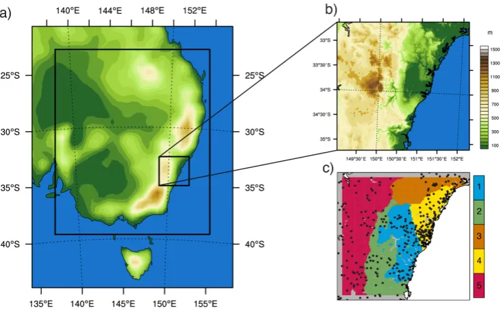
(a) Topography and location of all domains of the simulation, (b) topography and extension of

the inner domain, and (c) location of the stations (black dots) and the 5 different precipitation regions

(colored areas) within the model domain.

18

Fig. 1. (a) Topography and location of all domains of the simulation, (b) topography and extension of the inner domain, and (c) location of

the stations (black dots) and the 5 different precipitation regions (colored areas) within the model domain.

3 A methodology for the new paradigm

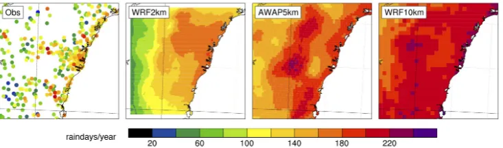
Existing methods usually perform the bias correction grid-point by grid-grid-point and assume that the model produces too many rain events. However, the respective number of wet days, defined as days with any precipitation registered, tends to decrease with resolution as evidenced by Fig. 2 and thus that assumption is unlikely to be valid for the increasingly high-resolution simulations being performed now and in the future. Indeed, the 2 km WRF simulation produces many less rain days than AWAP and therefore using the gridded data set to correct the 2 km model outputs is problematic. As men-tioned before, introducing new rain days to match the ob-served frequency poses a number of problems (i.e. when to introduce them, what is their intensity, how to keep spatial coherence) that encourages the proposal of alternatives.

Because the number of rain days decreases with increas-ing resolution the question that arises is why is station data not used directly to correct very high-resolution model out-puts? There are two major obstacles that explain why bias correction has not traditionally been carried out based on in situ measurements: (1) spatial and temporal coverage and, (2) discrepancies in the spatial scale represented by models and stations. Spatial discrepancies are reduced with higher reso-lution, but it remains a burden when comparing stations and model outputs. The coverage is still an issue regardless of the model spatial resolution and hence a good quality network is necessary. However, even the use of in situ observation does not guarantee that the model will have higher rain-day fre-quency and the biases in the number of wet days must still be calculated to ensure that the assumption is valid.

A completely new method is not necessary given the large number of bias correction methodologies that have already been proposed and proven to provide satisfactory results. In-stead, we suggest here an alternative approach aimed at over-coming the two obstacles above, which consists in adapting an existing method based on histogram equalisation (Piani et al., 2010a, b) to the use of stations as observational refer-ence. This method was chosen among a wide range of op-tions available because it is widely adopted (Lafon et al., 2013; Piani and Haerter, 2012; Rojas et al., 2011; Schoetter et al., 2012), corrects high moments of the distribution and performs generally better than others (Berg et al., 2012; Teutschbein and Seibert, 2012). Here we call attention to a problem that is likely to emerge in future simulations as res-olution increases, and offer a sres-olution.

The original method proposed in Piani et al. (2010a) is a distribution-based algorithm, which assumes that the prob-ability distribution of both the observed and the simulated daily rainfall could be approximated by a theoretical func-tion, a gamma distribution. In particular, the algorithm calcu-lates the cumulative probability from each of the theoretical distributions (i.e. from the model and the observations) at ev-ery grid-point. It then corrects each of the modelled rainfall intensities towards the observed value to match their respec-tive cumularespec-tive probabilities (Fig. 3). Therefore, provided that Fm andFo are the gamma functions that approximate

the model and the observations at a particular location, for a given event in the model (Mi) the theoretical cumulative probability (CPi_m) is calculated as

4382 D. Argüeso et al.: High-resolution RCM precipitation bias correction

P

ap

er

|

Dis

cussion

P

ap

er

|

Discussion

P

ap

e

r

|

Discussion

P

ap

er

|

Fig. 2.

Annual mean number of rain days over the period 1990-2009 for stations, the WRF simulation

at 2-km resolution, the AWAP dataset and the intermediate WRF domain at 10-km resolution used to

provide the boundary conditions.

19

Fig. 2. Annual mean number of rain days over the period 1990–2009 for stations, the WRF simulation at 2 km resolution, the AWAP data set

and the intermediate WRF domain at 10 km resolution used to provide the boundary conditions.

Discussion

P

ap

er

|

Dis

cussion

P

ap

er

|

Discussion

P

ap

e

r

|

Discussion

P

ap

er

|

Fig. 3.(a) Schematic of the bias correction proposed by Piani et al. (2010a). Mi is the intensity of an event in the model and Oi is intensity of an observed event with the same cumulative probability (CPmi) as defined by Fm and Fo, which are the cumulative probability functions for the model and the observations. (b) Schematic of the adaptation of the bias-correction method using stations and regions.

20

Fig. 3. (a) Schematic of the bias correction proposed by Piani et

al. (2010a). Mi is the intensity of an event in the model and Oi is intensity of an observed event with the same cumulative probability (CPmi) as defined by Fm and Fo, which are the cumulative proba-bility functions for the model and the observations. (b) Schematic of the adaptation of the bias-correction method using stations and regions.

then the inverse gamma function of the observations (F_o−1) to determine which observed intensity (Oi) has the same prob-ability asMiinFo:

Oi=F_o−1(CPi_m) (2)

andMiis replaced byOi in the bias corrected output. In this study, the method has been modified such that the 5 nearest stations to each model grid-point are selected to correct its precipitation instead of a gridded data set. There-fore, for each model grid-point and each day there will be 5 possible corrections (O_si withs=1. . .5) and not only one as occurs in the original method. These 5 corrected values are averaged using an inverse distance squared weighting (Ws). The obstacle of not having a unique associated station with a complete time series for each of the model locations is hence circumvented. Also, the stations are aggregated and the spatial scales of the observations and the model are now more comparable. A similar approach was also proposed by Gutjahr and Heinemann (2013).

In addition, the area is divided into different regions (Fig. 1c) of climatological affinity that were identified using a multi-step regionalisation (Argüeso et al., 2011). It consists

of three successive steps (Principal Component Analysis, an agglomerative clustering and a non-hierarchical clustering) that are applied to daily precipitation. In this case it was ap-plied to AWAP daily precipitation due to its spatial and tem-poral coverage, which let us identify 5 different regions with similar precipitation characteristics according to the obser-vations. The monthly climatologies of AWAP precipitation averaged over the grid points from each of the regions are il-lustrated in Fig. 4 to show how different their rainfall regimes are, particularly during the first half of the year. A compari-son between AWAP and GHCN monthly was also conducted to verify their consistency (Supplement). Using the region-alisation, we are able to give larger weight to stations that belong to the same region as the model grid-point than those that are likely to have different precipitation regimes. A pe-nalisation factor (Ps) of 0.5 is applied to the stations weights when they are located in a region different to that of the grid point; otherwise the factor is 1. The sensitivity of the method to different values of the penalisation (0.1, 0.5 and 0.9) and different number of stations (1, 3, 5, and 7) was conducted finding no major impact on the performance in terms of mean absolute error, but the spatial structure measured through the pattern correlation was better reproduced when using 3 to 7 stations than using a single one (Supplement).

At every grid point, the corrected value using the adapted method (BCi) for each event in the model (Mi) is obtained as

BCi=

5 P

s=1

O_si·Ws·Ps

5 P

s=1

Ws·Ps

. (3)

D. Argüeso et al.: High-resolution RCM precipitation bias correction 4383

Discussion

P

ap

er

|

Dis

cussion

P

ap

er

|

Discussion

P

ap

e

r

|

Discussion

P

ap

er

|

Fig. 4.Monthly climatologies of precipitation for each of the regions obtained by averaging all AWAP grid points that belong to each of the divisions.

21

Fig. 4. Monthly climatologies of precipitation for each of the

re-gions obtained by averaging all AWAP grid points that belong to each of the divisions.

to 1 mm (Maraun, 2013). However, we decided to use the lowest possible limit in order to include as many rain days as possible. In addition, Berg et al. (2012) found that a sim-ilar histogram equalisation method was not sensitive to the choice of the threshold within the 0–1 mm range. Modelled rain days are defined in a more flexible way, using a cali-brated precipitation threshold as proposed in Schmidli et al. (2006) to adjust the potential excess of wet-day frequencies. Otherwise it is kept to 0 mm day−1.

The bias correction was originally designed to use all available values at once and generate a single gamma func-tion for each grid point. The substantial differences in the mechanisms that drive precipitation throughout the year could result in different biases for each of the seasons, which motivated us to apply the bias correction seasonally and thus calculate the gamma parameters for each of the seasons sep-arately. In this study, we applied the bias correction method-ology over a single 20 yr period. The aim here was to call the attention to an issue that will become increasingly frequent and put forward a method to reduce its impacts, thus a single period is enough to exemplify the procedure. Future appli-cations of the method will require two different periods for calibration and validation purposes.

4 Results

The use of stations does not necessarily mean that the model produces more rain days than the observations, since it could be affected by very strong biases that are not compensated by light precipitation events due to spatial averaging or the “drizzle” effect (Gutowski Jr. et al., 2003). Figure 5 shows the seasonal biases in the number of rain days with respect to stations (calculated using the same weighting approach

described in the previous section) and AWAP. This figure ev-idences the step forward in terms of the wet-day frequency disparity problem which is substantially reduced using sta-tions, although there are still regions (region 5) where there are limitations in the bias correction even using in situ ob-servations. Results in region 5 might be regarded as an ex-ample of the method limitations and inadequate corrected values might be expected in this area. The suitability of the observational network or bias correction purposes and the as-sessment of the method performance is investigated through comparison of both the original and the bias corrected model outputs with gridded and station observations.

The seasonal deviations of the corrected and non-corrected model outputs with respect to both data sets are illustrated in Fig. 6. The biases of the original model outputs show that it overestimates the precipitation induced by orography, gener-ating too much precipitation in the mountains and amplify-ing the orographic blockamplify-ing of fronts comamplify-ing from the ocean, thus leading to underestimation of rainfall towards the inte-rior. This spatial distribution of the biases suggest that the model is overestimating the topographic effect on precipita-tion at this resoluprecipita-tion.

Figure 6 also shows that the bias correction methodology is efficient at seasonal timescales since most of the system-atic errors are reduced or even removed with respect to both observational data sets. Indeed, seasonal deviations are re-duced to below 10 mm month−1over most of the domain. Al-though there are areas where biases still exist after histogram equalisation, the improvement by the bias correction is note-worthy since the original model estimates were strongly af-fected by deviations in these areas (e.g, inner west and moun-tains. The westernmost region is an interesting example be-cause, as it was shown in Fig. 5, it is affected by very dry biases and thus the applicability of the method is restricted. However, as already mentioned before, seasonal and longer timescales are still corrected satisfactorily even if the condi-tion of higher number of wet days is not met. For instance, in this region the bias with respect to stations is reduced on average from−46.3 mm month−1to−13.5 mm month−1 in winter and from−45.2 mm month−1to−21.1 mm month−1 in spring. For the rest of the regions and seasons, the condi-tion fulfilled and the method performs much better providing larger improvements in the seasonal means (Fig. 6).

4384 D. Argüeso et al.: High-resolution RCM precipitation bias correction

P

ap

er

|

Dis

cussion

P

ap

er

|

Discussion

P

ap

e

r

|

Discussion

P

ap

er

|

Fig. 5.Seasonal biases in the number of wet days in the WRF simulation at 2km with respect to GHCN

(a-d) and AWAP (e-h).

22

Fig. 5. Seasonal biases in the number of wet days in the WRF simulation at 2 km with respect to GHCN (a–d) and AWAP (e–h).

D. Argüeso et al.: High-resolution RCM precipitation bias correction _Discussion 4385

P

ap

er

|

Dis

cussion

P

ap

er

|

Discussion

P

ap

e

r

|

Discussion

P

ap

er

|

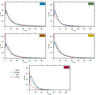
Fig. 7.Contribution to total annual precipitation by rainfall events of different intensity in the 5 precip-tiation regions for AWAP, bias-corrected and non-corrected WRF outputs, and GHCN stations.

25

Fig. 7. Contribution to total annual precipitation by rainfall events of different intensity in the 5 preciptiation regions for AWAP, bias-corrected

and non-corrected WRF outputs, and GHCN stations.

events according to their intensity as well as their occurrence is crucial to evaluate the risks and characterise their possible impact. The probability distribution of precipitation events is examined for AWAP, the stations and the two model out-puts to assess the performance of the bias correction at daily timescale and evaluate the potential benefits of using stations to correct high-resolution climate simulations.

The contribution to total precipitation by events of dif-ferent intensity is used instead of the traditional probability distribution function (PDF). Unlike the PDF, this alternative view of the probability distribution makes it easier to eval-uate the relative importance of the errors through the entire rainfall spectrum and includes information relative to the bias in the number of rain days for each of this intensities, which makes it preferable to this particular study.

Figure 7 summarises the contribution from rainfall events of different intensity in the 5 regions. This figure comple-ments the information provided by the monthly climatolo-gies (Fig. 4) and emphasises the differences amongst regions. Also, the comparison between distributions from observa-tional data sets yields important differences in all regions, es-pecially for precipitation events below 10 mm day−1, which

are systematically overestimated by AWAP. As for more in-tense events, AWAP tends to underestimate their contribu-tion to total precipitacontribu-tion in most regions; although, in the northeast (region 3) there is a clear overestimation. These differences are related to the difference in the spatial scales the observational products represent and suggest that AWAP, and more generally the observation-based grids, are not suit-able to correct model outputs with finer resolution. Ma-raun (2013) found that the use of stations to correct coarser RCMs (25 km×25 km) tend to inflate the variability of the model. We have looked into the quantile–quantile distribu-tion, which is basically an alternative representation of the probability distribution, to determine whether this occurs in our higher resolution simulation and found no evidence of such an artificial inflation of the variability (Supplement).

In most regions, WRF produces too much light pre-cipitation (0–2 mm day−1_{), underestimates moderate events}

Unlike seasonal biases, the daily precipitation distribution is not corrected adequately with this method due to the nega-tive biases in the number of rain days and both the original and the corrected model outputs show a persistent negative deviation across the entire spectrum of events, except for the very light events that are also overestimated. In this region, the validity of the assumption of a wetter model is compro-mised and thus the method might produce inaccurate results. However, while the bias correction is not able to com-pletely remove the errors, particularly in regions 4 and 5, it succeeds in providing a much better representation of the events distribution compared to the stations, which is a good indicator of the method’s skills. To quantify this improve-ment, the similarity between different PDFs was measured using the skill score (SS) proposed in Perkins et al. (2007), which calculates the common area shared by two PDFs. The SS confirms that the bias correction significantly improves the rain events distribution in the model over the entire do-main. Ordered by regions, the non-corrected model outputs and the in situ observations share 80.3 %, 70.2 %, 74.0 %, 76.1 % and 54.5 % of their precipitation PDFs, whereas the bias correction increases these percentages to 97.1 %, 95.1 %, 96.7 %, 96.6 % and 94.0 %, respectively. The im-provement is generally observed over the entire spectrum of intensities, but it might also be partly explained by rainfall events in the range 0–0.1 mm day−1that were not captured in the observations and did exist in the model outputs.

In the station data set, the precipitation with the largest contribution occur in the range between 2–6 mm day−1, whereas rain events below 2 mm day−1make a smaller con-tribution. This characteristic of rainfall distribution usually goes unnoticed in RCMs and is not captured by gridded data sets either, but it is better reproduced in the bias-corrected model outputs. This is a feature of daily precipitation that could play an important role in the hydrological cycle and thus represents a noteworthy improvement.

5 Conclusions

Bias correction has traditionally relied on the assumption that models produce more rain days than the reference observa-tions, which are usually gridded data sets due to their spa-tial and temporal characteristics. However, climate simula-tions are currently being completed at spatial resolusimula-tions that make this assumption no longer valid. A histogram equalisa-tion method (Piani et al., 2010a) was adapted to be used with stations, which are not subjected to more frequent low inten-sity precipitation due to spatial averaging. Although the use of stations do not completely overcome the bias correction limitations in areas of very strong dry biases, it makes the wet-day condition more likely to be fulfilled and thus signifi-cantly lessens the problem of rain-day frequency disparities. The stations were aggregated to bypass the two major ob-stacles for their use in bias correction, the differences in the

model and stations spatial scales, and the completeness and sparseness of the time series.

The method has been proven to substantially reduce the seasonal biases of precipitation when compared to both grid-ded and station data sets, even in areas where the wet-day condition was not met. Gridded data sets are also appropriate to correct high-resolution model at seasonal or even monthly timescales, but it has been shown here that they are not ad-equate to correct daily features of precipitation anywhere in the domain. Indeed, the major contribution of this study is the efficient bias correction of the daily precipitation proba-bility distributions of very high-resolution models. A much better representation of the frequency of the rainfall events is achieved after bias correction for all regions, especially in those where rainfall is overestimated. In areas where bi-ases are markedly dry, the method provides an improvement but the results are not as good due to differences in the wet-day occurrence. In general, the relative importance of mod-erate event with respect to very light ones is also better re-produced, which could also have important implications for impact assessment studies. We acknowledge that the avail-ability of a high-quality observation network is required to apply this bias correction method, but the generation of reli-able gridded data sets also need such a network. In this study, we have addressed issues related to precipitation, which is one of the most problematic variables in terms of bias cor-rection, but the method is applicable to other variables using different fitting functions and thus reduce biases due to mis-representation of local features such as the orography.

Supplementary material related to this article is

available online at http://www.hydrol-earth-syst-sci.net/ 17/4379/2013/hess-17-4379-2013-supplement.pdf.

Acknowledgements. This work was made possible by funding from the NSW Environment Trust (RM08603), as well as the NSW Office of Environment and Heritage, and the Australian Research Council as part of the Future Fellowship FT110100576. This work was supported by an award under the Merit Allocation Scheme on the NCI National Facility at the ANU.

Edited by: B. Su

References

Argüeso, D., Hidalgo-Muñoz, J. M., Gámiz-Fortis, S. R., Esteban-Parra, M. J., Castro-Díez, Y., and Dudhia, J.: Evaluation of WRF parameterizations for climate studies over Southern Spain using a multi-step regionalization, J. Climate, 24, 5633–5651, 2011. Argüeso, D., Evans, J. P., Fita, L., and Bormann, K. J.:

Tempera-ture response to fuTempera-ture urbanization and climate change, Clim. Dynam., doi:10.1007/s00382-013-1789-6, in press, 2013. Berg, P., Feldmann, H., and Panitz, H. J.: Bias correction of high

D. Argüeso et al.: High-resolution RCM precipitation bias correction 4387

Bordoy, R. and Burlando, P.: Bias Correction of Regional Climate Model Simulations in a Region of Complex Orography, J. Appl. Meteorol. Clim., 52, 82–101, 2013.

Chen, C., Haerter, J. O., Hagemann, S., and Piani, C.: On the con-tribution of statistical bias correction to the uncertainty in the projected hydrological cycle, Geophys. Res. Lett., 38, L20403, doi:10.1029/2011GL049318, 2011.

Christensen, J. H., Boberg, F., Christensen, O. B., and Lucas-Picher, P.: On the need for bias correction of regional climate change projections of temperature and precipitation, Geophys. Res. Lett., 35, L20709, doi:10.1029/2008GL035694, 2008. Déqué, M., Rowell, D. P., Lüthi, D., Giorgi, F., Christensen, J. H.,

Rockel, B., Jacob, D., Kjellstrom, E., de Castro, M., and Hurk, B. V. D.: An intercomparison of regional climate simulations for Europe: assessing uncertainties in model projections, Climatic Change, 81, 53–70, 2007.

Di Luca, A., de Elia, R., and Laprise, R.: Potential for added value in precipitation simulated by high-resolution nested Regional Cli-mate Models and observations, Clim. Dynam., 38, 1229–1247, 2011.

Ehret, U., Zehe, E., Wulfmeyer, V., Warrach-Sagi, K., and Liebert, J.: HESS Opinions “Should we apply bias correction to global and regional climate model data?”, Hydrol. Earth Syst. Sci., 16, 3391–3404, doi:10.5194/hess-16-3391-2012, 2012.

Evans, J. P. and McCabe, M.: Regional climate simulation over Aus-tralia’s Murray-Darling basin: A multitemporal assessment, J. Geophys. Res., 115, D14114, doi:10.1029/2010JD013816, 2010. Evans, J. P. and McCabe, M. F.: Effect of model resolution on a re-gional climate model simulation over southeast Australia, Clim. Res., 56, 131–145, 2013.

Evans, J. P. and Westra, S.: Investigating the Mechanisms of Diurnal Rainfall Variability Using a Regional Climate Model, J. Climate, 25, 7232–7247, 2012.

Feser, F., Rockel, B., von Storch, H., Winterfeldt, J., and Zahn, M.: Regional Climate Models Add Value to Global Model Data: A Review and Selected Examples, B. Am. Meteorol. Soc., 92, 1181–1192, 2011.

Giorgi, F.: Regional climate modeling: Status and perspectives, J. Phys. IV, 139, 101–118, 2006.

Gutjahr, O. and Heinemann, G.: Comparing precipitation bias cor-rection methods for high-resolution regional climate simula-tions using COSMO-CLM, Theor. Appl. Climatol., online first, doi:10.1007/s00704-013-0834-z, 2013.

Gutowski Jr., W., Decker, S., Donavon, R., Pan, Z., Arritt, R., and Takle, E.: Temporal-spatial scales of observed and simulated pre-cipitation in central U.S. climate, J. Climate, 16, 3841–3847, 2003.

Haerter, J. O., Hagemann, S., Moseley, C., and Piani, C.: Cli-mate model bias correction and the role of timescales, Hy-drol. Earth Syst. Sci., 15, 1065–1079, doi:10.5194/hess-15-1065-2011, 2011.

Hay, L., Wilby, R., and Leavesley, G.: A comparison of delta change and downscaled GCM scenarios for three mountainous basins in the United States, J. Am. Water Resour. As., 36, 387–397, 2000. Haylock, M. R., Hofstra, N., Tank, A. M. G. K., Klok, E. J., Jones, P. D., and New, M.: A European daily high-resolution gridded data set of surface temperature and precipitation for 1950–2006, J. Geophys. Res.-Atmos., 113, 1–12, 2008.

Jones, D. A., Wang, W., and Fawcett, R.: High-quality spatial climate data-sets for Australia, Australian Meteorological and Oceanographic Journal, 58, 233–248, 2009.

King, A. D., Alexander, L. V., and Donat, M. G.: The efficacy of using gridded data to examine extreme rainfall characteristics: a case study for Australia, Int. J. Climatol., 33, 2376–2387, 2012. Lafon, T., Dadson, S., Buys, G., and Prudhomme, C.: Bias

correc-tion of daily precipitacorrec-tion simulated by a regional climate model: a comparison of methods, Int. J. Climatol., 33, 1367–1381, 2013. Lenderink, G., Buishand, A., and van Deursen, W.: Estimates of future discharges of the river Rhine using two scenario method-ologies: direct versus delta approach, Hydrol. Earth Syst. Sci., 11, 1145–1159, doi:10.5194/hess-11-1145-2007, 2007. Maraun, D.: Bias Correction, Quantile Mapping, and

Downscal-ing: Revisiting the Inflation Issue, J. Climate, 26, 2137–2143, doi:10.1175/JCLI-D-12-00821.1, 2013.

Maraun, D., Wetterhall, F., Ireson, A. M., Chandler, R. E., Kendon, E. J., Widmann, M., Brienen, S., Rust, H. W., Sauter, T., The-meßl, M., Venema, V. K. C., Chun, K. P., Goodess, C. M., Jones, R. G., Onof, C., Vrac, M., and Thiele-Eich, I.: Precipita-tion downscaling under climate change: Recent developments to bridge the gap between dynamical models and the end user, Rev. Geophys., 48, RG3003, doi:10.1029/2009RG000314, 2010. Menne, M. J., Durre, I., Vose, R. S., Gleason, B. E., and

Hous-ton, T. G.: An Overview of the Global Historical Climatology Network-Daily Database, J. Atmos. Ocean. Tech., 29, 897–910, 2012.

Perkins, S. E., Pitman, A. J., Holbrook, N. J., and McAneney, J.: Evaluation of the AR4 climate models’ simulated daily maxi-mum temperature, minimaxi-mum temperature, and precipitation over Australia using probability density functions, J. Climate, 20, 4356–4376, 2007.

Piani, C. and Haerter, J. O.: Two dimensional bias correction of tem-perature and precipitation copulas in climate models, Geophys. Res. Lett., 39, L20401, doi:10.1029/2012GL053839, 2012. Piani, C., Haerter, J., and Coppola, E.: Statistical bias correction

for daily precipitation in regional climate models over Europe, Theor. Appl. Climatol., 99, 187–192, 2010a.

Piani, C., Weedon, G. P., Best, M., Gomes, S. M., Viterbo, P., Hage-mann, S., and Haerter, J. O.: Statistical bias correction of global simulated daily precipitation and temperature for the application of hydrological models, J. Hydrol., 395, 199–215, 2010b. Portoghese, I., Bruno, E., Guyennon, N., and Iacobellis, V.:

Stochastic bias-correction of daily rainfall scenarios for hydro-logical applications, Nat. Hazards Earth Syst. Sci., 11, 2497– 2509, doi:10.5194/nhess-11-2497-2011, 2011.

Rojas, R., Feyen, L., Dosio, A., and Bavera, D.: Improving pan-European hydrological simulation of extreme events through sta-tistical bias correction of RCM-driven climate simulations, Hy-drol. Earth Syst. Sci., 15, 2599–2620, doi:10.5194/hess-15-2599-2011, 2011.

Schmidli, J., Frei, C., and Vidale, P. L.: Downscaling from GCM precipitation: a benchmark for dynamical and statistical down-scaling methods, Int. J. Climatol., 26, 679–689, 2006.

Skamarock, W. C., Klemp, J. B., Dudhia, J., Gill, D. O., barker, D. M., Duda, M. G., Huang, X.-Y., Wang, W., and Powers, J. G.: A Description of the Advanced Research WRF Version 3, NCAR/TN-475+STR NCAR TECHNICAL NOTE, p. 125, 2009.

Terink, W., Hurkmans, R. T. W. L., Torfs, P. J. J. F., and Uijlenhoet, R.: Evaluation of a bias correction method applied to downscaled precipitation and temperature reanalysis data for the Rhine basin, Hydrol. Earth Syst. Sci., 14, 687–703, doi:10.5194/hess-14-687-2010, 2010.

Teutschbein, C. and Seibert, J.: Bias correction of regional climate model simulations for hydrological climate-change impact stud-ies: Review and evaluation of different methods, J. Hydrol., 456-457, 12–29, 2012.

Themeßl, M. J., Gobiet, A., and Leuprecht, A.: Empirical-statistical downscaling and error correction of daily precipitation from re-gional climate models, Int. J. Climatol., 31, 1530–1544, 2011. Themeßl, M. J., Gobiet, A., and Heinrich, G.: Empirical-statistical

downscaling and error correction of regional climate models and its impact on the climate change signal, Climatic Change, 112, 449–468, 2012.

Thompson, G., Field, P. R., Hall, W. D., and Rasmussen, R. M.: A new bulk microphysical parameterization for WRF (& MM5), Proc. Seventh Weather Research and Forecasting Model Work-shop, 1–11, 2006.