Very short term load forecasting of peak load time using Fuzzy type 2 and big bang big crunch (BBBC) algorithm

VERY SHORT-TERM LOAD FORECASTING OF PEAK LOAD TIME

USING FUZZY TYPE-2 AND BIG BANG BIG CRUNCH (BBBC)

ALGORITHM

Jamaaluddin Jamaaluddin

, Imam Robandi

, Izza Anshory

and Ahmad Fudholi

1

Program Studi Teknik Elektro, Universitas Muhammadiyah Sidoarjo, Jl. Raya Gelam No. 250, Candi, Jawa Timur, Indonesia

2

Departemen Teknik Elektro Institut Teknologi Sepuluh Nopember (ITS), Surabaya, Jawa Timur, Indonesia

3

Solar Energy Research Institute, Universiti Kebangsaan Malaysia, Bangi Selangor, Malaysia E-Mail: [email protected]

ABSTRACT

Very short-term energy forecasting is done on a day before the day of operation. Forecasting of short-term load is done every 30 minutes of forecasting hours. Very term load forecasting is carried out continuing forecasting short-term load with daily intervals, load on a given day or weekly load to be more detailed with very short-short-term load forecasting. This weight forecasting is done to improve operational effectiveness and efficiency. Forecasting short-term loads have been done using artificial intelligence, nowadays artificial intelligence is attempted to predict a very short term load. In this study, investigated the use of the Fuzzy type-2 (FT-2) and big bang big crunch (BBBC) algorithm for the very short-term load forecasting. Results shows that with the use of FT-2-BBBC, it will get a small error because it uses low computation cost and high convergent speed. In addition, FT-2 also optimizes the foot of uncertainty of the Fuzzy type-1. The results are in the use of FT-2-BBBC hence the very short term load forecasting error value of 0.7278%. This suggests that FT-2-BBBC can be used to perform electrical load forecasting and other forecasting.

Keywords: energy, electrical, power, load.

INTRODUCTION

The community needs of electrical energy is still very much. Electrical energy needs can be met using fossil fuel plants or using renewable energy. The use of fossil fuels for electrical energy generation is carried out using coal, solar and gas. The use of renewable energy is using solar energy and wind energy. There is a use of other sources for electric energy generation namely water, nuclear and other [1-4].

Utilization of electrical energy should be set as well. This setting starts from generation planning and load sharing, operation, setup and other matters [5]. Planning is done on the load side for generation planning. This plan is also known as forecasting. The electrical load forecasting is divided into three, i.e. long-term load forecasting, short-term load forecasting and extremely short-short-term load forecasting [6, 7].

This weight forecasting is necessary for consideration for the problem of consideration of efficiency and effectiveness of power generation and transmission of electricity loads. Arrangement of maintenance plans, labor arrangement and the arrangement of source supply of generation materials. It is related to economic problems [8].

year following the planning of the plant that will perform maintenance and repairs. This short-term load forecasting is done by conducting a daily peak load analyzer for one year. Meanwhile, for the very short period of electrical load forecasting is to plan the electricity load the next day. This very short-term electrical load forecasting is required to conduct detailed planning to adjust the current needs of electrical loads. This very short-term electrical load forecasting is done for the next day with a forecasting time interval of every 30 minutes [9, 10].

A very short period of electrical burden forecasting researchers who previously use artificial neural network (ANN) have a value (MAPE) between 0.89% - 1.25% [11]. Whereas when using based on autoregressive integrated moving average model (ARIMA) and intelligent systems have MAPE value if using ARIMA between 2.62%-5.27%, if using adaptive neuro-Fuzzy inference system (ANFIS) amounting to 10.21%-18.45% [12]. In the next development, there is a very short-term electrical load forecasting with the use of nonlinear autoregressive model with exogenous input (NARX-neural network), using this method in the get results MAPE between 0.5189% - 0.7973% [13].

the load spread across Java, Madura Island and Bali Island [17, 18]. This system is routinely done by using short-time load forecasting and very short time electrical load forecasting. This research is expected to provide better forecasting results than what has been previously done in Java Bali electricity system.

Historical loading data on the same day in the same month for the past 4 years is used to forecast a very short time electrical load forecasting. For the purposes of analysis, the examples out of peak load times are used at 13.00 - 15.30 (Western Indonesian Time) on the 4th Friday of the forecast day in October concerning the previous Friday loading, the 3rd Friday, 2nd Friday and 1st Friday in October.

The researcher tried to optimize the very short time load forecasting using Fuzzy type 2 interval - Fuzzy inference system hybridized with the BBBC algorithm, in

the expectation of getting a smaller error value [19, 20]. So that it can be applied to forecasting very short - time daily expenses.

MATERIAL AND METHOD

The stages of this research consist of pre-processing, processing and post-processing. The stages of the research will be explained as follows [21, 22].

Pre processing

The pre-processing stage is the preparation of daily load data every 30 minutes for 24 hours in a day, on the working day represented by Friday by classifying the out of peak load time which is at 13.00-15.30 to find the actual variation load difference, as the block diagram in Figure-1.

Figure-1. Pre processing stage. Processing

In processing, the VLD value obtained from the above calculation will be entered into the FT-2, at the

membership function with the following steps as Figure-2. The following input variables (X, Y) and output variables (Z) consist of 11 Fuzzy sets as shown in Figure-3.

After that, VLD (Variation Load Difference at Time) can be calculated at the predicted time.

𝑉𝐿𝐷(𝑖)= 𝐿𝐷(𝑖)− 𝑇𝐿𝐷(𝑖) ...(3)

𝑇𝐿𝐷(𝑖)= 𝐿𝐷(𝑖−1)₂− 𝐿𝐷(𝑖−2) … (2)

After that, the TLD (i) (The typical Time Load Difference) is

calculated by calculating the average load of LD(i) at each time

predicted by the same time last year and before.

𝐿𝐷(𝑖) = 𝑆𝐷(𝑖)_𝑇𝐷− 𝑇𝐷(𝑖)

(𝑖) 𝑥 100 … . (1)

Calculating the Difference Load at the same time on the fourth Friday (Time predicted). These results can be obtained using the formula below:

SD(i) is the load at the predicted time.

Figure-2. Processing stage.

FOU was designed in the range of 50% uncertainty from the upper and lower limits of the Fuzzy type-1 membership function [23-25]. This study covers six antecedent and consequent FOU uncertainty candidates which are optimized using the BBBC algorithm namely probability 44%, 46%, 48%, 50%, 52%, and 54% with objectively defined functions as 50%.

Load identification is sought 𝑇𝐷(𝑖) on Friday before the fourth Friday when the load is analyzed.

𝑇𝐷

=

Time Difference is the average load at the same time as different Fridays, namely first Friday

After the above process, the next step is to find the error value of the VLDmax forecast, done in the

following ways:

Calculating the forecast value of load difference for the predicted time using Equation (5):

F’cast LDMAX(i) = F’cast VLDMAX(i) +TLDMAX(i) (5)

The next step is to calculate the error value, using Equation (6):

𝐸𝑟𝑟𝑜𝑟 (%) =𝑃𝑓𝑜𝑟𝑒𝑐𝑎𝑠𝑡_𝑃 − 𝑃𝑎𝑐𝑡𝑢𝑎𝑙

𝑎𝑐𝑡𝑢𝑎𝑙 × 100 (6)

Where:

Pforecast = Power predicted at a certain time (MW).

Pactual = Actual power at a certain time (MW).

RESULTS AND DISCUSSIONS

The next step is to group the load in peak load conditions at each time starting in 2013, 2014, 2015, 2016 and 2017, the results of the grouping can be seen in table 1. The LD values are calculated in 2013 as in Equation (1) and (2). The result can seen in Figure-4.

Furthermore, for the 2015 loading year, the TD value and LD were obtained. From the electricity load data obtained in the 2015 TLD calculation value, using the Equation as shown in Equation no. (3), the 2015 TDL value is the one-year LD average value and LD value two years earlier. Whereas to get the VLD value in 2015, it is obtained by calculation as shown in Equation (4) that is from the 2015 LD value reduced by the 2015 TLD value. The results of the analysis in 2015 can be seen in Figure-5.

Figure-4. Comparison between forecasting and actual using IT-2 FIS.

For the TLD value in 2016, obtained the average value of LD 2015 and LD 2014. Whereas to get the 2016 VLD value, obtained from the 2016 LD value minus the 2016 TLD value. For the year of load calculation, 2017 TD, LD, TLD and VLD can be seen as in Figure-5.

Figure-5. VLD at 2015, 2016 and 2017.

The TLD value in 2017, obtained from the average LD 2016 and LD 2015 values. Meanwhile, the VLD 2017 value, obtained from the 2017 LD value minus the 2017 TLD value. The VLD values for 2016 and 2017, the X value of the 2016 VLD value is obtained and the output (Z) of the year VLD value is forecast in 2017, while the Y value is taken from the VLD value in 2017 for the adjacent time [20]. The result can seen in Table-1. After getting the X, Y and Z values, the next step is to enter the values into the membership function group.

13:00 13:30 14:00 14:30 15:00 15:30

2013 0,75 0,83 (0,43) 0,58 0,62 0,21

2014 (0,09) 1,22 0,39 0,33 (0,50) (0,41) (1,00)

(0,50) 0,50 1,00 1,50

L

oad

D

iff

e

r

e

nce

13:00 13:30 14:00 14:30 15:00 15:30

2015 0,78 (0,53) 0,60 0,64 1,46 1,70

2016 0,60 (0,36) 0,10 0,38 1,01 1,01

2017 (0,53) (0,44) (1,57) (1,70) (2,00) (1,43) (3,00)

(2,00) (1,00) 1,00 2,00

Table-1. Calculation of determining the values of X, Y and Z.

VLD VLD

Time 2016 2017 X Y Z

13:00 0.6027 (0.5295) 0.6027 (1.4308) (0.5295)

13:30 (0.3606) (0.4432) (0.3606) (0.5295) (0.4432)

14:00 0.0953 (1.5724) 0.0953 (0.4432) (1.5724)

14:30 0.3826 (1.7022) 0.3826 (1.5724) (1.7022)

15:00 1.0095 (1.9952) 1.0095 (1.7022) (1.9952)

15:30 1.0052 (1.4308) 1.0052 (1.9952) (1.4308)

Table-2. Based rule input X forecasting 2017.

Time Value Membership Function (μ) Sets

X NVB NB NM NS NVS ZE PVS PS PM PB PVB X

(5) (4) (3) (2) (1) - 1 2 3 4 5

13:00 0.6027 0.3973 0.6027 PVS

13:30 (0.3606) 0.3606 0.6394 ZE

14:00 0.0953 0.9047 0.0953 ZE

14:30 0.3826 0.6174 0.3826 PVS

15:00 1.0095 0.9905 0.0095 PVS

15:30 1.0052 0.9948 0.0052 PVS

Table-2 shows that the value of X at 13.00 is 0.6027 having a positive very small (PVS) membership degree of 0.6027, while the degree of membership value of zero (ZE) is 0.3973. Once the island for another X value is treated the same as the above calculation. That calculation is the same for the Y and Z.

From the data in Table 3, it is obtained the basic rules that are used to make the program in matlab, the rules are still in alphabetical form and will be changed to a number in order as in the order of the membership function above. The data can be seen in Table-4.

With the conversion as in Table-4, the matlab programming process can be done. Processing on matlab will generate value for VLD forecasting for 2017. After the process is done using matlab and found VLD forecasting in 2017 with the results as in Table-5. It shows very short term load forecasting in 2017 (out of peak load) fourth Friday October using IT-2 - BBBC.

Table-3. Conversion of 2017 basic forecasting rules. No of Antecendent Consequen

rules X Y Z

1 PVS NVS NVS

2 ZE NVS ZE

3 ZE ZE NS

4 PVS NS NS

5 PVS NS NS

6 PVS NS NVS

Table-4. Conversion of 2017 basic forecasting rules for the matlab software code.

No of Antecendent Consequen

rules X Y Z

Table-5. Results of VLD calculation in 2017 using FT-2 BBBC (output matlab).

Actual Forecasting Error

VLD VLD VLD

-0.5295 -1.0018 0.4723

-0.4432 -0.825 0.3819

-1.5724 -1.1637 0.4087 -1.7022 -1.1374 0.5648 -1.9952 -1.4083 0.5869 -1.4308 -1.3979 0.0329

Table-6 shows the comparison of the value of power (P) forecasting results with the actual power (P)

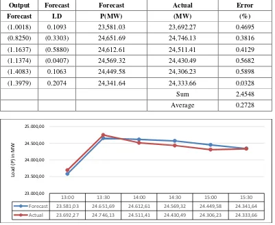
value. Therefore, the error value can be calculated. In Table 6, it can be seen that the average error forecasting value using FT-2 - BBBC is as shown in Table-6. Table 6 and Figure-6, shows the comparison of the value of power (P) forecasting results with the actual power (P) value. Therefore, the error value can be calculated. Indicates the average error forecasting value using FT-2-BBBC is 0.2728%. Figure-6 shows a comparison between the electricity load forecasting and the actual electricity load at the time of the peak load every 30 minutes starting at 13.00 until 15:30.

Figure-7 shows that FT-2 which is optimized with BBBC in the process of forecasting a very short term load produces a small error value. So that this can be used for the electric load control agency in forecasting very short term loads on the 1 day before the operational day to get the optimal operation of the power plant.

Table-6. Comparative value of 2017 forecasting and actual load expenses using FT-2-BBBC.

Output Forecast Forecast Actual Error

Forecast LD P(MW) (MW) (%)

(1.0018) 0.1093 23,581.03 23,692.27 0.4695 (0.8250) (0.3303) 24,651.69 24,746.13 0.3816 (1.1637) (0.5880) 24,612.61 24,511.41 0.4129 (1.1374) (0.0407) 24,569.32 24,430.49 0.5682 (1.4083) 0.1063 24,449.58 24,306.23 0.5898 (1.3979) 0.2074 24,341.64 24,333.66 0.0328

Sum 2.4548

Average 0.2728

Figure-6. Comparison between forecasting and actual using FT-2 BBBC. 13:00 13:30 14:00 14:30 15:00 15:30 Forecast 23.581,03 24.651,69 24.612,61 24.569,32 24.449,58 24.341,64 Actual 23.692,27 24.746,13 24.511,41 24.430,49 24.306,23 24.333,66

23.000,00 23.500,00 24.000,00 24.500,00 25.000,00

Lo

ad

(

P

) i

n

M

Figure-7. Error forecasting 2017 using FT-2-BBBC.

CONCLUSIONS

The findings of the research are as follows: a) Optimization of the footprint of uncertainty (FOU) of

Fuzzy type-2 using BBBC algorithm for forecasting very short time loads at peak load shows an average small error (0.2728%).

b) The use of BBBC algorithm in FT-2 optimization can be used to optimize the forecasting of other things.

ACKNOWLEDGEMENTS

The authors would like to thanks the Universitas Muhammadiyah Sidoarjo for funding this research. REFERENCES

[1] A. Supriyadi, J. Jamaaluddin, T. Elektro, and U. Muhammadiyah. 2018. Analisa Efisiensi Penjejak Sinar Matahari Dengan Menggunakan. Jeee-U. 2(APRIL): 8-15.

[2] S. Younes, R. Claywell and T. Muneer. 2005. Quality control of solar radiation data: Present status and proposed new approaches. in Energy. 30(9)SPEC. ISS., 1533-1549.

[3] A. Supriyadi, J. Jamaaluddin, T. Elektro, and U. Muhammadiyah. 2018. ANALISA EFISIENSI PENJEJAK SINAR MATAHARI DENGAN MENGGUNAKAN. JEEE-U.

[4] M. Yahya, A. Fudholi and K. Sopian. 2017. Energy and exergy analyses of solar-assisted fluidized bed

[6] L. Suganthi, S. Iniyan and A. A. Samuel. 2015. Applications of fuzzy logic in renewable energy systems - A review. Renew. Sustain. Energy Rev. 48: 585-607.

[7] M. Rumbayan, A. Abudureyimu and K. Nagasaka. 2012. Mapping of solar energy potential in Indonesia using artificial neural network and geographical information system. Renew. Sustain. Energy Rev. 16(3): 1437-1449.

[8] J. Jamaaluddin, D. Hadidjaja, I. Sulistiyowati, E. A. Suprayitno, I. Anshory and S. Syahrorini. 2018. Very short term load forecasting peak load time using fuzzy logic. in IOP Conference Series: Materials Science and Engineering.

[9] A. Setiawan, I. Koprinska, and V. G. Agelidis. 2009. Very short-term electricity load demand forecasting using support vector regression. 2009 Int. Jt. Conf. Neural Networks. pp. 2888–2894.

[10]S. A. Soliman and A. M. Al-Kandari, 8 Dynamic Electric Load Forecasting. 2010.

[11]W. Charytoniuk and M.-S. Chen. 2000. Very Short-Term Load Forecasting Using Artificial Neural Networks. IEEE Trans. Power Syst. 15(1): 263.

[12]L. C. Moreira de Andrade and I. Nunes da Silva. 2009. Very Short-Term Load Forecasting Based on ARIMA Model and Intelligent Systems. 2009 15th 13:00 13:30 14:00 14:30 15:00 15:30

Datenreihen1 0,4695 0,3816 0,4129 0,5682 0,5898 0,0328

0,1000 0,2000 0,3000 0,4000 0,5000 0,6000 0,7000

E

rr

o

[14]P. P. (PERSERO) P. J. B. - B. O. Sistem. 2014. EVALUASI OPERASI SISTEM TENAGA LISTRIK JAWA BALI 2014, 1st ed. Jakarta.

[15]P. P. (PERSERO) P. J. B. - B. O. Sistem. 2013. EVALUASI OPERASI SISTEM TENAGA LISTRIK JAWA BALI 2013, 1st ed. Jakarta: PT PLN (PERSERO) P3B Jawa Bali - Bidang Operasi Sistem.

[16]International Energy Agency. 2015. World Energy Outlook 2015. Executive Summary. Int. Energy Agency books online.

[17]P. P. (PERSERO) P. - B. Perencanaan, EVALUASI OPERASI SISTEM TENAGA LISTRIK JAWA BALI 2015, 01 ed. Jakarta: PT PLN (PERSERO) P2B – Bidang Perencanaan, 2015.

[18]Sekretariat Perusahaan PT. PLN. 2015. Statistik PLN 2014. no. 02701, p. iv.

[19]O. K. Erol and I. Eksin. 2006. A new optimization method: Big Bang-Big Crunch. Adv. Eng. Softw. 37(2): 106-111.

[20]T. Kumbasar and H. Hagras. 2013. A big bang-big crunch optimization based approach for interval type-2 fuzzy PID controller design. IEEE Int. Conf. Fuzzy Syst.

[21]A. Ramadhani, I. Robandi, J. T. Elektro and F. T. Industri. 2015. Optimisasi Peramalan Beban Jangka Pendek untuk Hari Libur Nasional Menggunakan Interval Type-2 Fuzzy Inference System-Big Bang-Big Crunch Algorithm (Studi Kasus : Sistem Kelistrikan Kalimantan Selatan dan Tengah). pp. 1-8.

[22]Jamaaluddin, I. Robandi and I. Anshory. 2019. A very short-term load forecasting in time of peak loads using interval type-2 fuzzy inference system: A case study on java bali electrical system. J. Eng. Sci. Technol. 14(1): 464-478.

[23]M. Biglarbegian, W. W. Melek and J. M. Mendel. 2010. On the stability of interval type-2 tsk fuzzy logic control systems. IEEE Trans. Syst. Man, Cybern. Part B Cybern. 40(3): 798-818.

[24]Jamaaluddin; Imam Robandi. 2016. Short Term Load Forecasting of Eid Al Fitr Holiday By Using Interval Type - 2 Fuzzy Inference System (Case Study : Electrical System of Java Bali in Indonesia). in 2016 IEEE Region 10, TENSYMP. 0(x): 237-242.