Copula based statistical refinement of precipitation in RCM simulations over complex terrain

www.hydrol-earth-syst-sci.net/15/2401/2011/ doi:10.5194/hess-15-2401-2011

© Author(s) 2011. CC Attribution 3.0 License.

Earth System

Sciences

Copula-based statistical refinement of precipitation in RCM

simulations over complex terrain

P. Laux1, S. Vogl2, W. Qiu1, H. R. Knoche1, and H. Kunstmann1,2

1_{Karlsruhe Institute of Technology (KIT), Institute for Meteorology and Climate Research (IMK-IFU),}

Kreuzeckbahnstrasse 19, 82467 Garmisch-Partenkirchen, Germany

2_{University of Augsburg, Institute for Geography, Regional Climate and Hydrology, 86135 Augsburg, Germany}

Received: 17 March 2011 – Published in Hydrol. Earth Syst. Sci. Discuss.: 29 March 2011 Revised: 27 June 2011 – Accepted: 27 July 2011 – Published: 29 July 2011

Abstract. This paper presents a new Copula-based method for further downscaling regional climate simulations. It is developed, applied and evaluated for selected stations in the alpine region of Germany. Apart from the common way to use Copulas to model the extreme values, a strategy is pro-posed which allows to model continuous time series. As the concept of Copulas requires independent and identically distributed (iid) random variables, meteorological fields are transformed using an ARMA-GARCH time series model. In this paper, we focus on the positive pairs of observed and modelled (RCM) precipitation. According to the empirical copulas, significant upper and lower tail dependence between observed and modelled precipitation can be observed. These dependence structures are further conditioned on the prevail-ing large-scale weather situation. Based on the derived theo-retical Copula models, stochastic rainfall simulations are per-formed, finally allowing for bias corrected and locally refined RCM simulations.

1 Introduction

GCMs and RCMs are a central prerequisite for conducting climate change impact studies that require time series of cli-matic variables. The projections of future climate usually fol-low the so-called delta-change approach, considering the dif-ferences between present and future climate. If time series of RCMs are used directly as input for external impact models such as hydrological or agricultural models with nonlinear responses to the climate signal, the delta-change approach may fail (e.g., Graham et al., 2007; Sennikovs and Bethers, 2009). One reason is the spatial resolution which does not

Correspondence to: P. Laux

([email protected])

allow for local scale climate differences, particularly in com-plex terrain. Usually there exist tremendous biases between modelled and observed climate statistics (e.g. Schmidli et al., 2007; Smiatek et al., 2009). Therefore, further statistical re-finement and bias correction methods are required to obtain reliable meteorological information at local scale (Wilby and Wigley, 1997). Precipitation is one of the most important variables for climate change impact studies (Schmidli et al., 2006). At the same time it is the most difficult to model.

Statistical downscaling and bias correction methods can be divided into (i) direct point-wise techniques which relate spe-cific (mostly adjacent) RCM grid cells to a station of interest such as mean value adaptation (e.g. Kunstmann et al., 2004; Jung and Kunstmann, 2007), quantile mapping/histogram equalization methods (e.g. Leung et al., 1999; Wood et al., 2002; Themeßl et al., 2010; Senatore et al., 2011) or local in-tensity scaling (e.g. Schmidli et al., 2006; Yang et al., 2010), and (ii) indirect methods which relate meteorological fields to the station such as the analogue method (e.g. Bliefernicht and B´ardossy, 2007), weather or circulation pattern classifi-cation techniques (e.g. B´ardossy et al., 2002), or empirical orthogonal functions (e.g. von Storch and Zwiers, 1999).

Fig. 1. Terrain elevation (left), and bias of mean annual total precipitation for the RCM (MM5) with respect to the DWD reference data set [%] (Kotlarski et al., 2005) (right).

especially during the summer season with prevailing convec-tive rainfall processes (e.g. Schmidli et al., 2007). Potential reasons for this are e.g. (i) the variability of observed rainfall within one corresponding modelled grid cell could be very high; rain gauges in the near surrounding can measure large differences in rainfall amounts; (ii) difficulties to capture the location of convective rainfall events by the climate models; this is mostly due to coarse resolution of the land surface model (LSM) and the partly chaotic nature of convection, and (iii) wrong or inadequate model parameterizations for convection.

The dependence structures of multivariate distributions can be modelled using classical distributions such as a mul-tivariate normal. However, it is obvious that a Gaussian ap-proach can not adequately reproduce the dependence struc-tures whenever large asymmetries are existing. In these cases, a Copula approach is supposed to be superior because Copula functions can be adapted flexibly to the data. In ad-dition to that, there already exists a large pool of theoretical models which are capable to describe individual characteris-tics of the data.

Copulas are additionally advantageous as they allow for describing the dependence structure independently from the marginal distributions (e.g. Genest and Favre, 2007; Dupois, 2007), and thus, using different marginal distributions at the same time without any transformations.

There is an increase in applications of Copulas in hy-drometeorology over the past years. Copula-based models have been introduced for multivariate frequency analysis, risk assessment, geostatistical interpolation and multivari-ate extreme value analyses (e.g. De Michele and Salvadori, 2003; B´ardossy, 2006; Genest and Favre, 2007; Renard and Lang, 2007; Sch¨olzel and Friederichs, 2008; B´ardossy and Li, 2008; Zhang and Singh, 2008).

For rainfall modelling, De Michele and Salvadori (2003) used Copulas to model intensity-duration of rainfall events. Favre et al. (2004) utilized Copulas for multivariate hydro-logical frequency analysis. Zhang and Singh (2008) carried out a bivariate rainfall frequency analysis using Archimedean Copulas. Renard and Lang (2007) investigated the usefulness of the Gaussian Copula in extreme value analysis. Kuhn et al. (2007) employed Copulas to describe spatial and tempo-ral dependence of weekly precipitation extremes. Serinaldi (2008) studied the dependence of rain gauge data using the non-parametric Kendall’s rank correlation and the upper tail dependence coefficient (TDC). Based on the properties of the Kendall correlation and TDC, a Copula-based mixed model for modelling the dependence structure and marginals is sug-gested. Recently, Copula-based models for estimating er-ror fields of radar information are developed (Villarini et al., 2008; AghaKouchak et al., 2010a,b). The intermittent nature of daily and sub-daily rainfall time series (zero-inflated data) can be modelled by mixed distributions, which are distribu-tions with a continuous part describing data larger than zero and a discrete part accounting for probabilities to observe zero values (Serinaldi, 2009). While the univariate form of such distributions was studied by many authors, the bi- or multivariate case received less attention (Serinaldi, 2009). Serinaldi (2009a) developed a copula-based rainfall model which is able to jointly account for discrete and continuous nature of observed daily rainfall, and can be used for simulat-ing rainfall at multiple sites. Similarly, B´ardossy and Pegram (2009) present a method to model the spatial interdependence structure of the rainfall amounts together with the rainfall oc-currences.

Conventional rainfall models operate under the assump-tion of either constant variance or season-dependent vari-ances using an AutoRegressive Moving Average (ARMA)

Fig. 2. Alpine region showing the location of observation stations used in this paper: 1 Garmisch-Partenkirchen, 2 Grainau, 3 Grainau (Eibsee), 4 Bad Reichenhall, 5 Schneizlreuth-Unterjettenberg, 6 Schneizlreuth-Ristfeucht, 7 Schneizlreuth-Weissbach, 8 Anger-Oberh ¨ogl, 9 Bischofswiesen-Winkl, 10 Inzell, 11 Anger-Stoissberg, 12 Rottach-Egern, 13 Kreuth, and 14 Schwarzkopfh ¨utte.

36

Fig. 2. Alpine region showing the location of observation stations used in this paper: 1 – Garmisch-Partenkirchen, 2 – Grainau, 3 – Grainau (Eibsee), 4 – Bad Reichenhall, 5 – Schneizlreuth-Unterjettenberg, 6 – Schneizlreuth-Ristfeucht, 7 – Schneizlreuth-Weissbach, 8 – Anger-Oberh¨ogl, 9 – Bischofswiesen-Winkl, 10 – Inzell, 11 – Anger-Stoissberg, 12 – Rottach-Egern, 13 – Kreuth, and 14 – Schwarzkopfh¨utte.

model. However, it could be shown that daily rainfall data are affected by non-linear characteristics of the variance often referred to as variance clustering or volatility, in which large changes tend to follow large changes, and small changes tend to follow small changes. This nonlinear phenomenon of the variance behaviour can be found e.g. in monthly and daily streamflow data (Wang et al., 2005), but also in meteorologi-cal time series such as temperature (Romilly, 2005). It is an-alyzed in this paper if volatility in daily precipitation series can be modelled using Generalized AutoRegressive Condi-tional Heteroskedasticity (GARCH) models.

This paper addresses the questions of (i) how to model the temporal characteristics, i.e. serial dependence and time varying variance (volatility) of daily rainfall series, and (ii) how to describe the complex joint dependence struc-ture of measured daily rainfall series and corresponding sim-ulated rainfall series obtained from a RCM model. The method of choice in this paper is the bivariate Copula. The dependence structure is investigated for each observation sta-tion separately.

The innovation of this paper mainly is:

– Application of an ARMA-GARCH algorithm to ana-lyze daily precipitation time series for seasonal vari-ation and volatility, and to generate independent and identically distributed (hereinafter iid) residuals for the Copula approach.

– Description and modelling of the joint dependence structure between RCM modelled and observed precipitation, accounting for the prevailing flow situa-tions caused by large-scale circulation patterns.

2 Regional climate model simulations and observed data

Regional climate simulations used in this study are based on the Penn State/NCAR Mesoscale Model (MM5) and ECMWF/ERA15 reanalysis data for 1979–1993 at 19.2 km spatial resolution. The climate simulations have been carried out within the framework of the QUIRCS-DEKLIM project (Kotlarski et al., 2005). A comparison of the MM5 simu-lations with gridded observation data for Germany obtained from the German weather service (DWD) reveal that rain-fall is overestimated by MM5 for the eastern part of Ger-many, and strongly underestimated for the Rhine valley and the alpine region of Germany (Fig. 1, right). The underes-timation in the alpine region is possibly due to the complex terrain with strong gradients of altitude (Fig. 1, left).

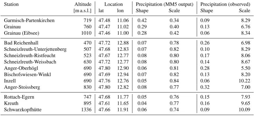
In order to statistically refine and correct precipitation ob-tained by RCM (MM5) climate simulations, daily rainfall data of 132 observation stations within the alpine region of Germany are retrieved from the webwerdis data portal of the DWD. Our study focusses on the alpine subregion round Garmisch-Partenkirchen. For the analysis of the dependence structure between modelled and observed precipitation, a subset of 14 observation stations with large altitudinal dif-ferences is selected (see Fig. 2 and Table 1). These stations correspond to three different grid cells of the RCM output where the model bias is comparatively large.

3 Modelling the dependence structure between modelled and observed rainfall

Fig. 3. Concept of the bias correction followed in this paper.

37

Fig. 3. Concept of the bias correction followed in this paper.

rainfall, and to finally generate random samples of locally re-fined and bias corrected pseudo-observations, requires mul-tiple steps (Fig. 3) that can be comprised as follows:

1. A suitable ARMA-GARCH model is fitted to the modelled and observed rainfall series (positive values only) to capture the seasonal variation of variance (see Sect. 3.1.1) of both RCM simulated and station ob-served precipitation.

2. The marginals are fitted to semi-parametric Generalized Pareto Distributions (GPD) for an improved representa-tion of the tails (see Sect. 3.1.2).

3. The bivariate empirical Copula (bivariate probability density plot), which is independent from their corre-sponding marginal distributions, is derived from the residuals of the ARMA-GARCH model.

4. A theoretical Copula model is estimated using the iid residuals obtained from the ARMA-GARCH model (see Sect. 3.2.2).

5. Stochastic simulations are performed using the condi-tional CDF of the theoretical Copula (see Sect. 3.2.3) and the univariate distributions of the original data (pos-itive pairs only).

6. Stochastic simulations are performed using conditional CDFs of the theoretical Copula of different large-scale weather patterns (see Sect. 3.3).

3.1 Modelling the marginals

Modelling the joint dependence structure requires that the marginals are iid. Most climatological time series, however exhibit some degree of autocorrelation and heteroskedastic-ity. In the sequel the ARMA-GARCH composite model to generate iid variables is introduced, followed by the descrip-tion of how to fit a GPD to the marginals, and to derive a joint distribution function (Copula) to model the dependence between modelled and observed rainfall time series.

3.1.1 ARMA-GARCH filter

This section describes briefly the theory of the ARMA-GARCH composite model and how it is used to simulate the univariate time series in the presence of conditional mean as well as conditional time-varying variance on daily time scale, i.e. heteroskedasticity or volatility, to produce iid resid-uals. An ARMA model is used to compensate for auto-correlation, and a GARCH model to compensate for the heteroskedasticity.

The term conditional in GARCH – Generalized Autore-gressive Conditional Heteroskedasticity – implies explicitely the dependence on a past sequence of observations, and

au-toregressive describes a feedback mechanism that

incorpo-rates past observations into the present. GARCH is a time series modelling technique that includes past variances for predicting present or future variances.

A univariate model of an observed time seriesyt can be

written as

yt =E (yt|t−1)+εt. (1)

In this equation, the termE (·|·)denotes the conditional expectation operator,t−1the information set at timet−1,

andεt the innovations at timet. Bollerslev (1986)

devel-oped GARCH as a generalization of the ARCH volatility modelling technique (Engle, 1982). The distribution of the residuals, conditional on the timet, is given by

Vart−1(yt) = Et−1

ε2_t = σ_t2 (2)

where

σ_t2 = κ +

P X

i=1

Gi σt2−i + Q X

j=1

Aj ε2t−j (3)

whereκis a constant, andσ_t2is the prediction of the variance, given the past sequence of variance predictions, σ_t2_−i, and past realizations of the variance itself,ε2_t−j. WhenP= 0, the GARCH(0,Q) model becomes the original ARCH(Q) model introduced by Engle (1982). This equation mimics the vari-ance clustering of the variable (i.e. precipitation and temper-ature). The lag lengthsP andQand the coefficientsGi and

Ajdetermine the degree of persistence.

Table 1. Station informations corresponding to 3 chosen MM5 grid cells, shape (tail index), and scale parameters of the fitted Generalized Pareto Distribution (GPD) for positive pairs of modelled and observed precipitation respectively.

Station Altitude Location Precipitation (MM5 output) Precipitation (observed)

[m a.s.l.] lat lon Shape Scale Shape Scale

Garmisch-Partenkirchen 719 47.48 11.06 0.42 0.34 0.09 8.29

Grainau 760 47.47 11.02 0.29 0.40 0.13 6.76

Grainau (Eibsee) 1010 47.46 11.00 0.28 0.42 0.06 8.34

Bad Reichenhall 470 47.72 12.88 0.07 0.78 0.26 6.98

Schneizlreuth-Unterjettenberg 507 47.68 12.83 0.07 0.82 0.10 8.29

Schneizlreuth-Ristfeucht 523 47.67 12.77 0.08 0.80 0.17 8.06

Schneizlreuth-Weissbach 630 47.72 12.77 0.08 0.80 0.14 8.67

Anger-Oberh¨ogl 690 47.80 12.90 0.06 0.81 0.28 5.50

Bischofswiesen-Winkl 690 47.69 12.94 0.07 0.82 0.13 8.20

Inzell 690 47.76 12.76 0.05 0.84 0.06 10.22

Anger-Stoissberg 830 47.80 12.82 0.08 0.77 0.32 7.00

Rottach-Egern 747 47.68 11.77 0.05 0.76 0.15 7.93

Kreuth 895 47.61 11.65 0.04 0.77 0.16 9.65

Schwarzkopfh¨utte 1336 47.66 11.91 0.06 0.74 0.09 10.09

A common assumption is that the innovations are serially independent, however, GARCH(P,Q) innovations,{εt}, are

modelled as

εt = σtzt. (4)

σt is the conditional standard deviation given by the square

root of Eq. (3), andzt is the standardized iid random draw

from some specified probability distribution. Usually, a Gaussian distribution is assumed such thatε∼N (0, σ_t2). Re-flecting this, Eq. (4) illustrates that a GARCH innovations process{εt}simply rescales an iid process{zt}such that the

conditional standard deviation incorporates the serial depen-dence of Eq. (3).

3.1.2 Generalized pareto distribution

This subsection describes the fitting of semi-parametric cu-mulative distribution functions (CDFs). First, the empirical CDF of each parameter is estimated using a Gaussian kernel function (using a kernel width of 50 points) to eliminate the staircase pattern. This provides a reasonably good fit to the interior of the distribution of the residuals. This procedure, however, tends to perform poorly when applied to upper and lower tails.

The upper and lower tails therefore are fitted separately from the interior of the distribution. For this reason, the peaks over threshold (POT) method is applied: A threshold value of 0.1 is chosen, i.e. the upper and lower 10 % of the residuals are reserved for each tail. The extreme residuals (beyond the threshold) are fitted to a parametric GPD, which can be described as

y = f (x|k, σ, θ ) =

₁

σ 1+k

_{(x −θ )}

σ

−1−1_k

(5)

using a maximum likelihood approach. Given the ex-ceedances in each tail, the negative log-likelihood function is optimized to estimate the tail index/shape parameterkand the scale parameterσof the GPD. The composite GPD func-tion allows for interpolafunc-tion in the interior of the CDF but also for extrapolation in the lower and upper tails.

3.2 Copula based joint distribution functions of modelled and observed rainfall

Copulas are functions that link multivariate distribu-tion F (x1, ... xn) to their univariate marginals FXi(xi).

Sklar (1959) proved that every multivariate distribution F (x1, ... xn)can be expressed in terms of a CopulaC and

its marginalsFXi(xi):

F (x1, ... xn) = C FX1 (x1), ..., FXn (xn)

(6)

C : [0,1]n → [0,1]. (7)

Copulas allow to merge the dependence structure and the marginal distributions to form a joint multivariate distribu-tion. The Copula function is unique when the marginals are continuous functions. As the Copula is a reflection of the dependency structure itself, its construction is reduced to the study of the relationship between the variables, giving free-dom for the choice of the univariate marginal distributions. Further information about Copulas can be found e.g. in Joe (1997); Frees and Valdez (1998); Nelsen (1999); Salvadori et al. (2007).

modelled by the multivariate normal distribution. The com-plex multivariate dependence structure is analyzed between RCM modelled precipitation (MM5 output) and station ob-served precipitation.

For dry days only the single marginal distributions ex-ist (Yang, 2008) but no (unique) joint dex-istribution function. Consequently, it is not possible to estimate a Copula model for dry days without further transformations such as nor-mal score. For sake of simplicity, we focus our work on the positive pairs (RCM precipitation>0, observed precip-itation>0).

3.2.1 Empirical Copula

The dependence structure of daily measured precipitation and simulated precipitation is studied. Since the underlying (theoretical) Copula is not known in advance, it is necessary to analyze the empirical Copula, which is purely based on the data (Deheuvels, 1979). The ranks of the residuals of mod-elled and observed rainfall from day 1 to dayn, obtained from the original data as well as the ARMA-GARCH time series model, are{r1(1), ..., r1(n)}and{r2(1), ..., r2(n)},

respectively. The empirical Copula is defined as: Cn(u,v) = 1/n

n X

t=1

1

r1(t )

n 6 u, r2(t )

n 6 v

(8) where u indicates the percentile of the modelled rainfall residuals,vindicates the percentile of the measured rainfall residuals and 1(...)is denoting the indicator function. 3.2.2 Copula goodness-of-fit test

A goodness-of-fit test for Copulas is applied comparing the empirical CopulaCn(Eq. 8) with the parametric estimate of a

theoretical Copula modelCθderived under the null

hypothe-sis. This is done for the residual series (Gr´egoire et al., 2008) of observed and modelled rainfall obtained by the ARMA-GARCH transformation. The test is based on the Cram´er-von Mises statistic (Genest and Favre, 2007):

Sn = n n X

t=1

{Cθ (ut, vt) −Cn (ut, vt)}2. (9)

As the definition of Sn involves the theoretical Copula

function, the distribution of this statistic depends on the un-known value ofθunder the null hypothesis thatCis from the classCθ (Gr´egoire et al., 2008). Therefore, the approximate

p-values for the test statistic are obtained using a parametric bootstrap (Genest and Remillard, 2008; Genest et al., 2009) as well as a fast multiplier approach (Kojadinovic and Yan, 2011a,b).

3.2.3 Relationship between Copula parameterθand rank-based concordance measures

There is a functional relationship between the classical de-pendence parameters such as Kendall’sτ and Spearman’sρ

namely ρ = 12

Z Z

[0,1]2

u v dCθ(u, v) −3 = 12 Z Z

[0,1]2

Cθ(u, v) du dv −3 (10)

and τ = 4

Z Z

[0,1]2

Cθ (u, v) dCθ (u, v)−1 (11)

or for Archimedean Copulas with generatorϕ τ = 1 +4

Z

[0,1]

ϕ(t )

ϕ0_{(t )}. (12)

For the Gumbel-Hougaard Copula with its generator ϕ(t )=(−ln(t ))θ it is found thatθ=₁₋1_τ, soθis a increasing function ofτ. According to this empirical link Kendall’sτ can be used as a rank-based estimator for the Copula param-eterθ. In turn, this link enables the interpretation of the Cop-ula parameter as a measure for the strength of dependence: higher Copula parameters reveal a stronger dependence. 3.2.4 Copula-based rainfall simulations

After the estimation of the Copula-based joint distribution – that isFX(x),FY(y)andCθ(u,v)are obtained – conditional

random samples from this distribution are generated through Monte Carlo simulations. We follow the procedure of Sal-vadori et al. (2007) for the conditional simulation using Cop-ulas. The simulation is based on conditional probabilities of the form:

P (V ≤ v|U = u) = ∂

∂u C (u, v); (13)

P (U ≤ u|V = v) = ∂

∂v C (u, v). (14)

For the Gumbel-Hougaard Copula e.g. it is: ∂

∂uC(u,v) =u

−1_e−(log(u)θ)+(log(v)θ)1/θ

(−log(u))−1+θ((−log(u)θ)+(−log(v))θ)−1+1/θ. (15) The concept for simulation of pseudo-observation from model data is as follows: a pair of variates(u, v)with Cop-ulaC(u, v)needs to be generated which finally can be trans-formed into(x, y), using the probability integral transforma-tion

U = FX(x) ⇔ X = F_X−1(U ) (16)

V = FY(y) ⇔ Y = F_Y−1(V ). (17)

The complete algorithm is divided into three steps: 1. Computationu=FX(x), wherex denotes one value of

the modelled rainfall andFX(x)is the marginal

distri-bution of the variateX.

2. Generation of random samples for the variatev∗from the conditional CDFCV|U(v|u)=cu(v)and calculation

ofv=c_u−1(v∗), wherec−_u1 denotes the generalized in-verse ofcu(Nelsen, 1999).

3. Calculation of the corresponding y-values using the probability integral transformationF_Y−1(v)=y. The final result fory is a sample of pseudo-observations which lies in the original data space and can be compared with the observed data series.

3.3 Usability of weather patterns for conditional simulations

Especially for complex terrain, it is assumed that the direc-tion of advecdirec-tion is of crucial importance for the observed precipitation amounts. The combinations of terrain exposi-tion and advecexposi-tion direcexposi-tion leads to luv and lee side effects, i.e. the stations can lie in the rainshadow or can be exposed to intense rainfall. As independent from the RCM simulations, large-scale weather patterns are used to further improve the results of the bias correction. Besides the advection direc-tion, large scale information about cyclonality and tropo-spheric humidity is evaluated. The objective weather pattern classification method of the German Weather Service is used (Bissolli and Dittmann, 2001). The classification domain is Central Europe, and the meteorological criteria for the classi-fication are (i) the direction of advection of air masses, (ii) the cyclonality, and (iii) the humidity of the troposphere. This leads to numerical indices from which the weather types are derived (Bissolli and Dittmann, 2001). There exist 40 prede-fined types, which can be used. Due to the limited occurrence frequencies of single weather types, their usability for con-ditional simulations is restricted. However, the usage of the numerical indices provides the possibility to group the types to different classes.

For this study, the following grouping strategies are evaluated:

1. Grouping types due to the direction of the advection of

air masses at 700 hPa: the weather types (WTs) are

grouped into northeasterly, southeasterly, southwest-erly, and northwesterly flow.

2. Grouping types due to the cyclonality at 950 hPa and

500 hPa: this leads to four classes, namely anticyclonal

– anticyclonal (AA), anticyclonal – cyclonal (AC), cy-clonal – anticycy-clonal (CA), and cycy-clonal – cycy-clonal (CC).

3. Grouping types due to the humidity of the

tropo-sphere: this leads to the discrimination of dry (D) and

wet (W). Therefore, a humidity index is calculated as the weighted areal mean of the precipitable water inte-grated over the 950, 850, 700, 500, and 300 hPa levels.

For each group of weather types, a theoretical Copula model is estimated separately. For sake of simplicity, the Gumbel-Hougaard Copula model is used.

3.4 Performance of simulations

To quantitatively evaluate the performane of the stochas-tic Copula-based pseudo-observations (unconditional) and the stochastic Copula-based pseudo-observations depend-ing on the large-scale weather situation (conditional) dif-ferent performance measures are used. They consist of in-dices giving an impression about the differences between ob-served and modelled values in their original unit measures. Here, root mean squared error (RMSE), mean absolute er-ror (MAE), and mean erer-ror (ME) are used. Additionally, the Nash-Sutcliffe efficiency (NSE), which is an indicator of the model’s performance to predict about the 1:1 line (values equal or less than zero indicate that the model is not better than using the average of observed data, unity indicates a perfect fit), and the Pearson correlation coefficient (PCC) are used.

4 Simulation results

In this section simulation results of both, the obtained RCM and corresponding observed precipitation time series are ex-emplarily presented. Based on iid residuals obtained by ARMA-GARCH models the empirical and theoretical Copu-las, and the marginal distributions are estimated and analyzed and locally refined and bias corrected pseudo-observations are generated.

4.1 Analysis of ARMA-GARCH time series models

ARMA-GARCH models are fitted to the observation stations and their corresponding grid cells. The order of the ARMA and the GARCH terms, the threshold for a wet day, and the peak-over-threshold (POT) value for lower and upper tails are empirically determined in a sensitivity experiment by in-spection of the autocorrelation functions and the Ljung-Box Q-tests. The order of the AR, MA, P, and Q components are varied systematically between 0 and and 3, the threshold value for a wet day between 0.01 mm, 0.1 mm, and 1 mm, and the peak-over-threshold (POT) value for lower and upper tail between 10 % and 20 %. It is found that ARMA-GARCH models are superior compared to simple AR and MA models, and on the other hand that first order ARMA-GARCH mod-els are sufficient to adequately eliminate the effects of serial correlation in the majority of the cases.

0 5 10 15 20 −0.2

0 0.2 0.4 0.6 0.8 1

Lag

Autocorrelation

ACF of observed rainfall

0 5 10 15 20

−0.2 0 0.2 0.4 0.6 0.8 1

Lag

Autocorrelation

ACF of squared observed rainfall

Fig. 4. Autocorrelation function for precipitation (1979–1993) of Garmisch-Partenkirchen, Germany

(top), and its corresponding squared time series (bottom).

38

Fig. 4. Autocorrelation function for precipitation (1979–1993) of Garmisch-Partenkirchen, Germany (left), and its corresponding squared time series (right).

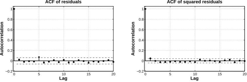
0 5 10 15 20

−0.2 0 0.2 0.4 0.6 0.8 1

Lag

Autocorrelation

ACF of residuals

0 5 10 15 20

−0.2 0 0.2 0.4 0.6 0.8 1

Lag

Autocorrelation

ACF of squared residuals

Fig. 5.

Autocorrelation function for ARMA-GARCH residuals for precipitation (1979–1993) of

Garmisch-Partenkirchen (top), and its corresponding squared residuals (bottom).

39

Fig. 5. Autocorrelation function for ARMA-GARCH residuals for precipitation (1979–1993) of Garmisch-Partenkirchen (left), and its corresponding squared residuals (right).

time series are substantially different from those of the re-gional climate model.

Both autocorrelation function and Ljung-Box Q-test are applied to test the performance of the ARMA-GARCH mod-els. The tests are applied to the original time series, the squared original time series as well as the resulting standard-ized residuals and standardstandard-ized squared residuals after ap-plication of the ARMA-GARCH model. According to the autocorrelation function plots the original time series of ob-served and RCM time series show serial dependence and het-eroskedasticity. This non-iid behaviour is illustrated exem-plarily for station Garmisch-Partenkirchen (Fig. 4). Figure 5 shows the autocorrelation function after application of the ARMA-GARCH model.

The Ljung-Box Q-test tests the data against the null hy-pothesis that a series of residuals exhibits no autocorrelation for a fixed number of lags against the alternative hypothesis that the autocorrelation is nonzero (Box et al., 1994). Table 4 demonstrates exemplarily the results of the Ljung-Box Q-test for the observed and modelled rainfall data (positive pairs) before and after application of a first order ARMA-GARCH model. All of the analyzed RCM rainfall time series are

af-fected by serial correlation for the lags 1, 5, 10, 15, and 25 days. After ARMA-GARCH transformation the RCM resid-uals exhibit no autocorrelation for the analyzed lags. For the observed time series, three different types of autocorrelation can be classified:

1. Strong persistent autocorrelation before, no autocorre-lation after application of ARMA-GARCH (90.15 % of all cases).

2. Strong persistent autocorrelation before, re-duced/remaining autocorrelation after application of ARMA-GARCH (7.58 % of all cases). In these cases higher order ARMA-GARCH models could further reduce the autocorrelation.

3. Weak persistent autocorrelation before, no autocorrela-tion after applicaautocorrela-tion of ARMA-GARCH (2.27 % of all cases).

The test results do not fully correspond to the au-tocorrelation functions (as shown for station Garmisch-Partenkirchen), however, both the graphical representations

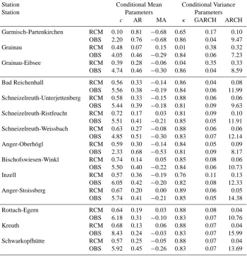
Table 2. Mean and standard deviation of the parameters for the fitted ARMA(1,1)-GARCH(1,1) models for selected stations (OBS) and their corresponding RCM grid cells (see Table 1 for further details about the stations). The conditional mean parameters of the ARMA model consist ofc, the conditional mean constant, AR, the conditional mean autoregressive coefficient, and MA, the conditional mean moving-average coefficient. The conditional variance parameters consist ofκ, the conditional variance constant, GARCH, the lagged conditional variance coefficient, and ARCH, the lagged residual coefficient.

Data source Conditional Mean Conditional Variance Parameters Parameters

c AR MA κ GARCH ARCH

RCM MEAN 0.57 0.27 −0.09 0.72 0.12 0.11

STD 0.16 0.18 0.20 0.30 0.11 0.10

OBS MEAN 5.18 0.45 −0.27 0.84 0.06 11.21

STD 1.57 0.13 0.17 0.02 0.02 2.48

Table 3. Parameters for the fitted ARMA(1,1)-GARCH(1,1) models for selected stations (OBS) and their corresponding RCM grid cells (see Table 1 for further details about the stations). The conditional mean parameters of the ARMA model consist ofc, the conditional mean constant, AR, the conditional mean autoregressive coefficient, and MA, the conditional mean moving-average coefficient. The conditional variance parameters consist ofκ, the conditional variance constant, GARCH, the lagged conditional variance coefficient, and ARCH, the lagged residual coefficient.

Station Conditional Mean Conditional Variance

Station Parameters Parameters

c AR MA κ GARCH ARCH

Garmisch-Partenkirchen RCM 0.10 0.81 −0.68 0.65 0.17 0.10 OBS 2.20 0.76 −0.68 0.86 0.04 9.47

Grainau RCM 0.48 0.07 0.15 0.01 0.38 0.32

OBS 4.05 0.46 −0.29 0.84 0.06 7.23

Grainau-Eibsee RCM 0.39 0.28 −0.06 0.04 0.35 0.33

OBS 4.74 0.46 −0.30 0.86 0.04 8.59

Bad Reichenhall RCM 0.56 0.33 −0.14 0.86 0.04 0.08

OBS 5.56 0.38 −0.19 0.84 0.06 11.99 Schneizelreuth-Unterjettenberg RCM 0.58 0.33 −0.15 0.88 0.06 0.06 OBS 5.44 0.39 −0.18 0.81 0.09 9.63 Schneizelreuth-Ristfeucht RCM 0.72 0.17 0.03 0.81 0.09 0.10 OBS 5.51 0.41 −0.21 0.85 0.05 11.91 Schneizelreuth-Weissbach RCM 0.63 0.27 −0.08 0.88 0.06 0.06 OBS 4.85 0.51 −0.30 0.83 0.07 12.14

Anger-Oberh¨ogl RCM 0.59 0.30 −0.14 0.84 0.05 0.09

OBS 2.33 0.68 −0.53 0.81 0.09 8.17 Bischofswiesen-Winkl RCM 0.74 0.14 0.05 0.85 0.08 0.06 OBS 5.50 0.40 −0.22 0.84 0.06 10.73

Inzell RCM 0.57 0.36 −0.19 0.76 0.11 0.13

OBS 6.05 0.42 −0.20 0.82 0.08 12.33

Anger-Stoissberg RCM 0.67 0.20 0.00 0.89 0.06 0.05

OBS 5.74 0.41 −0.21 0.85 0.05 14.38

Rottach-Egern RCM 0.64 0.19 0.03 0.88 0.08 0.04

OBS 6.18 0.31 −0.10 0.83 0.07 10.76

Kreuth RCM 0.68 0.13 0.06 0.88 0.07 0.04

0.0 0.2 0.4 0.6 0.8 1.0 0.0

0.2 0.4 0.6 0.8 1.0

Wi :n HH

i

L

0.0 0.2 0.4 0.6 0.8 1.0

0.0 0.2 0.4 0.6 0.8 1.0

Wi :n HH

i

L

Fig. 6. K-plot of the observed rainfall time series at station Garmisch-Partenkirchen (Germany) before

ARMA-GARCH transformation (top), and after ARMA-GARCH transformation (bottom).

Superim-posed on the graph are a straight line (blue) corresponding to the case of independence and a curve

corresponding to perfect positive dependence (red).

40

Fig. 6. K-plot of the observed rainfall time series at station Garmisch-Partenkirchen (Germany) before ARMA-GARCH transformation (left), and after ARMA-GARCH transformation (right). Superimposed on the graph are a straight line (blue) corresponding to the case of independence and a curve corresponding to perfect positive dependence (red).

Table 4. Ljung-Box Q-test results for three observation stations and their corresponding RCM grid cells. The test indicates whether or not the time series exhibit autocorrelation for a given number of lags [days]. One tests the null hypothesis that a series exhibits no autocorrelation for a fixed number of lags against the alternative hypothesis that the autocorrelation is nonzero. “1” indicates that the null hypothesis is rejected (i.e. autocorrelation), and “0” indicates no autocorrelation for any given time lag and level of significance (significant atα= 0.05 (normal font), orα= 0.01 level of significance (bold)).

Station without ARMA-GARCH with ARMA-GARCH

1 5 10 15 20 1 5 10 15 20

Anger-Oberh¨ogl RCM (original) 1 1 1 1 1 0 0 0 0 0

RCM (squared) 1 1 1 1 1 0 0 0 0 0

OBS (original) 1 1 1 1 1 0 0 0 0 0

OBS (squared) 1 1 1 1 1 0 0 0 0 0

Grainau RCM (original) 1 1 1 1 1 0 0 0 0 0

RCM (squared) 1 1 1 1 1 0 0 0 0 0

OBS (original) 1 1 1 1 1 1 1 1 0 0

OBS (squared) 1 1 1 1 1 0 0 0 0 0

Garmisch-Partenkirchen RCM (original) 1 1 1 1 1 0 0 0 0 0

RCM (squared) 1 1 1 1 1 0 0 0 0 0

OBS (original) 1 1 0 0 0 0 0 0 0 0

OBS (squared) 0 0 0 0 0 0 0 0 0 0

and the test results show the same trends, i.e. ARMA-GARCH is capable to remove large parts of serial depen-dence. Even though higher order ARMA-GARCH models could improve the results for about 8 % of all stations, a first order ARMA-GARCH model is preferred to guaranty for consistency and comparability between the stations.

Figure 6 shows the K-plot of observed and modelled time series before and after the ARMA-GARCH transformation visualizing their dependence structure over the whole range of the data. The K-plots indicate that the untransformed data sets reveal positive dependence within the low ranks which is removed after application of the ARMA-GARCH transfor-mation. The remaining positive dependence in the upper tails of the residuals is the “real” underlying dependence between the two variables.

From the sensitivity experiment mentioned above, it is found that the larger the wet day threshold, the higher is the distortion of the upper tails after the ARMA-GARCH trans-formation, i.e. the smaller is the fraction of “artificial” de-pendence which has to be removed. This is due to the fact that the high values (extremes) are intrinsically already iid. The POT and the order of the ARMA-GARCH models are less sensitive to this effect. Further information about how to calculate and to interprete the K-plots can be obtained e.g. by Genest and Favre (2007).

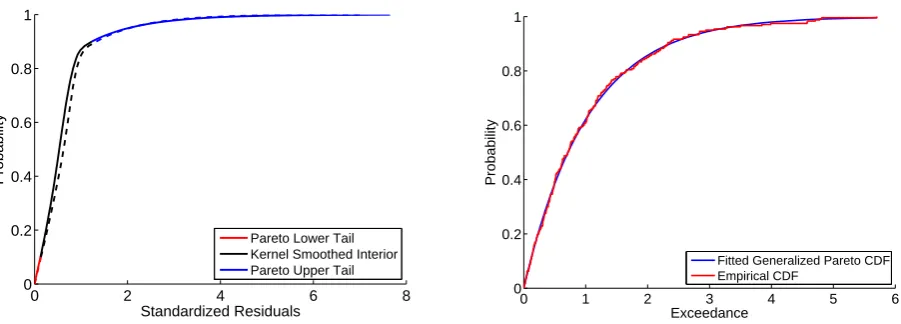
Figure 7 (left) shows the empirical and fitted exceedance probability for the upper tail of the observed rainfall residuals at station Garmisch-Partenkirchen. Both, for observed and modelled rainfall, the Generalized Pareto Distribution seems to be a good choice to fit the upper tails of the data. Figure 7

0 1 2 3 4 5 6 0

0.2 0.4 0.6 0.8 1

Exceedance

Probability

Fitted Generalized Pareto CDF Empirical CDF

0 2 4 6 8

0 0.2 0.4 0.6 0.8 1

Standardized Residuals

Probability

Pareto Lower Tail Kernel Smoothed Interior Pareto Upper Tail

Fig. 7. Empirical and fitted exceedance probability of the upper tail of observed rainfall residuals (top),

composite of the piecewise CDF of the modelled (solid lines) and observed (dashed lines) rainfall

resid-uals at Garmisch-Partenkirchen (bottom).

41

0 1 2 3 4 5 6

0 0.2 0.4 0.6 0.8 1

Exceedance

Probability

Fitted Generalized Pareto CDF Empirical CDF

0 2 4 6 8

0 0.2 0.4 0.6 0.8 1

Standardized Residuals

Probability

Pareto Lower Tail Kernel Smoothed Interior Pareto Upper Tail

Fig. 7. Empirical and fitted exceedance probability of the upper tail of observed rainfall residuals (top),

composite of the piecewise CDF of the modelled (solid lines) and observed (dashed lines) rainfall

resid-uals at Garmisch-Partenkirchen (bottom).

41

Fig. 7. Empirical and fitted exceedance probability of the upper tail of observed rainfall residuals (left), composite of the piecewise CDF of the modelled (solid lines) and observed (dashed lines) rainfall residuals at Garmisch-Partenkirchen (right).

(right) illustrates the composite of the three piecewise CDFs for modelled and observed rainfall residuals. It can be clearly seen that lower/upper tail as well as the interior of the distri-bution are fitted reasonably well to the observed data.

4.2 Analysis of empirical and theoretical Copula models

Figure 8 (left) shows the empirical Copula density be-tween modelled and measured rainfall for station Garmisch-Partenkirchen. Only the positive pairs of modelled and mea-sured rainfall are shown using a threshold of 0.01 mm to de-fine a wet day. It can be seen from the figure that the dis-tribution is strongly asymmetrical for the opposite diagonal of the unit square, and that the density in the upper corner is highest. This implies that modelled and observed rainfall are strongly concordant in the higher ranks of the distribu-tion, whereas the concordance is weaker in the lower ranks. This empirical density structure may be remarkably differ-ent compared to the ARMA-GARCH transformed residuals (Fig. 8, right).

Table 5 shows the results for the goodness-of-fit (GOF) test statistics using the parametric bootstrap procedure. In order to chose between the three different Copula families, namely Normal, Gumbel-Hougaard, and Clayton Copula, the parametric bootstrap algorithm of Genest and Remil-lard (2008) is applied to the residuals of observed and mod-elled precipitation. Although desirable in the long run, other promising theoretical Copula models such as the survival Clayton Copula are not considered in this study.

1000 bootstrap values of the Cram´er-von-Mises test statis-tic are produced, and the proportion of those values that are larger than Sn (p-values) is estimated. From the

p-values obtained the usability of the Gumbel-Hougaard Cop-ula is concluded. The CopCop-ula parameters which are used

for Copula-based stochastic simulations are also given in Table 5.

4.3 Dependence on large-scale weather situation

The dependence structure between modelled and observed rainfall, given the large-scale weather situation, is analysed. The method used for classifying large-scale weather types is described in Sect. 3.3. The empirical Copulas are calculated using different grouping strategies for the WTs. Based on the empirical Copulas, as well as the conditional CDFs, the usability for conditional simulations is investigated.

Using four different weather types and one indefinite type for advection (Fig. 9) can have additional value, and thus be used for conditional stochastic simulations. Figure 10 illustrates the empirical Copula density for modelled and observed precipitation for Garmisch-Partenkirchen group-ing the weather types due to the cyclonality in 950 hPa and 500 hPa into four classes. One can observe that for the four classes significant differences within the dependence structure between modelled and observed rainfall exist. The classification due to the humidity of the troposphere (Fig. 11) does not lead to a clear discrimination between the empir-ical Copulas. Both, the wet and the dry Copula density is similar to the unconditional Copula densities (compare with Fig. 8). The empirical CDFs of observed precipitation in Garmisch-Partenkirchen based on a given WT and certain groups of WTs are illustrated in Fig. 12. The performance skill of unconditional compared to WT conditional simula-tions of pseudo-observasimula-tions is demonstrated in the sequel. 4.4 Conditional stochastic simulations of

pseudo-observations

Fig. 8. Empirical Copula density for modelled (

u

) and observed precipitation (

v

) for station

Garmisch-Partenkirchen, using the positive pairs of original data (top), and the positive pairs of the

ARMA-GARCH transformed iid residuals (bottom).

42

Fig. 8. Empirical Copula density for modelled (u) and observed precipitation (v) for station Garmisch-Partenkirchen, using the positive pairs of original data (left), and the positive pairs of the ARMA-GARCH transformed iid residuals (right).

Fig. 9. Empirical Copula density for modelled (u) and observed precipitation (v) for Garmisch-Partenkirchen, using the weather type classi-fication following the advection of air masses. The advection types correpond to: (a) Northeast, (b) Southeast, (c) Southwest, (d) Northwest, and (e) no prevailing direction. The white areas originate from interpolation effects using an ordinary kriging algorithm.

that the modelled RCM precipitation is given (unconditional case). A split-sampling approach is used to subdivide the data into calibration and validation period. It can be seen from the figure that the observations are usually underpre-dicted by the model, and that the Copula-based technique can partly correct for that effect. For the very high RCM rainfall amounts, the Copula-based approach tends to overestimate

the observations. After this first graphical comparison the improvements attained using the Copula approach are ana-lyzed further with selected performance measures. A first hint of the skill is given by different error measures and e.g. the Pearson correlation coefficients between observations, RCM and the pseudo-observations, i.e. the bias corrected predictions (Table 6). The Pearson correlation coefficient

Fig. 10. Empirical Copula density for modelled (

u

) and observed precipitation (v) for

Garmisch-Partenkirchen, using the weather type classification following the cyclonality in 950 hPa and 500 hPa

respectively: (a) AA, (b) AC, (c) CA, and (d) CC (A – anticyclonic, C – cyclonic).

44

Fig. 10. Empirical Copula density for modelled (u) and observed precipitation (v) for Garmisch-Partenkirchen, using the weather type classification following the cyclonality in 950 hPa and 500 hPa respectively: (a) AA, (b) AC, (c) CA, and (d) CC (A – anticyclonic, C – cyclonic).

Fig. 11. Empirical Copula density for modelled (

u

) and observed precipitation (

v

) for

Garmisch-Partenkirchen, using the weather type classification following the humidity of the troposphere: (a) D,

and (b) W (D – dry, W –wet).

Fig. 11. Empirical Copula density for modelled (u) and observed precipitation (v) for Garmisch-Partenkirchen, using the weather type classification following the humidity of the troposphere: (a) D, and (b) W (D – dry, W –wet).

between observations and the mean value of the random sam-ple, generated through the Copula approach is 0.36. Please note that the correlation coefficient between observations and RCM is calculated as 0.3 for the iid transformed data of Garmisch-Partenkirchen. This corroborates the usability of the Copula based bias correction of precipitation.

Including large-scale information about advection, cyclon-ality, and humidity is increasing (decreasing) the correlation (deviation) between observations and pseudo-observations (see Table 6). The correlation between the RCM and the pseudo-observations is intrinsically high because the RCM data is used to constrain the Copula model. However, the Pearson correlation coefficient and the other used error mea-sures are just global meamea-sures, operating on the complete

Table 5. Goodness-of-fit (GOF) test using the Cram´er-von-Mises test statistics and parametric bootstrap procedure (see Sect. 3.2.2). p-values exceeding 0.01 are highlighted in bold.

Station Normal Copula Gumbel-H. Copula Clayton Copula

Sn p-value θN Sn p-value θGH Sn p-value θC

Garmisch-Partenkirchen 0.09 0.00 0.08 0.12 0.00 1.09 0.17 0.00 0.01

Grainau 0.10 0.00 0.09 0.15 0.00 1.10 0.16 0.00 0.01

Grainau (Eibsee) 0.07 0.00 0.12 0.08 0.00 1.11 0.12 0.00 0.06

Bad Reichenhall 0.10 0.00 0.19 0.04 0.02 1.15 0.37 0.00 0.13

Schneizlreuth-Unterjettenberg 0.14 0.00 0.15 0.10 0.00 1.13 0.29 0.00 0.08 Schneizlreuth-Ristfeucht 0.11 0.00 0.17 0.05 0.00 1.14 0.40 0.00 0.09 Schneizlreuth-Weissbach 0.08 0.00 0.13 0.06 0.00 1.11 0.21 0.00 0.07

Anger-Oberh¨ogl 0.10 0.00 0.16 0.05 0.01 1.14 0.34 0.00 0.11

Bischofswiesen-Winkl 0.07 0.00 0.16 0.04 0.07 1.14 0.23 0.00 0.11

Inzell 0.08 0.00 0.16 0.05 0.01 1.13 0.24 0.00 0.13

Anger-Stoissberg 0.12 0.00 0.14 0.06 0.00 1.12 0.40 0.00 0.07

Rottach-Egern 0.05 0.00 0.17 0.03 0.09 1.14 0.21 0.00 0.13

Kreuth 0.06 0.00 0.12 0.06 0.00 1.10 0.17 0.00 0.06

Schwarzkopfh¨utte 0.05 0.01 0.15 0.03 0.07 1.12 0.22 0.00 0.12

Table 6. Performance measures between positive pairs of pseudo-observations (mean value) produced by Copula-based stochastic simu-lations without using large-scale information (uncond), including advection (advec), cyclonality (cyclo), and humidity (humi) of the tro-posphere, and the observed precipitation at station Garmisch-Partenkirchen and the corresponding grid cell precipitation of RCM (RMSE – Root mean squared error; MAE – Mean absolute error; ME – Mean error; NSE – Nash-Sutcliffe efficiency; PCC – Pearson correlation coefficient).

uncond advec cyclo humi RMSE [mm d−1] observed 18.04 23.95 16.06 52.81

RCM 21.49 27.82 19.84 56.06

MAE [mm d−1] observed 3.13 3.21 2.98 3.41

RCM 3.40 3.48 3.29 3.59

ME [mm d−1] observed −3.00 −5.39 −4.13 −6.20 RCM −11.59 −12.12 −10.82 −12.90

NSE[−] observed 0.08 0.13 0.14 0.08

RCM −0.30 −0.18 −0.32 −0.04

PCC[−] observed 0.36 0.43 0.45 0.37

RCM 0.98 0.93 0.98 0.65

time series, and do not mirror the quality of the new method for specific subsets of the rank space. In turn, the probability plot (Fig. 14) provides a performance measure for the quan-tiles of the distribution.

It can be seen from Fig. 14 that the RCM underestimates the observations over the whole range of the distribution. Taking this as a reference, the Copula-based stochastic sulations of the pseudo-observations lead to significant im-provements. Including large-scale conditional information contributes moderately to a reduction of the bias.

5 Discussion

The bivariate dependence structure between RCM model output and gauge observations (RCM>0, gauge>0) is stud-ied to correct the systematic errors in the RCM simulations. In general there are four cases to distinguish, namely (0,0), (1,0), (0,1) and (1,1) where 0 denotes a dry and 1 a wet day. A wet day is defined as a day of rainfall≥0.01 mm which is chosen due to the minimum resolution of rain gauge mea-surements. Although the gauge measurements are affected by different sources of measurement errors such as errors due to wind or evaporation, they are treated as a reference for the “true” precipitation.

0 20 40 60 80 100 0 0.2 0.4 0.6 0.8 1

precipitation amount [mm]

Probability

Northeast Southeast Southwest Northwest

no prevailing direction

0 20 40 60 80 100

0 0.2 0.4 0.6 0.8 1

precipitation amount [mm]

Probability

AA AC CA CC

0 20 40 60 80 100

0 0.2 0.4 0.6 0.8 1

precipitation amount [mm]

Probability

D (dry) W (wet)

Fig. 12. Empirical CDF of observed precipitation in Garmisch-Partenkirchen, conditioned on the

occur-rence of (i) four different advection types plus one unspecified type, (ii) the following cyclonality types

in 950 hPa and 500 hPa respectively: AA, AC, CA, and CC (A – anticyclonic, C – cyclonic), and (iii) the

following humidity types of the troposphere: D, and W (D – dry, W – wet). Dry (wet) types are colored

red (blue).

46

0 20 40 60 80 100

0 0.2 0.4 0.6 0.8 1

precipitation amount [mm]

Probability

Northeast Southeast Southwest Northwest

no prevailing direction

0 20 40 60 80 100

0 0.2 0.4 0.6 0.8 1

precipitation amount [mm]

Probability

AA AC CA CC

0 20 40 60 80 100

0 0.2 0.4 0.6 0.8 1

precipitation amount [mm]

Probability

D (dry) W (wet)

Fig. 12. Empirical CDF of observed precipitation in Garmisch-Partenkirchen, conditioned on the

occur-rence of (i) four different advection types plus one unspecified type, (ii) the following cyclonality types

in 950 hPa and 500 hPa respectively: AA, AC, CA, and CC (A – anticyclonic, C – cyclonic), and (iii) the

following humidity types of the troposphere: D, and W (D – dry, W – wet). Dry (wet) types are colored

red (blue).

Fig. 12. Empirical CDF of observed precipitation in Garmisch-Partenkirchen, conditioned on the occurrence of (i) four different advection types plus one unspecified type, (ii) the following cyclon-ality types in 950 hPa and 500 hPa respectively: AA, AC, CA, and CC (A – anticyclonic, C – cyclonic), and (iii) the following humid-ity types of the troposphere: D, and W (D – dry, W – wet). Dry (wet) types are colored red (blue).

RCMs are known to produce a high number of rainy days with very small rainfall amounts which are not measured on the ground. These artifacts are eliminated by the thresh-old value. The case (0,1), where the RCM misses a rainy day cannot be corrected by this approach and has to be

Fig. 13. Copula-based stochastic simulations of 50 consecutive positive pairs (precipitation>0.01 mm) performing 100 realizations (illustrated as box-whiskers) ofV (observed rainfall at gauge, illustrated as red line) assuming thatU (corresponding coarse scale MM5 precipitation, illustrated as black line) is known. The boxes have lines at the lower Q1 and upper quartile Q3 and the median values Q2 (middle horizontal lines). The whiskers (vertical lines) are lines extending from each end of the boxes to show the extent of the rest of the data. The maximum length of the whiskers is determined by 1.5 (Q3–Q1). Outliers (crosses) are data with values beyond the ends of the whiskers.

47

Fig. 13. Copula-based stochastic simulations of 50 consecutive pos-itive pairs (precipitation>0.01 mm) performing 100 realizations (illustrated as box-whiskers) ofV (observed rainfall at gauge, il-lustrated as red line) assuming thatU(corresponding coarse scale MM5 precipitation, illustrated as black line) is known. The boxes have lines at the lower Q1 and upper quartile Q3 and the median values Q2 (middle horizontal lines). The whiskers (vertical lines) are lines extending from each end of the boxes to show the extent of the rest of the data. The maximum length of the whiskers is de-termined by 1.5 (Q3–Q1). Outliers (crosses) are data with values beyond the ends of the whiskers.

0.0 0.2 0.4 0.6 0.8 1.0 0.0 0.2 0.4 0.6 0.8 1.0 m odel o b s e rv a ti o n s hum i cy clo adv ec uncond obs

Fig. 14. Probability plots of observed and modelled precipitation time series at station

Garmisch-Partenkirchen. If the quantiles of the two distributions agree, the plotted points fall on exactly on the

thin dotted line. The red quadrates illustrates the agreement between observed and RCM rainfall. The

black quadrates correspond to the Copula-based stochastic simulations without additional large-scale

information. The Copula-based simulations including advection, cyclonality, and humidity of the

tropo-sphere are illustrated as blue, green, and orange quadrates respectively.

48

Fig. 14. Probability plots of observed and modelled precipitation time series at station Garmisch-Partenkirchen. If the quantiles of the two distributions agree, the plotted points fall on exactly on the thin dotted line. The red quadrates illustrates the agreement between observed and RCM rainfall. The black quadrates correspond to the Copula-based stochastic simulations without additional large-scale information. The Copula-based simulations including advection, cyclonality, and humidity of the troposphere are illustrated as blue, green, and orange quadrates respectively.

0 10 20 30 40 50 60 0

0.2 0.4 0.6 0.8 1

precipitation amount [mm]

Probability

CP39, SWCCW (wet) CP2,

NEAAD (dry)

Fig. 15. Empirical CDF of observed precipitation in Garmisch-Partenkirchen, conditioned on the

oc-currence of the Northeast advection type WT 2 (NEAAD), and the Southwest advection type WT 39

(SWCCW).

49

Fig. 15. Empirical CDF of observed precipitation in Garmisch-Partenkirchen, conditioned on the occurrence of the Northeast ad-vection type WT 2 (NEAAD), and the Southwest adad-vection type WT 39 (SWCCW).

investigated separately. Please note that the positive pairs are not consecutive except for certain periods, threrefore the described simulation process does not produce a continuous time series.

In literature the fact that positive pairs are usually non-consecutive has often been used to justify the assumption of iid behaviour (e.g. Villarini et al., 2008), mainly neglecting serial autocorrelation. For the modelling of extremes iid be-haviour is commonly justified by reducing the sample size using block maxima or peaks over threshold methods. Al-though the focus lies on modelling of positive pairs of daily precipitation values (observations and RCM), a different ap-proach is required as it is found that they are non-iid. More detailed they are affected by non-stationary of mean and vari-ance (volatility). Simple models such as AR, MA, ARMA, or GARCH fail to eliminate both effects at the same time. Therefore, combined ARMA-GARCH models are used in this study.

As extreme values are known to have different marginals compared to the rest of the data, a GPD distribution is used in this study. This distribution allows for separately modelling upper and lower tail and interior of the empirical distribu-tion and thus for extrapoladistribu-tion of the extreme values. This approach is superior insofar as it gives the same weight to each part of the data, albeit the tails hold a smaller cardinal-ity than the interior.

The remaining residuals are not affected by serial correla-tion and variance clustering and offer the possibility to study the “real” underlying dependence structure between two (or more) variables which are described by copula functions. It could be shown that the empirical copula functions be-tween the two original time series are remarkably different from those obtained by the residuals of the ARMA-GARCH models. Filtering the time series before fitting to a

the-oretical Copula model is reducing the correlation between RCM (here: MM5) and observed precipitation and thus the estimated Copula parameter θ, which is directly related to Kendall’sτ. Serial correlation within the single time series can artificially disturb the joint dependence structure.

From the theoretical Copula models analyzed, the Gumbel-Hougaard Copula is found to be a suited choice to model the joint distribution of modelled (gridded) and ob-served precipitation. While the Copula parameter is rela-tively stable for the joint distribution functions between dif-ferent locations within the same grid cell, the shape and scale parameters of the fitted marginal distributions of the observa-tion staobserva-tions can differ significantly. The scale parameters of the observations are significantly greater than those of the RCM simulations indicating to remarkably higher variances in the observation series.

The empirical Copula density plots are used to analyze the dependence structure between modelled and observed pre-cipitation. As computational inexpensive they are suitable to (i) find a theoretical Copula model, and (ii) screen variables such as e.g. large-scale weather types which could addition-ally improve the performance of the bias correction. It must be mentioned critically at this stage that only three differ-ent theoretical Copula models are tested. These models are capable to reproduce asymmetries along the major diagonal of the dependence structure. This cannot be achieved using a Gaussian approach. The observed empirical Copulas also show asymmetries along the minor diagonal, which are still not captured by the theoretical Copulas. Copula functions accounting for these asymmetries could further improve the results.

The objective weather pattern classification method of the German Weather Service (Bissolli and Dittmann, 2001) is used to further constrain the model. As the usage of 40 differ-ent weather types would not lead to sufficidiffer-ent sample sizes, needed for statistically significant inferences, three different grouping strategies were used (see Sect. 3.3). This leads to a sufficiently large sample sizes (average of∼400 members for each subgroup) to guarantee for statistical significance.

To demonstrate the “added value” for the bias correction by means of weather classification the marginal distributions as well as empirical Copulas are shown for each classified group. A comparison of the CDFs shows that a clear discrim-ination between the different subgroups, such as e.g. dry/wet troposphere is achieved. The empirical Copula functions also show a clear discriminative power, especially for direction of the advection of air masses at 700 hPa and cyclonality at 950

hPa and 500 hPa. A decision about the improvements of the

simulated pseudo-observations using weather classifications, solely based on differences in the CDFs or empirical Cop-ula densities alone is difficult. Including information about the humidity of the troposphere can slightly increase the skill for bias correction compared to the Copula-based stochastic simulations without using large-scale information. This can be seen from the conditional CDFs and the corresponding

0 200 400 600 800 1000 0.35

0.4 0.45 0.5 0.55 0.6 0.65 0.7

time step (positive pairs)

τ

Fig. 16. Kendall’s

τ

of 101 consecutive positive pairs for modelled and observed precipitation at station

Garmisch-Partenkirchen.

50

Fig. 16. Kendall’sτof 101 consecutive positive pairs for modelled and observed precipitation at station Garmisch-Partenkirchen.

probability plots for the different groups, which are not very discriminative (compare Sects. 3.3 and 4.4). Using the sin-gle 40 weather types (without grouping) could potentially increase the discriminative power (see e.g. Fig. 15), but de-creases the sample size of certain WTs far too much to reli-ably estimate the Copula parameter(s) and the marginal dis-tributions.

Another limitation of the approach shown in this paper is that the same theoretical Copula model, i.e. the Gumbel-Hougaard Copula, is fitted to each WT class. It is obvious from the empirical Copula density plots, that this does not necessarily provide an adequate fit for all groups of weather types. It is also well-known from other studies that the do-main size (here: whole Central Europe dodo-main) can strongly impact the classification results (e.g. Laux, 2009), and thus the subsequent conditional modelling.

In this study a stationary approach for the Copula param-eterθis chosen. Further improvements are expected by ac-counting for the temporal variability ofθsuch as e.g. demon-strated in the the paper of Reboredo (2011). Figure 16 il-lustrates the temporal variability ofτ, which is empirically linked with the Copula parameter. As seen in Sects. 4.2 and 4.4, all the empirical Copulas derived in this study show a strong asymmetry with respect to the minor axisu= 1−vof [0,1]2. This asymmetry can not be depicted by the common Copula families such as the Clayton, Normal or Gumbel-Hougaard Copulas, acting as basic set of possible candidates for the performed GOF tests. Nonmonotonic transformation to construct asymmetric multivariate Copulas from the Gaus-sian (B´ardossy, 2006) could reflect the asymmetries in the empirical Copulas and thus also improve the bias correction.

6 Conclusions

The presented Copula-based approach is potentially useful for statistical downscaling, bias correction, and local refine-ment of RCMs. The performance will be evaluated and com-pared to established methods for bias correction.

Asymmetries are found in the empirical Copula densities which cannot be reproduced by the theoretical Copulas used in this study. Therefore, it is generally difficult to find a the-oretical Copula model which is not rejected by the applied GOF test.

Fitting the marginal distributions is of crucial impor-tance as it strongly impacts the simulation results (more than the Copula parameter θ). It could be shown that iid transformations such as ARMA-GARCH are indispens-able before a mutual dependence structure between vari-ables on daily scale is modelled to avoid artefacts induced by autocorrelation.

Large-scale weather patterns could be used to further con-strain the model, and thus, increase the performance of the simulation results.

Acknowledgements. This research is funded by the Bavarian State Ministry of the Environment and Public Health (reference number VH-ID:32722/TUF01UF-32722). Additional funding by the Federal Ministry of Education and Research (research project: Land Use and Climate Change Interactions in Central Vietnam LUCCi, reference number 01LL0908C), by the HGF Impuls-und Vernetzungsfond (research project: Regional Precipitation Observation by Cellular Network Microwave Attenuation and Application to Water Resources Management PROCEMA, Virtual Institute, reference number VH-VI-314), and by HGF (research project: Terrestrial Environmental Observatories TERENO – http://www.tereno.net) is highly acknowledged. The help of Thomas Rummler, who created Fig. 2 is appreciated.

Edited by: C. Michele

References

AghaKouchak, A., B´ardossy, A., and Habib, H.: Copula-based uncertainty modeling: Application to multi-sensor pre-cipitation estimates, Hydrol. Process., 24(15), 2111–2124, doi:10.1002/hyp.7632, 2010a.

AghaKouchak, A., B´ardossy, A., and Habib, H.: Conditional sim-ulation of remotely sensed rainfall data using a non-gaussian v-transformed copula, Adv. Water Resour., 33(6), 624–634, doi:10.1016/j.advwatres.2010.02.010, 2010b.

B´ardossy, A.: Copula-based geostatistical models for groundwa-ter quality paramegroundwa-ters, Wagroundwa-ter Resour. Res., 42(11), W11416.1– W11416.12, doi:10.1029/2005WR004754, 2006.

B´ardossy, A. and Li, J.: Geostatistical interpolation using copulas. Water Resour. Res., 44(7), W07412.1–W07412.15, doi:10.1029/2007WR006115, 2008.