An Analytical and Experimental Study of High Velocity Flow in Curved Sections of Open Channels

T.

Submitted in Partial Fulfillment of the

for the

Institute of

Flood Control District under ef ""'~'·""""il"'"

C. H. for the financial side of

to state here his

The writer

of the many made the course of his

Professor R. T. and Professor Th. von deal of credit is due if this

a s forward in the science of

Mr.

E.

was connected with the construction

and the first of Messrs.

J.

M.

Fox and T.

w.

were

latter of work and. in the evaloo,tion on the amount

Of

data.

and. was members

of

the Los

• to mean

of

on.

the

and

SUMMARY

In the theory of flow in open channels two stages of flow with principall;:r different characteristics have to be considered, streaming flow and shooting flow. The velocity of flow in the first case is smaller than the velocity of propagation of trans-latory waves, in the latter case it is larger. The phenomena

occurring in streaming flmnr are well known and theoretically solved, if i'lre neglect the influence of friction. This latter simplification means that the velocity has a constant value for each point of

the cross-section. For this assumption also the theory of the hy-draulic jump has been successfully attacked, where the stage of

flO'w· changes i'rom the shootil1g to the s·treaming condition. The present paper, however, deals with problems of flow of the shoot-ing stage only and extends the theory of hydraulics to all cases of supercritical flow, where the variation of depths and velocities due to cha.11ges in the direction of' f'lovr is desired.

B. Analytical St::_dy. of Supercritical Flow

I. !_upercritical Flo'~

a. Definition of Supercritical Flow and Wave

Velocity b. Properties of Flow at Supercritical

Velocities c. Boundary of Disturbances

a. Derivation of Wave .Angle

b. ~:'he Influence of a Change in the Direc-tion of Flow

c ..

d.

1.

General

Law

2. Conditions for Application to Flow in Curves Derivation of Elevation Procluced by Change

in Direction

1. Discussion of Possible Assmnptions

2. Derhni:tion on the Basis of Constant Energy

3. Derivation on the Basis of Constant ·velocity Derivation of Location and Magnitude of

First ]\[J.aXimturL

1. Location of Beginning of First Maximum 2. Depth in Zone of First Maximum

I. Experimental Procedure

II. Schedule of Tests

III.

Graphical Results

a. Water Surface Contour Maps

b. Water Surface Profiles Along Channel

Walls

c. Water Surface Profiles Along Outer

Chan-nel Vi.alls

d. Cross-Sections of Flow and Velocity Distribution

2 .. 20

2 - 5

2

4

5

6 - 20

G

8

8

8

13 - 17

13

14

17

18 - 19 18

19

21 - 50

21 22

27 - 50

27 31

38

TABLE OF CONTENTS (cont.)

D. Comparison of Experimental and .Anal;rcical Results 51 - 64

I. Cow..parison of Jl..nalyti ce:?.- and Experimental 51 Profife .. ~Rise

II. Comparison of Analytical and Exper:i.mental - 54 - - - · ,,_ -~··-·-.. - · ~---· Maxima

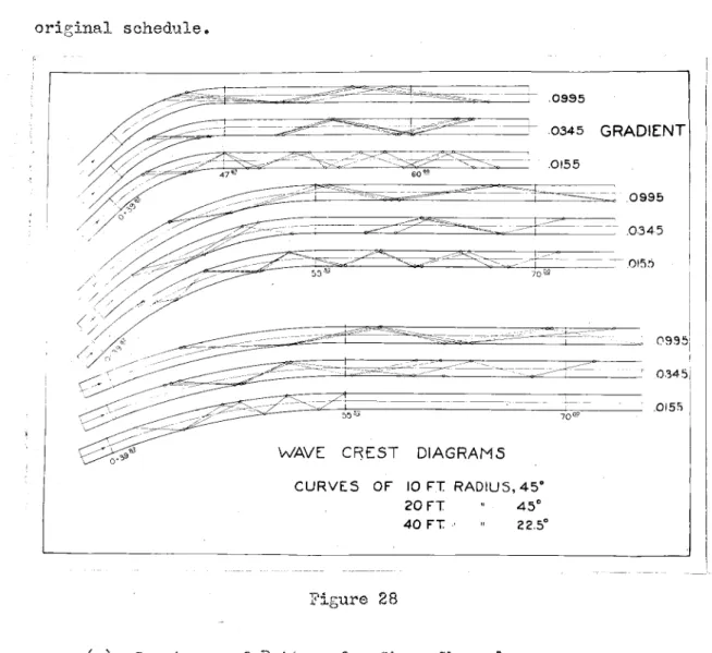
III. The General Pattern of Disturbances Setup - - 59 - · - - - · - · · - - By-·curves

a. Constancy of Pattern for a Given-Chanr1e1 60

b. The Spacing of Maxima 61

c. The Number of Maxima in Curve 61

d. Relative Height of' Ma.x;4na in Dovmstrea.m 62 Tangent

E. General Dj_scussion and Final Conclusions _{65 - 68}

I. The Experimental Set-Up

The Circulation System

a • The Discharge Measurement

b. The Tilting Platfonn

c. The Experirnen·bal Flume

d. Portable Testing Instruments II. Field Observations on_Flow in curves

a. Verdugo Wash High Water IvTarks b. Lower Sycamore Storm Drain

c. Rubio Storm Drain

d. Summary of li'ield Checks

III. A Short Survey of Literature on High Velocity Flow and on Flovv- in Curves at Subcri

ti

cal

Velocities

69 - 75

71

73

'73

74

'76 - 81

76

77

78

81

1. Specific Energy Diagram 2

2. Paths of Yfave Fronts 6

3. Velocity Vector Dia.gram for Constant Energy 15

Assumption

4. Velocity Vector Diagram. for Constant Velocity 17 .Assumption

5. Dia.grrun for Derivation of Location of First 19 lfaximu:r!l

Water Surface Contour Maps

6. Runs 13 and 39, Runs 3 and 32 28

7. Runs 19c and 28, Run 26 29

8.

Runs

52, 57 and 71 30

Water Surface Profiles Along Channel Yfalls

9. For 10 foot and 20 foot Radius of Curvature 32

10. For 40 foot Radius of Curve.ture 33

11.

For Runs

of l-l/2fa Slope 34

12. Photographs of Run 13 35

13. Photographs of Runs 11 and 39 36

14. Photographs of Run 32 37

Water Surface Profiles Along Outer Channel W"alls

15. For 10 foot and 20 foot Radius of Curvature 39

16. For 40 foot Radius of Curvature 40

17. For

Runs

of l-l/2;1a Slope 41

Cross-SectiOllll.s of Flow and Velocity Distributions

18. Runs 10 and 13 43

19. Runs 19c and 26 44

20. Runs 28 and 32 45

21 •• Run 39~ Runs 18 and 35-37 46

22. Runs 52 and 57 47

LIST OF FIGUP.ES .AND TlillLES

(cont.)

Figure.

24. Photographs of Run 180 49

25. Photograp~s of Runs 35 - 36 50

26. Photogra.ph of Shape of Rise 51

27. Diagram of Approximate Solution for Long Radius 59 Curves

28. Ylave Crest Diagrams 60

29. Photogra~hs of Disturbance in Dovmstream Tan- 63

gent, Slope 3-1/2%

30. Photographs of Disturbance in DoTunstrerun. Tan- 64 g;ent, Slope 1-1/2~~

31. Water Surface Profiles Along Channel Vfo.lls, 66

Compound Curves

32. Water Surface Profiles Along Outer Charm.el 67 Walls, Compound Curves

33. Diagram of Experimental Set-Up 69

34. Scale Dravring; of' Experimental Set-Up 70

35. 10" Venturi Neter 71

36. Venturi Manometer and Regulcling Valves 72

37. Slope Adjustment 73

38. Entrance Nozzle 74

39. Point Gimge 74

40. Pitot Measurement 75

41. Wall Profiles of Rubio '\'Tash 80

Tables

I. Complete List of Runs end Corresponding

Hydraulic Data

II. Cornparison of Shape of Rise in Depth Along Outer Wall III. Comparison of Iv'Iaximum. Depths at Outer Wall

24 - 26

52 - 53

d

=

variable local depth

d₀

=

critical depth

d₀

=

average depth in the channel of approach

h' • maximum depth at the outside wall of the curve

b

=

v-ridth of rectangular section

p • wetted perimeter

m

=

hydraulic radius

v₀

=

average velocity in channel of approach

v

=

varie.ble local velocity

v₀

=

c - critical velocity= vmve velocity or celerity

Q

=

tote.l discharge

q

=

discharge per unit width

s

=

slope of flume along centerline

g

=

acceleration of c;ravity

=

32.2 ft/sec2

n ::. Manning's coefficient of roughness

R • radius of cur-1rature of oenterli.ne of flume

9

=

e:ent~al angle of turn

9

0

=

central angle from begi:nning of curve to first maximur1

~ • variable local value of wave angle

1

A. INTRODUCTION

The investigation presented in the following started origin-ally as an experimental study, from which information was desired on the behaviour of flow at high velocities in curved sections of open channels. In order to simplify the approach to the problem, the cross-section of the channel vro..s chosen rectangular with zero cross-slope. The range of velocities to be considered was such that at any point the velocity stayed above the critical. For the latter condition, it was found, that the laws and formulae that are used and proven correct for lov; velocity flow failed to yield any resul-t;s consistent with the experimental outcome of the study.

The theory developed thus far for supercritical velocity deals only Vtli th straight flow and parallel streamlines or with the trans-_ition from the supercritical to the subcritical stage as encountered

in the hydraulic jump. In order to obtain a fundamentally correct basis for the analytical study of the problem of flow in curves at velocities which stay alvmys in the supercritical ran0e, the

B. ANALYTICAL STUDY OF SUPERCRITICAL FLOW

__

. . _ . . _ ...

~~-I. Supercritical Flow

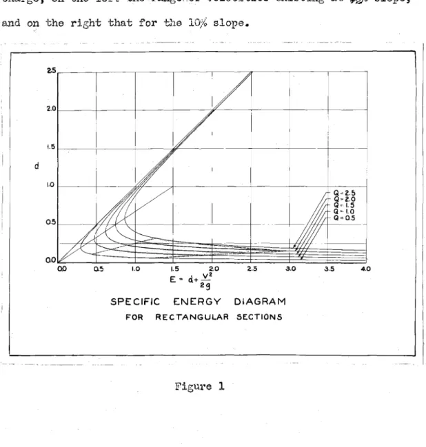
a. Definition of Supercritical Flow ~d ]~<:_!el?_<?_it~. The best illustration for the conditions existing at supercritical ve-locities is given in Fig. 1, which shows the v.rell-lplown specific energy diagram. plotted for the range of conditions as existed in the experimental investigation. The range covered by the experi-ments is indicated by the shaded area. The boundaries of this area are: On top and bottom the lines of :maximum and minimum dis-charge, on the left the range of velocities existing at

J.-?ffe

slope, and on the right that for the 10% slope.

d

0.5 1.0 1.5 2.0

E = d+ v2 29

2.5

SPECIFIC ENERGY DIAGRAM

FOR RECTANGULAR SECTIONS

Figure 1

3.0

Q 2.5

Q Q 2.0

1.5

Q 10 Q 0.5

3

This diagram ;vas obtained by plotting the specific energy

defined as

£

a s a function of the depth d • The eA1?ress~on for

E

can be modified, since

q

=

vd, to

(1)

E

=

d

For constant discharges

q

the curves show.n in Fig. l can then be

dravm. We find that above a certs.in line, where the slope of the

curves changes /1 all the curves approach as;ymptotically the stra.iGht

line E

=

d • The percentage of potential energy as expressed by

d in the above relation is here apparently the larcer one. If ti~e

depth diminishes the value of E depends more and more on ·the

second term in. the relation or, in other words, on the velocity·

head. The point, -<:1£ whare. inf1:aiatim:i. of Hie slope. the curvesYis seen cha•'l~QS to give the

minimum value for the specific enerf;Y E • We therefore obtain

it by differentiating E with respect to d and by putting the

derivative equal to zero. This gives v •

Vi!f.

The values of

d and v obtained by this process are called the critical depth

and the critical velocity, respectively. They are defined

there-fore as the dep·th and velocity at which a certain discharge can

f'low ·with the minimum amount of energy.

The significance of critical velocity for hydraulic problems

is augmented by the fact ·!:;hat it is approximately equal to the

velocity of propagation of waves. Ii' we assume the wave height

infinitely small,, the velocity of propagation becomes equal to

c ::

fgcf •

This relation is arrived at by applying the principle

.9...

v

9

+

+

If due to some disturbance the depth d is changed to D , the momentum v.rill be

=~

gO

+

•

equal, we have a state of equilibriu.r.i and the assumed disturbance, 11rhere we have the change from d to D , is stationary. We can

express this condition also in the followini; way: the velocity of propagation of the disturbance has become equal to the velocity of flo11v of the fluid entering into the zone of disturbance.

There-fore and since q •

d•v •

V·D

(2)

We see that only for the relation ~ a I we obtain

theoret-ically a velocity of propagation v :: c :: ( gD which may also be

called celerit;y. However, practically the m.un.erical value of

differs from U...'1.i ty only for

larg~

values of

~

• Therefore it is possible that for these cases a wave of large height as co:ntpared to the dep·bh ca:.'1 travel upst:rea:m even if the

velocity of flow is equal to a v somewhat above the critical value ir •

(id •

The critical velocity of flow and the veloci "bJ of propagation of shallow depth water waves coincide only if the wave height can be neglected with regard to the depth.

~-- P:i;:'?.12.~!..~~'.:..! of Flow at Supercritical Velocities. From the

5

of conclusions which are of' decisi-ve value for the problem in question. The most outstanding dif'ference between flows occurring above and below the critical stage is, that disturbances generally cannot be propagated upstream or, in other words, downs·trea,.'11

con-ditions cannot affect upstream. ones. The only exception to this rule are waves of large height for the reason discussed in the previous paragraph. Thus, for example, a pier or other obstruction in a stream flowing at superori ti cal veloc:U:;y cannot canse an

in-crease in depth at any point at any appreciable distance upstream

from the obstruction, unless it does so by causing the flow to

pass out of the supercritical range. When this does occur,

it

is shown by the presence of a hydraulic jump. Howeyer, if the flow does remain completely in the field of supercritical velocit"IJ, the

disturba...~ce is propagated in the direction of flow. This can be

represented by a disturbance propa{o;ated in all directions from the

obstruction with the wave velocity superimposed upon the velocit;y

of flow. Since this latter velocity is always greater than the

form.art there will be no resultant upstream. components. The limits

of the disturbance will be a V with the apeJc at the obstruction,

i.e. similar in appearance to the bow wave of a boat. The angle of. this

v

is equal to twice the wave angle.

c. Bound~~is~~r~a::_~~· The significance of this

only the change in the corn.ponent perpendicular to the 'Wave front

can produce a change of elevation. 'rhese unique properties of

supercri·i:;ical .flow hold the key to the solution of many of' its problems, of which the flow around curves is one.

PATHS OF 'WAVE FRONTS

CURVED FLOW

c=f9d ~ 2.6

STRAIGHT FLOW

Figure 2

II. Lav.rs Pertaininp; to Supercritical Flow

- - - :

a. Derivation of Wave ~gle. We are now in a position to

an-alyze the interrelations which mus·!:; exist in the case of corabined

flow of 11ro.ter and wave propagation. We know that a stone dropped

into still water will cause a circular wave travelling from the

7

imagine that a rectil:l.near flow superimposed on this cifcular wave

will distort the circular pattern., since the part of the wave

travelling upstrea:m will proceed with a resul"l:dnt; celeri"t'J of

fga -

v and the part directed downstree.m with the sum of the t-wo,

@

+

v If we accelerate the flow now to a point where

f"

id

=

v

=

c,

we see that the most the disturbance can do is to send a wave out

perpendicular to the direction of :Clow, while the celerity in the

downstream direction has become c

= 2

fid .

If the velocity of :flow

increases further, the disturbance will be propagated at an angle

P.,

to the direction of flow, given by the relation

!Jin.('.>

=

V

•

If the disturbance is a pennanent one and

the flow conditions are constant, the angle {2> stays constant too$

and we obtain a straight wave front progressing from the source

of di sturba.nce at an ai.'1gle

p.

with the direction of flow·, till it

is interfered with. If a wave hits a wall, it is reflected and travels back under the same angle

f-> •

If Jcwo waves cross each

other, they do not interfere, u11less the wa:l:;er flowing past a

wave front has suffered a change in direction or velocity due to a finite wave-height, then the wave crossing into a region of a

changed depth and velocity will proceed under a new angle deter-mined from the new values "{ gd and v •

In. the lower part of Fig. 2 is indicated a rectilinear flow

in a straight chaTu"J.el of constant velocity and depth. If we

cause e. small continuous disturba;."'1ce at the left entrance-section

these points will form. the diamond pattern indicated in the pic-ture.. Such patterns have been observed and photographed many times.

If nei~her the depth nor the velocity and its direction stay

constant, but vary as the wave progresses, the pattern of the waves is distorted accordingly and,, in the case of a curved flow, asslun.es the f'or:m shown in the upper part of Fig. 2.

b. The Influence of a Change in the Directio~-~·

1. General Law. The wave lines in Fig. 2 represent only waves of infinitely small size. If we have finite values of wave height,, the flow passing under such a wave will undergo a

change in velocity and depth in asreement with the law of con-servation of momentum. In this case the change of momentum of the

vmter passing the

wave

is therefore proportional to the change in depth. Further$ according to the derivation of the wave velocity, the direction of flow is perpendicular to the wave front, which

means that also the acceleration tL."lder a v:a-ve must be

perpendic-ular to the vvave front. If the direction of the flow is oblique

to the direction of the vmve front, only the component vn of the

velocity normal to the wave front can eni.~er into the problem,

while the tancential component vt remains unchanged. Expressing

these statements now in mathematical term.s, we have as a further

fundamental equation of our problem

( 3)

f

V-n. · 4 v"l't. - (' A cL

2. Conditions :for Application to Flow in Curves. 'rhe

previous discussion o:f the fundamental facts of supercritical

flow and of the mechanics of pressure translation will be extended

to the case of' flow· through curves., In the literature of Hydraulics

9

or supercritical, flo'V'r in curves. Only the case of lower than critical velocities in curved channels and river bends has been attacked and solved for certain assmnptions satisfying within cer-tain limits average natural conditions. The basic assur1ptions for the formula normally applied to curved flow are the following:

(a) the velocity of f'low is constant throughout the cross-section

(b) the direction of the strea.i.lllines is parallel to the 1valls (c) the velocity of propagation of the disturbance is greater

than the velocity of flow.

For

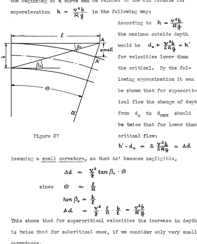
these assumptions we can arrive at a solution immediately11 since the only forces perpendicular to the flow in a curve a.re centrifugal force and counteracting it a static pressure force. Calling the difference of the depth at the outside and inside walls h 1 further assuming an average curvature of the

strewn-lines 1/R, we can write for a unit length of fluid the following

equa·!:;ion of' equilibrium: wherein h is

=

r·

ha

(4)

h

=

We see that according to the derivation not only the previously stated three assumptions have to hold, but also the superelevation h must be smal 1 as compared to the tota.1 depth d and b must be small against R •

the relation h, =

~,,~

can be maintained. We may with even better

accuracy introduce v • v $ since the velocity distribution mean

tends to become more a.~d more uni£orm with higher velocities.

The second assumption, however, of all the water moving par-allel to the walls cannot be :maintained any longer in the light of'

the previous discussion on the significance of the critical ve-locity a:nd wave velocity.

In changing the direction of a flowing stream we have to

accomplish a change of momentum. of the flowing vvater. This is

done by a pressure force proportional to a function of ·bhe angle of turn, £' (9) • This force is built up along the outside bank

of a stream, since the velocity vector there has a component

direc-ted toward the bank. The same happens a.long the inside ba.riJc with a :1egative sit_~ however, since the water has the tendency to flow

away from the bemlt. This is identical with ·!;he statement that

the beginning of a curve must be the beginning; of a ser:i.es of

in-fin.itesimal pressure disturbances near the two ·walls. Hemerr1bering that pressure changes ce.n only be tra.nsmit·ced to neighboring; sec-tions with a velocity equal to the 1;1J'ave v-eloci ty, we can express

the distinction between the cases of' curved flow above and below

the crit:i.cal velocity and find a new method of attack for curved

flovv at supe:rcri ti cal v·eloci ties.

11

stay approximately parallel to the bank and continue in curved

paths., The formul[1. derived above corresponds therefore to actual

conditions and gives.$ perhaps with some refinements, the true

value of h in this case.

In the ce.se of velocities of flow higher th.an the cri tica.l

we can state the problem. according to the foregoing discussion as

follows:

The pressure change along outer and inner vm.11 at the beginning

of a curve cannot be communicated over the entire section at once.

It

reaches neighboring strea:rr~ubes only at points dovmstream, lying along the imaginary wave front.$ which forms an angle

(3

with the

direction of flow as discussed before. .Any particle in the stream

will therefore keep its direction of flow until

it

passes under a wave front, where it becomes subject to ar1 acceleration normal to

this wave front. The particles moving alon.e~ the centerline stay

longest undisturbed.

The acceleration force affecting a particle passing under a wave front can be negative or positive,,, the component, vn , norm.al

to the wave :t'ront can be increased or decreased and accordingly

the depth below the wave may be higher or lower. This depends only

on the boundary conditions.

It

is evident that a vro.11 curving toward the center of the stream, and therefore obstructing the

flow, will cause deceleration of the flow and incree.se of depth,

while a wall curving avray from the stream_, allovtlng thereby an

depth. Correspondingly we may call these wave lines along v<l1ich

a constant impulse is transmitted from the boundaries,

"compres-sion" and 11_{depression waves". A curved channel will give rise to}

both kinds; compression waves along the outer wall and depression

waves e.long the inner wall. Both compression and depression waves

cross the stream and ultimately reach the opposite walls. Since the compression waves give an acceleration toward the wave front

a..n.d ca.use an increasing depth, successive waves must converge and

the surface slope must become steeper. The depression vvaves have

the opposite properties and therefore successive vmves diverse,

and the su:d'ace slope becomes flatter. In the case of curved

channels the two kinds of waves are started on opposite sides and

therefore they both turn ·the streamlines in the same direction.

This means that after they intersect the effect of the direction

change of the streamlines is added up8 while the influence on the

depth by one wave is counteracted by that of the other.

The practical application of this to our problem is the

follow-ing: The depth ;vill rise along the outer wall and decrea.se along

the inner wall until the waves, which started due to the beginning

of curvature at the respective opposite ~~lls, have completed

cross-ing the strewn. From this point of intersection of wave and wall,, the depth change must continue with a. reversed sign.

According to this discussion and forraer statements we are now

in a position to determine by mathematical approach the following

• .i..

l. ... ems:

13

the curve (also the corresponding drop along inner wall)

(b) the location of the beginning of the maximum depth

range

(c) the magnitude of ·i:;he maximum depth to be expected at

the outer iNB.11 of a curve.

1. Discussion of' Possible Assumptions. Before we enter into the mathematical derivations, we must gain a somewhat clearer

conception of the r...ature and properties of the asstun.ptions on 1•rhioh

these derivations are going to be based. Theore,cical fluid

mech-anics usually deals with frictionless ideal fluid and therefore tile

next assumption is to neglect the i:ni'luence of friction.

Neglec-ting frictional i:ni'luences means to consider a tmif'orm initial

ve-locity over the entire cross-section. This e.ssumption holds in

high velocity flow phenomena. better than in ordinar'IJ cases s since

the velocity· gradient near the boundaries becomes very steep and

the mean velocity approaches more and more the value of the maximum -velocity. This can be easily seen from the velocity distributions

meazured e..nd presented in this report.. With frictionless flow

assumed,, it follovrn that the energy must be constant,, i.e •

.J

v,,

E = u..+:z.9-- is constant for every point in the curve. TMs

assump-tion impHcs that, for increasing depths d the velocity v must

decrease and vice versa. In the case of flow· in curves t.li.erefore,

the v-eloci ty becomes lower at the outer and higher near the inner

wall.

reverse eff'ect: i.e., for the same surf'a.ce roug:b.ness and bed

slope the velocity of' flow in a given section should increase

with increasing depth and v:Lce versa, as rnay be se<m from Chezyt s

simple equation of flo-w , (V

=

C

1'llls)

Velocity measurements made in the course of the experiments all ~ndicate that these hvo opposing factors approxi."llatel~r cancel each other_. with the result tha'c the average velocj_ty re:mains

constant in magnitude around the curve. Therefore, as e..i1 alternate

to the condition of constant ener1.5y, it is logical instead to

as-sume a constant velocity. Thus ·there are tvro possible sets of assumptions upon vd1ioh to base the derivation.

(I) (a) Change in elevation due to change in component of velocity perpendicular to the ~~ve front

(b)

(c) (II) (a)

(b)

(c)

Frictionless flow

Energy constant

Change in elevation due to change in component of velocity perpendictilslr to the wave front

Flow with friction

Magnitude of' velocity remeJ.ns constant although direction changes

(2:_!_

Derivation on the Basis of Constant Energy

(Set I)

Figure 3 shows t;he geometrical relations existing beti.reen the

velocities. Water floviring in the direction AB with a velocity

15

Figure 3

AC represents the wave front and vt and vn are the com-ponents of v 1 tangential and normal to AC. According to our

former statement (see equation 3)

V'"- AV..,_

=

Ad..

~

1l!Jherein Vn : c

and fron'. Fig. 3 we ·obtain

(5) = Stn. A<3

sin. (90°-p. +Ae)

if vre assume the changes

Ae

and Ad. infinitesimal lW have the

relations

AVtt.

-

~ d..d.

v1'1.

AVn

-

v

d.8

cos (3

Putting Vn -. v-si:n.p.,, we obtain from the tt.vo above relations the following differential expression for the depth chenge.

d.cL

must be expressed by these "l:;erm.s,, in order that the equation may be integrated. Frofl the above Fig. 3 we find

tan

(3

_-

v'"-

₌

c

Vt

Tvz-

C..%.

so that

dd.

₌

v"L

c

cte

_8'

fv:;,,-c.'L'

Introducing the oondi tion that the total energy must stay consi.~ant,

i.e ..

v':l.

canst.

E.

-

_cL

₊

_{2._g,}

=

or

v

_-

fis-C

_£

_-ci.)

I

we can transform the former expression into

(6)

a{E-cL)

U

1

:J.£ - .3cL I

which is integrable since E

=

const. If d is neglected against E the approximate form given above is obtained. The integration

of the approximate fonn results in

(7)

or

d.

e

=

(fJ;;

±

(Eh~·

e/''

- 11Z{(f -

ff-)

The exact integration gives

(8) B

+

K -

-1~

t.:> ·

ta:n,

_,

13

1

f

f

2-

o/E.

₃

d.;£

(Sa) wherein K

- (3.

ta.n _,

6{

<L;E ,

2. -.3 ~~

ta.n, _,

r

do/ s.

2.. -..3 do/£

The latter relation for Q and d may be solved best by plot·ting

Q 4"- k against d/E. K can be obtained from the same graph for Q

=

0 e The limiting cases are:

and

[t)?tia~

=

i

(~)-min.

-

er

l'i'

~D_e_1."!.vation on the Basis of Constant Velocity. (Set II)

Figure 4

The figure is essentially the same as in case (I). The

difference is that in agreement v.r.i th the stated assumption V = V'

Vn - AV,,, V · si.n. {

f-' -

AS)

(9)

~vn

=

v · (sin

f-> -

sin((b-Ae))

From (5) and (9) we obtain for a new equation for Acl:

Jd..

=

g2.

si.n

(3

(sin(b - si.n(P,-

4ej)

A cl

=

;:i,

sin~~'

- eosAe)

si:n(3 -t-

CO~·Sit't; A~

assu:ming again i1d. and A8 infinitesimal steps we obtain

correspond-ing to equation (6)

d.cl

= ;

~

sh1.

f>·c.osfo ·

cLe

J.cl

_{¥ ;'"}

-d,4 .

fcf

(10) _c:ie

The boundary conditions are for

e

=

c-

,

d -

c:l

0 a:n.d..

fo

=

foo

therefore

or since

(11)

(12)

e

2

sin

f.>

e

2,

f>

cL

-=

=

. -·1~

Sl11,

fVL

fo - (30

.§.

₊

13,,

2,

sin_,

f

'Ad..o

v ,q

a

v2.

sin 2.

(foo

+ ~)

~

d. Derivation of Location and J_!~nitude of' First Maximum.

1. Location of Eeginn.ing of :B'irst Maximum. Under o were

derived formulae which will give the shape and magnitude of the depth change along the outer and inner walls. These formulae hold only

as long as there is no influence from the opposite wall. We found

before tha-1:; the point where the first wiwe from the inner wall

reaches the outer is the location of the beginning of the zone of

maximum. depth. For nor.me.J. conditions, that is for channels

de-signed so that the depth at the inner wall does not become zero, a close appro:cim.ation for the location of ·bhe point of maxi:mu:m.

depth can be obtained by assuming that the vra.ve front starting from

the beginning of the curve from. the inner vro.11 crosses the stream

as a straight line to the point of intersection iri th the outer wall.

The angle between the direction of flow and the 1mve front is, of

course8 The total central e.ngle Q

0 from the start

A

of

19

the outer wall can then be derived from. the geometrieal

relidion-ship given by Fig. 5.

Figure 5

(13)

In the triangle AOB

we know

CIA R -

bh

OB

=

R + b;z.

goo +

{30

Vie can therefore express the unknown g

0 by these

knovm quantities with the

help of the law of sines.

R - b;,,,

R + 1'/z

from which

cos(~.+

eo)

C:OS

P,o

2. Depth in. Zone of First Maximum.. The maximun1 depth

at the outside vre.11 is now easily determined. Knovcing the aYerage

depth d

0 and the average velocity v0 at the entrance section

of the flume the first step is to determine ·the ·wave angle

p.,.,

T his angle

(3

0 and the proposed curve dimensions R and b are then introduced into relation (13), thus obtaining the central

ang~le 9₀ to the point of maximtm1 depth h1 _•

h' may then be calculated with consideration of the initial (

,','1'\

C,}')

remarks e..nd statements ma.de under (e.) of this chapter from any

( c

~) ~-~.

of the equations derived under (a) by introducing the value of 9

0 • It will be found that e.11 of the eque.tions yield sensibly

the same result despite the discrepancy in the assumptions on which they are based,. This is easily explained When it is remem-bered that these are all oases of high velocity flow. This is necessarily true for supercritical velocities, because for such velocities v'L is larg;e in co:mparison to d therefore even under

2.

!t

'

the as sum.pt ion of constant energy changes in depth have little

21

C. EXPERD/fENTJlL S 'IUDY

The experimental program 1Nas laid out originally with the idea of making model studies of high velocity flood channels of

rectangular cross-section., However, s:i.nce the range of hydraulic conditions and of dimensions of the proposed prototypes was a

very large, one, the investigations had to be confined to typical

examples of such channels. The general layout of the experimental

set-up is clearly seen from the picture opposite the front page.

It consists mainly of a platform of 100 ft. length, which can be

adjusted to any slope desired frorn. zero to l : lOo This platform

supports the experimental flume. The technical dete.ils with illustrations are given in Appendix I of this paper. In order to

make clear the signif'ica.nce of' the experimental results as presented

mostly in graphical f'orm in the next paragraphs an outline of the

procedure and of the extent of the experh1ents is given here.

I.

Experimental_Procedu!._~

The typical procedure followed in making an experimental run

(1) The platform was adjusted to the approximate slope. (2) 'I'he flume sections were assembled, the curved portion

under ·r.est being preceded by a straight run of 40 :E'eet in

length.

(3) The flume was then adjusted vrl th the help of an engineer's

transit, until the centerline 111ras at the proper gradient over

vms not permitted to exceed 5/1000 of a foot at any point of

the 100 foot platform. SimulteJ:1eously w-ith this' all cross

slope vm.s eliminated.

(4) All the joints were made tight and smooth.

(5) A certain flow \vas established and the movable tongue of

the rectangular nozzle was adjusted, until the depth at the

entrance of the flume corresponded toth:e equilibrium depth,

as measured just above the curved test section. This was an

added insurance that both the velocity and the velocity-dis-tribution were stabilized before the test section •w.s reached.

(6) Water surface profiles were then measured at the various stations: which included four stations above the our~red

sec-tion, 7 to 15 stations in the curved section depending upon its length, and about the same number in the straight section below the curve. This lower straig1rb section was from 20 - 30 ft. long,:l.e. from 20 - 30 times the channel width.

The above profile readings together with the lmown quani;i ty

of flow and channel slope comprised the necessary data. (7) The above 111as repeated for various rates of floiv.

(8) In addition to the above measuren1entsJ velooit-y distri-butions were taken during the maximun discharge run.

II. Schedule of Tests

Series of' runs si1nilar to that outHned above were made for

23

Schedule of Tests

Radius of

Slope Curvature Central .Angle

lo;,1a 40' 22.5° and 45°

20' 45°

10' 45°

3-1/2% 40' 22.~0

20' 45°

101 _45°

1-1/2% 40' 22.5°

20' 45°

10' 45°

Table I is a brief summary of the experimental runs perforrned

TABLE I.

Run No.

Slope

Radius Discharge Average

Average

Roughness

Depth Velo City

s

R Q. d v

n

fe~t 0

feet a.

r.

s. feet

l

.0995 20 1.02 .096 10.62 .0082

2 1.515 .124 12.33 .0082

3 l.988 .150 13.38 .0083

4 1.844 .138 13.3'7 .0080

5 1.475 .118 12.51 .0078

6 .960 .091 10.55 .0081

7 .480 .055 8.68 .0073

8 1;295 .103 12.54 .0073

9 .705 .070 10.07 .0073

11 10 1.380 .111 12.95 .0076

12 2.048 .14'7 14.03 .0078

13 2.037 .144 14.16 .0077

14 1.690 .124 13.68 .0074

15 1.015 .091 11.25 .0078

16 .538 .061 8.86 .0077

17 .338 .048 7.12 .0082

18a .399 .0825 10.23 .00?8

*

l8a .391 .180 lO.D5 .0078 "

18b .250 .062 8.07 .0081 -"

18b .242 .059 8.28 .0081

_*

18c 1.010 .152 13.?0 .0083

*

18c .950 .145 13.20 .0083

*

l9e

40 1.985 .146 13:.58 .0081

20 1.725 .134 12.85 .0082

21 1.383 .111 12.49 .0076

22 1.000 .089 11.22 .0077

23 .'755 .076 9.92 .0077

24 .755 .078 9.62 .0080

25 1.723 .136 12.67 .0083

26 l.983 .146 13.62 .0081

28 .0345 l.Q73 .200 9.92 .0076

29 1.503 ~ae4 9.18 .0075

30 .950 .123 7.76 .0076

30a 20 1.584 .ll80 B.86 .0078

32 l.976 .202 9.78 .0078

33 1.015 .128 7.94 .0077

34 .755 .105 7.20 .OO?? I I

35 10.25 .517 .138 7.54

L

• 008~) ~.

i

35 9.75 .508 .136 7.54 _.0083 ~

J

36 10.25 ----··~---~---.990 --

...

1.-~~~l

9.45 .•QQ§_O_~.

25

TABLE I ( Cont • )

Run ;,To. Slope Radius Discharge Average Average Roughness Depth Velocity

:'~ .< R Q d v n

feet c. f. s. feet 0 fee~

36 9.75 .995 .212 9.45 .0080*

37 10.25 .74o .105 8.98 • 0076 ¥

37 9.75 .732 .163 8.98 • 0076*

38 10 .767 .109 '7.04 .0079

39 l.980 .212 9.36 .0083

41 1.17'7 .140 8.40 .0074

42 1.500 .169 8.88 .0078

43 1.140 .140 8.17 .0077

44 1.38 .156 8.82 .0076

45 l.G85

I

.184 9.18 .0079

46 1.975 .208 9.48 .0081

47 1.985 • ~,:07 _{9.56 .0080}

48 .~155 1.440 '.218 6.60 .0081

49 10 .990 .166 5.93 .0079

49 20 .990

50 10 1.21 .196 6.12 .0082

50 20 1.21

51 10 1.685 .243 6.94

.ooso

51 20 1.685

52a

lO

2.35 .304 7.73 .0080

52a 20 2.35

52 .0145 10 2.32 .302 7.68

.oooo

52 20 2.32

53 10 .500 .107 4.67 .0079

54 10 2.29 .302 7.58 .0081

55 10 2.145 .284 7.55 .0079

56 10 .74 .137 5.40 .0078

57a 20 2.295 .299 7.58 .0079

57 20 2.305 .298 7.73 .0078

57 10 2.305

58 20 2.305 .299 7.71 .0078

58 10 2.305

59 20

1.588

.227 '7

.oo

.0077

59 10 1.586

60 20

.so

.146 5.49 .0079

60 10

.so

61 20 1.264 .197 6.42 .0078

61 10 1.254

62 20 l.995 • 273 ?.30 .0080

63 20 2.31 .307 7.50 .0082

63

io

2.31

TABLE I (Cont.)

Run

:no.

Slope Radius Discharge Avera;:i;e Averar;e Roughness Depth Velocity

s

R Q d ₀ Vo n

feet c. f. s~c. fee'.:, ft. /sec

65

. 01!+5 20 1.650 ·.240 6,80 .0081

66

4o

1. 91-1- ,260

·r.1v;

·.007S

67

1'. )55 .196

6.92

.007~

68

o·.

725

.1111 5.1)

.oo._c3;,

. 69 1.115

_.189

r, ()() .._, llO ,/·-..,, • 0081+

70

l·.68

-.21w 7.00 ·.0079

71

2.,42 .;12

l.

7:,

'. OOf\O

72 2.22 ,)01

7·.

~:7 ·• 00(~2

75

2,01 ·. 235 7.05

• co:V+

74

l'.687

.250

6·. 75

.0085

75

l',)l

.202

_6.49

·. 0079

76 l', 00 ·.172 5.El2 .00.~1

77

o·.

75 • llJ.4 5'.21 .0083

7:-_,

_{• o;:.Irs}

_{l+o (}

7.

50) l',50 ·.1

T5

8'.68 . 00:32

79 +10(25°) 1.00 . l;;.1 7.65 .0080

80 2._40

_{·. 259}

10,04 .0081

Sl 1.975 .202 9. 70 .0078

82 O·. 50 _"081+

5.95

,0051

85 10(25°) LOO .1;2 7.5P ,0081

84-

+40(7.5°) 2'.41 .237 10', 16 .0081

85 20( 15°) 1. 50 , 172 8. 72 • C:Q,30

86

+10(20°) 2,11 ',220 9·,60 ,OC).'.32

B7 2'.4 ._243 9'.88 .008;

8'3 l'.00 . ·.1)5

7.42

.0005

89

1.975' .204

9.68

.0079

90

20(1:)0₎

_l'.97

_{·.210 9·,58 ,0Co2}

91

+10(25°) 2-.1~0 ·.240 10·.oo .0082

92 l'. 5

"176

8-.5) .008)

C)''

, ,I 1.02 .135

7.54

,00<?2

-I -I -I e Gra.,.:e_hi cal _Re.s~l ts

The graphical results are presented in four series of

<lia-gra:m.s as follows ~

(a) Water Surface Contour Maps. Figures 6, 7, and 8 all

present the v.-ater surface contours in and below the ·test

curves for the various radii and gradients employed. It 27

should be noticed that all of the diagrruns are for high re.tea

of flow. In order to more clearly present the inf'ormations Zthe

relative width of the channel has been distorted six to one,

i.e. it has been increased to six times norm.al width. Special

notice should be paid to location and the even spacin3 of

SURFACE CONTOURS

RADIU5 OF CURVE= 10 FT

RUN 13 RUN 39

Q = 2.037 C.F.S. Q = 1.980 C.F.S.

b = I. FT.

RUN .32 GRADIENT·.0342

SURFACE CONTOURS RADIUS OF CURVE= 20FT

RUN 3 RUN 32

Q= 1.988 CF".S.

Q = 1.976 C.F.S. b= I FT.

RUN 26 GRADIENT=.0995

SURFACE CONTOURS RADIUS OF CURVE=40FT.

RUN 26 Q= 1.983 C.F".5. b = I FT.

RUN 28 GRADIENT• 0342

RFACE CONTOURS

SU OF

CURVE~

40 FT RADIUS

RUN 19c RUN 28

Q = 1.985 C.F.5. Q = 1.s13 c.F.s.

b = I FT.

RUN .:.1

RADIUS 20 FT

DISCl~/-\RC,E-=? ",IC i~

so'

RLJr~ /I

RADIU~'S-40 FT

Dl.'~CtiARC,E '-" Z 42 CF:,

SURFACE CONTOURS

GRADIENT= .0155

31

(b) Water Surface Profiles Alone; Charmel Walls. Figures

9 J 10, and 11 show the water surface profiles alonr; the outer

and inner walls for the same runs whose contours a.re seen in

Figures 6$ 7, and 8. It will be found easier to observe the

relative depths from these profiles than f:rom the contours ..

Att:ention is called to the rela.tive heigh·cs of the maxim.a in

i;he dovmstream straight sec·cions in comparison to those in the

curves. Figures 12 and 13 are photographs of some of the typical

runs. Inspection of the pictures of figure 14 iNill show the

appear-ance of two maxima in the curved portion of the channel. These are

::1

70 60 50 4J 30

z o - - - ~

10

----GRADIENT 0997

- ~

I

RUN 13 F"LOW 2..037 CF s

:---OUTSIDE ----INSIDE

\

39~40''-4-1'': 42~43''-'44\o..:45"-'46""'47~-- 51~ 5.3~ 56~ 64 67

I

d

~-1-1

~~-i---~--0----..._ ·o

I

/~' '

c, o · I

'9. I. . \ _ _.1'_

-"',, I

GRADIENT 0343 RUN 39 FLOW I 980 C.F.5.

00~---"----'D---·_0_{~_1}

_ _ ..___ _ _

~-~---~---~TRAlGHT 5CCN~(uRVE:D 2iEcN. 4,0

, R• lO

+

5TRAJGHT 5ECTION

WATER SURFACE PROFILE5 ALONG CHANNEL WALLS RADIU5 OF CURVE 10 FT

I

/~

+

.STRAIGHT 5ECTION

·---r--r--

!GRADIENT 0342 RUN 32 FLOW 1976 C :F S

39"' 41

- - 1

--r-WATER SURFACE PROFILES

ALONG CHANNEL WALLS

RADIU5 OF CURVE 20 FT

- - - OUT:SIDE -·--INSIDE

Figure 9

0--35- .391!_'- 42"? 44~45~:: 48~ 5111

.?

-STRAIGHT 5E.C.N 1

- -CuRvED 5Ec.TroN • 22f, RA01us 4o'

-1-40 - - - , ---~

~-- .STRAIGHT 5EC Tl ON

I

GRADIENT

RU[l'L-2-8

.0345

FLOW 1:173.C_f.5_

-_/~~--'°'-~---'~ ---1- ---·

'---0

-4>----·-t-·

" JO zo . + --1 42.8 : 44~'.45"'

40 30

WATER SURFACE PROFILES

ALONG CHANNEL WALLS

RADIUS OF CURVE 40 FT

---OUTSIDE - · - · - INSIDE

I

GRADIENT 0995

RUN 26 FLOWI 1983 C.F S.

CURVED 5£CTION, 45°, RAOIU5 40'

5TRAIGHT .SECTION-

--WATER SURFACE PROFILE5

ALONG CHANNEL WALLS

RADIU5 OF CURVE 40 FT

- - - OUTSIDE: - · -·INSIDE

Figure 10

63 66

33

69" 71 74"

AO --- -· ..

\

;! \

20

_[ _ _,_,~,

RUN 52 ...

I

G9ADll;NT '101~5 I

OOL__R_A_o_1_u_s _ _ _c__L_J____l_L._.L__J__L_L_~-'---'--~-~~~-'--'--~-'---D-1L..c_HL,A_R_G_EL' -'-'-'~\

LO

0+35°0 3982

L-STRAIGHT SEc.-J..

,40·~---.20

LO

RUN 57

0 RADIUS

0+35 00 398l

L STRAIGHT SEL.L

30

20

-10

RUN 71

.oo RADJU5 4Qi::-T

0.+35 398z

lSTRAIGHT SEC)..__

-47'°"

CURVED SECTION - l

- CURVED

SECTION----"

42 45Bl 4881

son 52a

"

51 CURVED SECTION

5523 58 b()i1

STRAIGHT SECTION

..l. · - - - S T R A I G H T SECTION

5750

GZ.5°

STRAIGHT SECTION

WATER SURFACE PROFILES

ALONG CHANNEL WALLS

- - - OUTSIDE - - - I N S I D E

Fit,>ttre 11

00

c

(c) Water Sur.face Profiles Along Out.er Channel Walls

Figures 15, 16 and 17 are also diagre.ms of the water surface profiles. In these, however,, only the 1)rofiles along the outer vV'dll are shovm. Each dia,~;ram consists of all the rlills taken with a given test section at one gradient. Each set covers a wide range of discharges. The most striking point brought out by this presentation is that the locations of the

ma."'Cima in one given channel setting vary very little with change in the :rate of flow. However, a gradient change also

changes the location of the maxima$ w"hich moYe dovmstrea..m as the gradient and the velocity are increased. It ·will also be noticed that, for the same gradient, the points of maxima

"'

00

10

60 50

GRADIENT 0997

~TRAIGMT .5ECN-CURVED 5Ec'N. 45°, R· 10'- .STRAIGHT SECTION

WATER SURFACE PROFILE5

ALONG OUTSIDE CHANNEL WALL

R =10 FT. b =I FT.

39

67

-5TRAtGHT .5EC.N"t- CURVED 5ECTION, 45°, RADIU.S•Z.O

t -

5TRAOGHT 5ECTOON

- - - -

,-

-

, 1,

-I

-+

GRADIENT .0.342

I

~----?--- _______.:-

---- ---- ---- ---- ---- ---- ---~-- ---.,

_____-"

~~~---'>---SURFACE PROFILE.S WATER

ALONG OUT.SIDE CHANNEL WALL

40'~---~---GRADIE:NT . 0997

- 5TRAIC:.HT SECTION

30

40 .30

-20

WATER SURFACE PROFILES ALONG OUTSIDE CHANNEL WALLS

R= 40FT. b•IFT.

..-.STRAIGHT SECN .... CURVED 5E:CTION, 45", RADIU5 40'

30

I I

---l---1

Figure 16

GRADIENT 0345

RUN DISCHARGE

19' \.98o L.r. 5.

ZO I. 7ZS ZI \.3~ z.z. \.00 .2..3 • 755

Z8 1.973

001--~~~~--+~~~-+-~~~~~~--~~--,~-~~~~--,~--,

0+3~00 3.98l 428'l 4582 4766

l STRAIGHT Se:cL----CuRVEO SECTION

5072 52u 5523

STRAIGHT SECTION

.OO•>-~~~~-+~~-,-'~-+-~~~~-+-cc---+-cc~~~-+-~---+-~-+---,~-'--< Q+3500 3982 41 8'1. 43 8'l 45Z'l 47R2 49.<!l 53Bl 5721

E)QOO

L STRAIGHT S E J . _ _ _ - - - C u R v E D S E C T I O N - - - _______...J.._ STRAIGHT

-.oo,_---,--,~~--,-,-,-~~~=--~~.--,,,-~-,-~~~-,-~~~~~--,

Q+.'.3500

39Bl 428

'- 45fll 48w,· 51 Fil 5411_{< 57.'.0}

l5TRA1GHT SEcl CuRvED SECTION- -- __

___LSTRT-WATER SURFACE PROFILES

ALONG OUT51DE CHANNEL WALL

:F'igure 17

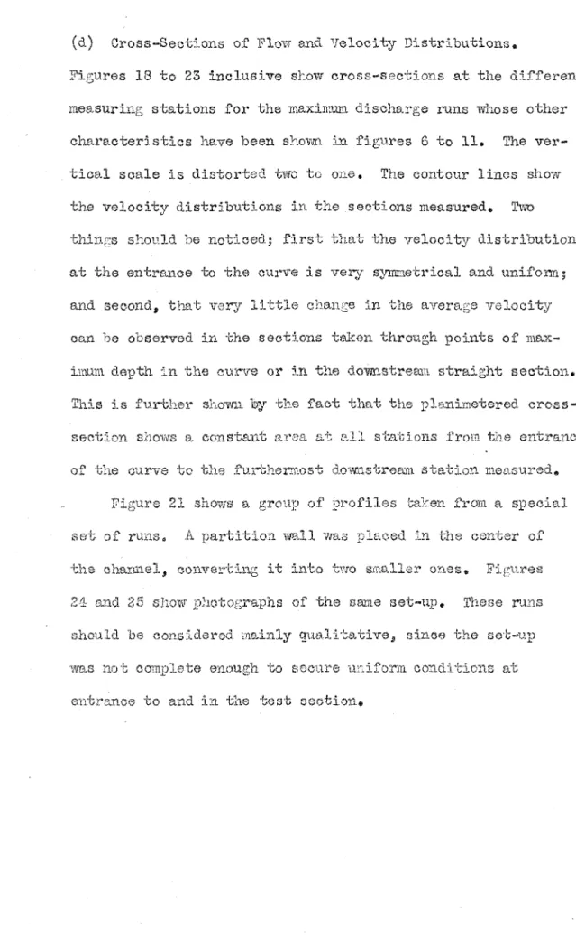
(d) Cross-Sections of Flow anct Velocity Distributions.

Figures 18 to 23 inclusive show cross-sections at the different

m.ea.surin1:; stations for the maximum. discharge runs whose other

characterj sties have been sho11v.n in figures 6 to 11. The

ver-tical scale i.s distorted two to or:.e. The contour lines show

the velocity distributions in the sections measured. Two

thin2:s shoPld be noticed; f:irst that the velocity distribution

at the entrance to the curve is very symmetrical and unifonn; and second, that very little change in the averaf:;e velocity

can be observed in -the sections taken through points of

m.a.x-im.um depth in the curve or in the downstream straight section.

This is further shovr.i by the fact that the plf~nimeterecl

cross-seci;ion sho1Ns a constarrt: r;.1,:rea a~.: all si.K.:'"l.tions :rrorn. t:i1e entrance

Figure 21 shows a group of' profiles ta.ken from a special

set of runs. A partition ·wall was placed in the center of

21 a"l'.ld 25 slwv.r pl-1otot;raphs of the mtme set-up. These runs

should be considered mF.J..inly qualitative,, since the sec-up

·wees nol; complete enough to secure uLiform concl:i.·'cions t'l.t

Q+l5oc

10

o,.,,39Bl

0+4772

~··

Q-+4911

z

.'0

U'b

0+55'"

O+~o''°

RUN 10 CROSS SECTIONS

AND

VELOCITY DISTRIBUTION

R 0 20 n.

s

~ .0995

Q 0 _{192 CF 5.} b ~ I FT

-Q+,398_z

"'

0+44 8r

Figu.re 18

O-r4i"1

0+56°0

:td=:-J

0+6700 RUN 13

CROSS SECTIONS

ANO

VELOCITY DISTRIBUTION

R" IV F'T.

,, " .0997 Q " 2.0~7 C.F. S.

b • I FT.

.. 1"==;$

I ..

~,11

"W

10~

00 I:!>•- - ,'":>

QT42st

0+45"'

0+67"

I

'°ct:J

:D~

0+74"

RUN 19c CROSS SECTIONS

ANO

VELOCITY DISTRIBUTION R = 40f'T

s = .0997

Q = 1.9e5 c.r.s.

b =I FT

0+15°0

Q-1-398Z

Q+44"'

J::='-j

0•")41!?

Figure 19

0 '608_~

30

00--:--:-;-:---r---J

0+71"'

RUN 26 CROSS SECTIONS

ANO

VELOCITY DISTRIBUTION

R = 40 f'T.

s

= .0995 Q = 1983 CFS.

b = I FT

~---·---:~~

0+15°0

'0_{-J-77-77,--~,..J-T-,-,;-,--.,--,,--j}

oolL~JI

0+39el

30

'°

00

:-:--:;--+--_J

0+44ez

L1

0+4811

0+51~

Q+54.'H

0+1.._·-RUN 28 CROSS SECTIONS

AND

VELOCITY DISTRIBUTION Ru 40 FT

s

= .0345 Q = 1973 C.f5.

b ~ I FT

:.klli~

0+15°0

'°~

~=

Q+39!.Z

..

Q+4182

0+43at

Fie;ure 20

l

Q..-478 ' 0+51112 0+555 "

RUN .32 CROSS SECTIONS

AND

VELOCITY DISTRIBUTION

R= 20FT. 5 = 0342

Q = 1.976 C.F S. b = I FT.

""'

0+4240 0+44., 00--<---+---~ 0•46"' JO 00·-<---+---~ 0+47"1 0+63"'

RUN 39 CROSS SECTIONS

AND

VELOCITY DISTRIBUTION R~ IOFT.

s

= 0343 Q = 1.985 C.F'. 5. b ~ I FT.

Figure 21

.•O

00'-'----+--...L---+---'

Q•. 492

'°

Q•.790

.30 20

RUN ISb

STA 0+42'1

RUN 18a

STA 0+42"7

00--L--...j.--...L----t---~

Q•l.960 RUN 18c

STA 0•43"

oo.~---1---~--.,....-~

(" 1025

Q•l.478

Q' 1985

RUN 35 5TA 0+46~

RUN 37 STA. 0+41"'

RUN 36

STA 0+-41'"1

CROSS SECTIONS OF FLOW OUTSIDE R

INSIDE R

WIDTH b

-10.2.5 FT

9.75 FT

0.50 FT

~~

-oo....L--₀-,---4-4---~ ~H

'°

10

oo~---+---'-0+42. e'2.

30 20

00 0+45132.

40 ,o 20 ,0 oo-'---1---__!_ 0•.52" 00 30 20 10 00 20

Ni

0+53 9

~

I

0+5523

0+5817

RUN 52

CROS.S SECTIONS

R 0 _{10 FT.}

S=.0159

Q = 2.32 c.r. s.

b= I FT

Figure 22

00

0•398_z

30 20 10 00 0+43!1'2. 30 20 10 0+4982 0+538Z

0+55 .,~

I

0+571

:;

~

0+59°0

RUN 57

CROSS SECTIONS

R= 20 FT 5= .0155

Q = 2 31 C.F 5.

b= I FT

fl'>

---·~-.)() 10

-w-

10-0+39 '" 0+4682

30 30

20

10 10

00 00

0+413

/j 0+.528?.

30 30

20 20

10 10

00 00

0+44 82 0 ... 5750

RUN 71

CR055 SECTION R0 _{40 FT}

20

5°0155

10 Q0 242 C.F.5.

b0 IFT

00

0+458

-I?.ESUl1TS

T

, L .

Three relations 1•rere obtained in

of flow.,

can be

to

determine of the water surface the walls of a curved channel. Tl1e first two$

on the

of constant is exact

ob-of constant Table 2

the values obtained with these three

as the measured results of 1Nhich we saw

under C. The runs in the were

progre:rn.s

26

the the

TA."BLE 2.

Run _{Station Slope}

I

_Central ~ed Constant Constant

No. Radius Angle Depth Energy Velocity

Discbar~e E> d d(equ.'7) d(equ.S) d(equ. l.Z)

radians feet fee>t feet feet

3 39.82 .0995 0 .150 .150 .150 .150

40.82 20' .05 .205 .201 .203 .198

41.82 1.988 .10 • 25~S .257 .258 .252

42.82 .15 .310 .321 .318 .313

43.65 .191 .349 _{~ ~ ~}

43.82 .20 .363

44.82 .25 .419

45.82 .30 _~

11 39.82 .0995 0 .11~ .111 .111 .111

40.67 101

.085 0190 .183 .183 .176

41.67 1.380 .185 .288 .293 .289 .278

42.67 .285 .392 .429 .417 .399

42.96 .314 .411 .470 .458 .445

.

43.67 .385 .485

44.67 .485 .528

15 39.82 .0995 0 .091 .091 .091 .091

40.67 101

.085 .143 .149 .148 .148

41.67 1.015 .185 .231 .236 .233 .23;:s

42.67 .285 .321 .346 .337 .334

42.93 .311 .350 _~ .372 _~

43.67 .385 .407

44.67 .485 .412

26 39.82 .0995 0 .146 .146 .146 .146

40.82 401

.025 .170 .171 .171 c .170

41.82 l.983 .050 .185 .196 .198 .195

42.82 .075 .216 .223 .223 .222

43.82 .100 .267 .254 .253 .252

44.10 .107 .274 .d§g .263 .260

I

44.82 .125 .:1.§.Q

28 39.82 .0345 0 .200 .200 .200 .200

40.82 401

.025 .207 .221 .218 .219

41.82 l.973 .050 .227 .244 .240 .240

42.82 .075 .257 .266 .263 .261

43.18 .084 .268 _~ .272 .270

53

TABLE 2 (cont.)

Run Station Slope

l

Central Measured Constant Constant

No. Ra.di us lulgle Depth Energy Velocity

Discharge

e

d d(equ.7) d(equ.S) d(equ.12) radians feet feet feet feet

29 39.82 .0345 0 .164 .164 .164 .164

40.82 40' .025 .173 .182 .177 .179

41.82 1.50 .050 .189 .201 .199 .196

42.82 .075 .215 .221 .218 .213

43.28 .086 .225 .229 _~ .223

43.82 .100 _~

32 39.82 .0345 0 .202 .202 .202 .202

40.82 20' .05 .226 .245 .244 .241

41.82 lo976 .10 .285 .293 .290 .284

42.74 .146 .320 _~ .335 .325

42.82 .15 .323

43.82 .20 .329

39 39.82 .0345 0 .212 .212 .212 .212

40.67 101

.085 .277 .290 .286 .278

41.67 l.980 .185 .365 .392 .382 . 366

42.15 .233 .393 .444

_.:.ill

_..:.fil

42.67 .285 .426

43.67 .385 .429

55 39.82 .0145 0 .284 .284 .284 .284

40.82 101

.10 .351 .372 .366 .353

41.63 2.145 .181 .388 .:..1§.Q .443 .410

41.82 .200 .394

42.37 .255 .415

62 39.82 .0145 0 .273 .273 .273 .273

40.82 201

.05 .301 .313 .310 .304

41.79 1.995 .098 .314 .355

_.d12

.337

41.82 .100 .318

vdll be seen that the measured and the calculated values of depth are in very e;ood agreement. The three equations give very similar results. Hmvever equation 12 (constant velocity) appears to give values consistently closer to the observed points than do equations 7 and 8. Equations 7 and 8 differ hardly at all from each other 'vithin the range of practical applications. On the basis of simplicity and of closeness of agreement equation 12 is to be reco!!l:r'lendecl.

All three equations are applicable also to the profile along the inside wa.11 and in this case give the fall. For example, when used f'or the inside wall profile equation 12 becomes

(12a)

cl

=

T

v.i . _sin

a(

f-'., -

a

e)

9 has the negative sign lbiemrnse the wall i.s turning a:way from the flow.

Table 3 presents a. comparison of the values of the maxima calculated from the same three equations and the e:A.-perimental values. All of' the runs :made with simple curves are presented

in this table. It will be noted that in several cases there are