Optimal shunt capacitor allocation and sizing using harmony search algorithm for power loss minimization in radial distribution networks

Full Length Research Article

OPTIMAL SHUNT CAPACITOR ALLOCATION AND SIZING USING HARMONY SEARCH ALGORITHM

FOR POWER LOSS MINIMIZATION IN RADIAL DISTRIBUTION NETWORKS

*1

_{Muthukumar, K.}

_{Dr. Jayalalitha, S.}

_{Dr. Ramasamy, M. and}

_{Haricharan Cherukuri, S.}

1_{Assistant Professor / EEE / SEEE, SASTRA University, Tirumalaisamudram Thanjavur, Tamilnadu, India} 2_{Associate Dean / EIE / SEEE, SASTRA University, Tirumalaisamudram Thanjavur, Tamilnadu, India}

3_{Professor / EEE, Annamalai University, Chidambaram, Tamilnadu, India} 4_{PG scholar, SASTRA University, Tirumalaisamudram Thanjavur, Tamilnadu, India}

ARTICLE INFO ABSTRACT

This study aims to minimize the power loss in radial distribution networks which is realized by injecting reactive power with the aid of shunt capacitors installation at appropriate locations with optimal sizing. A population based meta-heuristic search algorithm namely Harmony search optimization algorithm is utilized for finding out the optimal rating of shunt capacitors to be placed in the radial distribution networks. A Backward / Forward sweep based iterative power flow technique is adopted to compute the load flow solution. The estimation of voltage stability index value of each bus in the proposed radial distribution systems helps to find the optimal locations of shunt capacitor to be placed for reactive power support and to achieve the loss minimization. The robustness of the proposed methodology for optimal shunt capacitor sizing has been tested on 22 and 119 node test systems. Simulation results reveal that the proposed optimization approach is more efficient in finding optimal solution.

Copyright © 2014 Muthukumar et al. This is an open access article distributed under the Creative Commons Attribution License, which permits unrestricted use, distribution, and reproduction in any medium, provided the original work is properly cited.

INTRODUCTION

In the distribution networks, the far end customers will be directly affected by low voltage problems due to more loss along the feeder lines and its sub laterals. The power loss associated with the Radial Distribution System (RDS) is more when compared with the transmission network due to its interest high R/X ratios, unbalanced loadings, untransposed feeder lines. To achieve the loss reduction in the distribution networks, various methods are proposed in the literature such as optimal conductor sizing, System Reconfiguration, shunt capacitor placement at appropriate locations with optimal ratings. Shunt capacitor installation at/or near to the loads improves the system efficiency if capacitors are to be optimally sized and located at appropriate locations. There is a chance of bus voltages exceeds the prescribed limit as a consequence of improper size of capacitor located at wrong places. An efficient distribution system load flow technique is needed for finding out the power losses as well as the node voltages and

*Corresponding author:Muthukumar, K. Assistant Professor / EEE / SEEE, SASTRA University, Tirumalaisamudram Thanjavur, Tamilnadu, India.

the branch currents in the system at specified loading conditions. A load flow approach for solving the distribution system power flow problems which uses Triangular factorization known as implicit ZBUS Gaussian method was proposed by Chen et al. in (1991). Shirmohammadi (1988) proposed a method for solving weakly meshed distribution systems by using basic Kirchhoff’s laws and the proposed methodology can be applied for balanced as well as unbalanced networks. An approach for solving the power flow solution in radial distribution systems by using the Backward and Forward sweep has been proposed by Thukaram (1999). Das et al. (1995) suggested a methodology for power flow solution using the Backward & Forward approach. A quadratic equation approach for finding out the weaker nodes in the distribution networks has been proposed in (Gozel et al., 2008) by Gozel. Various voltage stability indices available to find the weak nodes in the distribution system has been compared in (2009) by Eminoglu. A Voltage stability index suitable to identify the weak nodes in the RDS has been proposed by Chakravorty Das in (2001) considering the composite loading nature of the radial distribution systems. Sirjani et al. (2010) proposed the HSA based approach for capacitor placement (CP) for loss reduction. A network topology based power flow

ISSN:

2230-9926

Vol. 4, Issue, 3, pp. 537-545, March,2014

DEVELOPMENT RESEARCH

Article History:

Received 08th January, 2014 Received in revised form 11th February, 2014 Accepted 15th

February, 2014 Published online 14th

March, 2014

Key words:

technique is proposed by Teng in (2000). Geem et al. in (2001) (Lee and Geem 2005) proposed new meta heuristic optimization technique namely Harmony search Algorithm (HSA) for solving the combinatorial optimization problems. HSA based optimal sizing of shunt capacitor has been suggested in (Muthukumar and Jayalalitha 2012; Muthukumar Jayalalitha and 2013) to reduce the cost of power loss along

with installation cost of shunt capacitors. Ramalinga Raju

et al. (Ramalinga Raju et al., 2012) proposed a direct search algorithm for shunt capacitor placement in RDS.

Problem Formulation

In distribution network, power loss is a major concern which affects the consumers directly and one efficient way to reduce the power loss in the primary feeder lines is by installing the shunt capacitors which injects the reactive powers partially near to the consumer loads. The objective function of the proposed study is to curtail the power loss by reducing the reactive part of the branch currents and it can be stated mathematically as in Eq.(1&2)

Minimize

Ploss = Ploss = |I | . R (1)

k = 1, 2, 3… nb

In a radial distribution network with “nb” number of branch sections, the total power loss can be stated as, loss

Ploss = (|I | R + |I | X ) (2)

k = 1, 2, 3… nb

The total power loss is the summation of power losses associated with the real and reactive part of branch current magnitude in all the branches of the RDS as shown in Eq. (2). The proposed approach aims to reduce the total real power loss of the proposed test systems by reducing the reactive part of branch currents by partially injecting the reactive power using the shunt capacitors installation at appropriate locations with proper sizes. The following inequality constraints are to be satisfied for the proposed objective function minimization.

Bus voltage magnitudes

The bus voltage magnitude at each bus should lie in between the specified tolerance limits. ±5 % of the nominal bus voltage as in Eq.(3).

Vkmin < Vk < Vkmax k=1,2….n (3)

Thermal loading limit of the feeder lines

The current through each branch of the feeder lines should be less than their maximum thermal limit

Ibk < Ibkmax k =1,2….nb (4)

Rating and total number of shunt capacitors

The multiple integers of the smallest size of standard capacitor available in the market with discrete sizes is one of the

constraints and the total reactive power supplied by the installed capacitors should not exceeds the total reactive power demand of the RDS

Qck ≤ P Qc, where P=1,2…,nc (5)

∑ ≤

(6)

Power Flow Solution

The application of Newton Raphson or Gauss-Seidel methods for power flow solutions is not suitable for radial distribution system due to its higher R/X ratio and unbalanced loadings nature. To get the power flow solutions in RDS, various types of distribution load flow techniques were proposed and most of the methods are based on Kirchhoff’s current law (KCL) and voltage law (KVL). Backward/Forward sweep based technique BPS is one of the efficient and most effective method used to get the power flow solution of RDS, which computes currents at all nodes from the end node towards the source node in the backward sweep mode and respective bus voltages are computed from source nodes towards the end notes in the forward sweep mode (Teng 2000).

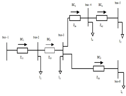
Fig 1. Sample radial distribution network

For the sample six bus RDS is shown in Fig.1, The current in each branches and bus voltages are calculated by using BFS based iterative technique. Equivalent current injected at kth node is computed as in Eq.(7)

Ik = ∗∗ where k = 2,3,….,n (7)

where Sk* is the conjugate of complex power of kth node, Vk* is the conjugate of kth node voltage and “n” represents the total nodes available in the given radial network.

Formulation of BIBC matrix

After the computation of injected node currents, the corresponding branch currents (BC) are calculated as,

where I2 ,I3….I6 are the equivalent current injection of respective nodes.

The incidence matrix which relates the injected node current to branch current (BIBC) can be formulated as in Eq (8).The (BIBC) matrix dimension is nb x n, if the distribution system contains nb number of branches with n nodes.

⎣ ⎢ ⎢ ⎢ ⎡ ⎦ ⎥ ⎥ ⎥ ⎤ = ⎣ ⎢ ⎢ ⎢

⎡1 1 1 1 1_{0 1 1 1 1}

0 0 1 1 0 0 0 0 1 0

0 0 0 0 1⎦

⎥ ⎥ ⎥ ⎤ ⎣ ⎢ ⎢ ⎢ ⎡ ⎦ ⎥ ⎥ ⎥ ⎤ (8)

The above branch current matrix can be represented in a compact form as,

[ ]=[ ][ ]

Formulation of BCBV Matrix

The voltage of each node can be calculated from substation bus towards the terminal node after calculating the current injection by each load and branch currents beginning from the end node towards the root node. The incidence matrix which relates the branch current and bus voltage can be formulated as in Eq. (9)

(BCBV)=(BIBC)T_{(ZD) (9)}

Where “T” represents the transpose of (BIBC) matrix, and (ZD) is the impedance matrix with impedance of each branch as the diagonal element as shown in Eq. (10).

(ZD)=

0 0 0 0

0 0 0 0

0 0 0 0

0 0 0 0

0 0 0 0

(10)

Where Z1, Z2, Z3, Z4, Z5 are the respective branch impedances of the sample system. The final form of (BCBV) matrix can be represented as in Eq. (11).

(BCBV)=

⎣ ⎢ ⎢ ⎢

⎡ 0 0₀ 0₀ 0₀

0 0

0

0 0 ⎦

⎥ ⎥ ⎥ ⎤

(11)

Then the bus voltages can be computed by using the (BCBV) matrix and branch current matrix (BC) as in Eq. (12)

⎣ ⎢ ⎢ ⎢ ⎡ ⎦ ⎥ ⎥ ⎥ ⎤ = ⎣ ⎢ ⎢ ⎢ ⎡ ⎦ ⎥ ⎥ ⎥ ⎤ -⎣ ⎢ ⎢ ⎢

⎡ 0 0₀ 0₀ 0₀

0 0

0

0 0 ⎦

⎥ ⎥ ⎥ ⎤ ⎣ ⎢ ⎢ ⎢ ⎡ ⎦ ⎥ ⎥ ⎥ ⎤ (12)

Where V1 is slack bus voltage and it is taken as 1 p.u and the remaining bus voltages are assumed as 1.0 p.u for the first iteration in backward sweep mode for calculation of load

currents and the new value of bus voltages are updated as the iteration process progresses in forward sweep mode using Eq (12). This backward and forward sweep based iterative process is repeated until the convergence is reached.

Voltage Stability Index

The stability of the radial distribution network can be found by computing the voltage stability index (VSI) of each node. The stability index value near to 1.0 will be the indication of a stable system (Chakravorty and Das 2001). The candidate node with lower value of index is identified as the sensitive node and more chance for voltage collapse among all nodes and it is the well suited place for installation of shunt capacitors.

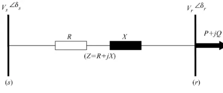
Fig 2. Branch of Radial Distribution Network

Where “r” indicates the succeeding node, Vs is preceding node voltage and Vr is the succeeding node voltage. P and Q represent the active, reactive power loads which are lumped at the succeeding node r. X and R are the effective reactance and resistance of the bus section. Using Eq.(13) the VSI of succeeding node r can be calculated as,

VSI(r) = {|Vs| 4 – 4. 0 |Vs|2 {P R + QX} – 4.0

{PX - QR}2 } (13)

For stable operation of the radial distribution system with “n” number of nodes,

VSI (r) ≥ 0, where r = 2, 3... n.

Harmony Search Algorithm

HSA has been proposed by Geem, Kim and Loganathan

Step-1: Parameters initialization of HSA algorithm. Step-2: Initialize of Harmony Memory Vector (HMV) Step-3: Improvisation process of the new Harmony Memory vector.

Step-4: Updating the Harmony vector values.

Step-5: Repeat step 3 & 4 until the termination criteria has been mot.

Step- 1 Initialize the parameters of HSA

HSA parameters are initialized by choosing the suitable value for HM size. It is used to decide the number of decision vectors and in the HM, a group of decision variables are stored. The Harmony Memory Consideration Rate (HMCR) and Pitch Adjusting Rate (PAR) are utilized to get best solution vector to be stored in HM.

Step-2 HMV initialization

In Harmony Memory Vector (HMV), solution vectors are randomly generated within their lower and upper bound limits are utilized to form the HMS matrix

Step- 3. Improvisation of Harmony Memory (HMV)

The following three measures are adopted to improve the New Harmony vector value (10). The first one is Memory Consideration, second one is Pitch Adjustment and third one is Random Selection. The variable values of HM vector x2’,x3’,…xN’ are selected randomly. The HMCR value is chosen within 0 and 1, and it is the rate of selecting one decision variable value from the previously stored values in the Harmony Memor. (1- HMCR) is the rate of randomly choosing each decision variable value from the specified bound of values as in Eq. (14),

if (rand ( ) < HMCR)

xi← xi ∈ {xi1 , xi2 , ..., xi HMS} else

xi ← xi ∈ Xi

end (14)

rand ( ) represents the uniform random number lies within 0 to 1 and “Xi” is the possible range of values for each decision variable (xi’). if HMCR value chosen as 0.9, then the HS algorithm will select the decision variable from the values stored in the Harmony Memory with the probability of 90 %, (or) from the possible range lies between (100-90) % probabilities (Muthukumar and Jayalalitha 2012). Each element from the memory consideration is to be pitch adjusted as,

If (rand ( ) < Pitch adjustment rate xi’=xi’± bw*rand ( )

else

xi’=xi’ (15)

“bw” represents a step size or random distance bandwidth.

Step-4. Updating Harmony Memory Vector (HMV). A new modified and improved harmony vector values and its best fitness function values computed in step 3 are added in HM by replacing the existing worst harmony vector. Otherwise, the new generated vector value is discarded. Step- 5: Step 3 and Step 4 are repetitive until the termination condition is reached.

RESULTS AND DISCUSSIONS

Methodology for identification of optimal location

A steady state voltage stability index for RDS to identify most sensitive buses that leads to voltage collapse are computed by using Eq. (13) to ensure the right place for capacitor installation. The node with lower value of VSI is considered as higher priority candidate node for placement of shunt capacitor. The VSI of each node in the proposed test systems has to be computed to find out the weak nodes. The bus voltage magnitudes, line flows and corresponding line loss are computed using the BFS based load flow technique. In HSA algorithm begins with random generation of the solution vectors without violating the constraints associated with the proposed objective function (i.e. random capacitor selection within the commercially available capacitor sizes). The HM matrix is filled with random solution vectors and its corresponding objective functions (real power loss) can be represented as (Muthukumar and Jayalalitha 2012),

HMS= (Qci, Qc2, … , Qcn)

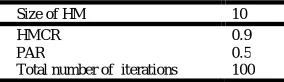
In the subsequent iterative steps of HS algorithm, the stored vectors with its fitness values in the HM matrix are improved by eliminating the worst solution vectors by the improvisation steps such as memory consideration, Pitch adjustment rate, random selection process until the stopping criterion is reached. The proposed HSA algorithm is applied successfully for optimal sizing of capacitors on 22 node and 119 node test systems with real power loss minimization. The algorithm is implemented in Matlab 7.7.0 on a system with Intel core i5 processor. The selection of HSA parameters plays a vital role for the speed of convergence towards the global solution (Muthukumar and Jayalalitha 2013) The HSA tuning parameters are chosen for the proposed test systems after multiple test runs to demonstrate the algorithm effectiveness is shown in Table 1.

Table 1. HSA Parameters

Size of HM 10

HMCR 0.9

PAR 0.5

Total number of iterations 100

Example 1: Practical 22- Node radial distribution system:

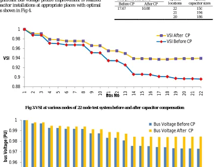
Fig.3 and it is pragmatic that the enhancement in the bus stability indices after capacitive compensation. It is observed that a significant bus voltage profile improvement is realized after capacitor installations at appropriate places with optimal ratings as shown in Fig 4.

Table 2. Simulation results of 22 Node test system

Real power loss (KW) Optimal locations

Optimal capacitor sizes Before CP After CP

17.67 10.88 22 150 21 194 20 186

Fig 3.VSI at various nodes of 22 node test system before and after capacitor compensation

Fig 4. Bus voltage Magnitude of 119 node test system before and after capacitor compensation

Fig 5. VSI at va rious nodes of 119 node test system before and after capacitor compensation 0.88

0.9 0.92 0.94 0.96 0.98 1

1 2 3 4 5 6 7 8 9 _{10 11 12 13 14 15 16 17 18 19 20 21 22}

VSI

Bus No

VSI After CP VSI Before CP

0.95 0.96 0.97 0.98 0.99 1

1 2 3 4 5 6 7 8 9 _{10 11 12 13 14 15 16 17 18 19 20 21 22}

b

u

s

V

o

lt

a

ge

(PU

)

Bus No

Bus Voltage Before CP Bus Voltage After CP

0.3 0.4 0.5 0.6 0.7 0.8 0.9 1 1.1

1 3 5 7 9 _{11 13 15 17 19 21 23 25 27 29 31 33 35 37 39 41 43 45 47 49 51 53 55 57 59 61 63 65 67 69 71 73 75 77 79 81 83 85 87 89 91 93 95 97 99}

101 103 105 107 109 111 113 115 117 V S I

Bus No

VSI Before CP

Example-2: 119 bus test system

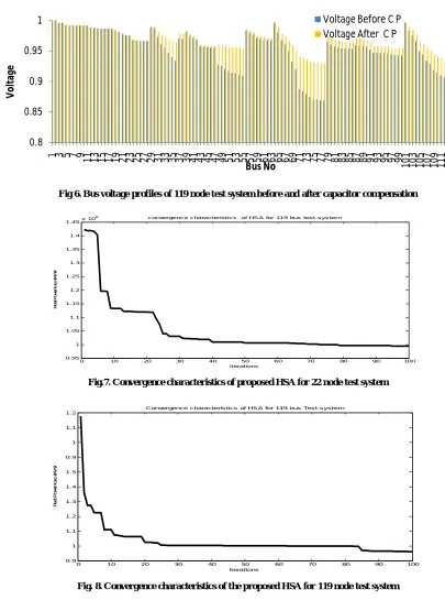
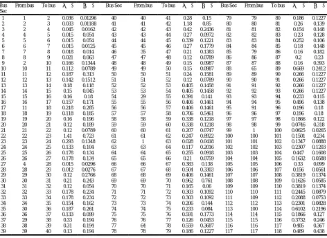
To investigate the efficiency of the proposed methodology in a large scale radial distribution network, it was implemented on 119 node test system contains 117 branches. The active and reactive load demand of the test system is 22709.72KW and 17041.07 KVAr respectively. The system is operated with the nominal bus voltage of 11 KV, 100 MVA base. The nodes of 119 bus test system have been renumbered as shown in Fig 9 and to preserve the radiality, the tie switches in the original test system (Dong Zhang et al., 2007) have been removed. The load and line data is given in Table A1 and Table A2 in Appendix A. The BFS

based power flow technique is utilized to find out the bus voltage magnitude, line flows and total real power loss at nominal load condition and the real power loss obtained before capacitor placement is 1291 KW. The VSI values of all nodes in the proposed test network before and after capacitor placement are estimated using Eq.(13) and the corresponding VSI values are plotted as shown in Fig. 5. Based on the computed VSI values 21 nodes are identified as the sensitive nodes for capacitor placement and the amount of reactive power injection by the shunt capacitors is optimized by the HSA algorithm. The simulation results of optimal capacitor sizes and its corresponding locations, total system real power

Fig 6. Bus voltage profiles of 119 node test system before and after capacitor compensation

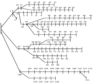
Fig.7. Convergence characteristics of proposed HSA for 22 node test system

Fig. 8. Convergence characteristics of the proposed HSA for 119 node test system 0.8

0.85 0.9 0.95 1

1 3 5 7 9 11 13 15 17 19 21 23 25 27 29 31 33 35 37 39 41 43 45 47 49 51 53 55 57 59 61 63 65 67 69 71 73 75 77 79 81 83 85 87 89 91 93 95 97 99 _{101 103 105 107 109 111 113 115 117 119}

V

o

lt

a

ge

Bus No

Voltage Before C P Voltage After C P

0 10 20 30 40 50 60 70 80 90 100

0.95 1 1.05 1. 1 1.15 1. 2 1.25 1. 3 1.35 1. 4

1.45x 10

6

it erat ions

R

e

a

l

P

o

w

e

r

lo

s

s

(

K

W

)

c onvergenc e c haract erist ic s of HSA for 119 bus test s ys tem

0 10 20 30 40 50 60 70 80 90 100

0.9 1 1.1 1.2 1.3 1.4 1.5 0.9 1 1.1 1.2

iterations

R

e

a

l

P

o

w

e

r

lo

s

s

(

K

W

)

loss before and after capacitor placements are summarized in Table 3. The bus voltage profile before and after capacitive compensation is shown in Fig.6. Simulation results reveal the effectiveness of proposed HSA algorithm to find the optimal capacitor sizes to achieve the power loss minimization from 1291 KW to 926.1KW (loss reduction of 28.26 %)

Table 3. Simulation results of 119 Node test system

Convergence characteristics of HSA algorithm

The robustness of the HSA algorithm is tested by tuning the control parameters. Solution (real power loss) of the proposed test systems is obtained by 30 independent runs of the HSA

algorithm with different random population. The exploration and exploitation ability of the HSA algorithm towards the optimum solution for the proposed test systems are shown in Fig 7and Fig 8.

Nomenclature

nb :Total number of branches in m node RDS. Ploss : Total sum of real power loss in KW |I_bk | : Magnitude of k th branch current Rk : kth .branch conductor resistance in Ω X k : kth.branch conductor reactance in Ω nc :Total number of capacitors to be installed nb : Number of branches in the RDS

n : Number of nodes in RDS Ibrk : kth branch current Vk : kth Bus voltage

Vk min : Lower bound of kth node voltage Vk max : Upper bound of kth node voltage [BIBC] : Incidence matrix relates the node current injection to branch currents

[BCBV] : Incidence matrix relates the branch currents to node voltages

[BC] : Branch current vector [Z] : Impedance Matrix

Qc : Minimum Ratings of available capacitors. Qd :Total KVAr demand of load in RDS Ibkmax : Maximum allowable k th branch current [I] : Bus current injection vector

T : Matrix transpose

Conclusion

In this study, optimal capacitor allocation and sizing problem is solved by implementing Harmony Search Algorithm to

Real Power loss before CP 1291 KW Real Power loss after CP 926.1KW

S.No Optimal Locations Optimal Capacitor sizes(KVAr) 1

2 3 4 5 6 7 8 9 10 11 12 13 14 15 16 17 18 19 20 21

79 77 76 75 74 73 72 113 56 115 54 53 111 52 112 51 71 110 50 70 49

714 170 192 509 272 432 386 974 375 493 377 425 641 753 793 349 513 281 165 626 488

achieve the significant reduction in power loss along with the benefits such as improvement in bus voltage magnitude and voltage stability index of the proposed test systems. The convergence ability of the HSA towards the optimal solution has been demonstrated in large scale radial distribution system like 119 bus test system indicates its robustness to reach the optimal solution. The optimal location for capacitor installation is identified based on the VSI value of each node of the proposed 22 bus and 119 bus test systems and HSA has been utilized to find the optimal shunt capacitor ratings. It is concluded that the proposed HS algorithm is well suited to solve the nonlinear integer optimization problems.

REFERENCES

Chakravorty M., D. Das, “Voltage stability analysis of radial distribution networks,” International journal of Electrical power and energy system, vol.23, pp 129-135, 2001. Chen T.H., M.-S. Chen, K.-J. Hwang, P. Kotas, and E. A.

Chebli, “Distribution system power flow analysis - A rigid approach,” IEEE Trans. Power Delivery, vol. 6, pp. 1146– 1152, July 1991.

Das D., D. P. Kothari, and A. Kalam, “Simple and efficient method for load flow solution of radial distribution networks,” Electrical Power & Energy Systems, vol. 17. N0.5, pp 335-346, 1995.

Dong Zhang, Zhengcai Fu, Liuchun Zhang, “An improved TS algorithm for loss minimum reconfiguration in large scale distribution systems”, Electrical power system Research, Vol 77,PP 685-694, 2007

Eminoglu U. and M.H.Hocaoglu, “A Network topology based voltage stability index for radial distribution networks”, International Journal of Electrical Power and Energy Systems, vol.29, no.2, pp 131-143, 2009

Geem, Z.W., J.H.Kim and G.V.Loganathan, “A new heuristic optimization algorithm: Harmony search”, Simulation, vol 76:no.2. PP:60-68,2001

Gozel T., U. Eminoglu, M.H.Hocaoglu, “A tool for voltage stability and optimization (VS&OP) in radial Distribution systems using Matlab graphical interface (GUI)”, Simulation Modeling practice and theory, vol.16,no.5, May2008, pp 505-518.

K.Muthukumar, Dr.S.Jayalalitha, “Harmony Search Approach for Optimal Capacitor Placement and Sizing in Unbalanced Distribution Systems With Harmonics Consideration”, IEEE International Conference on Advances in Engineering, Science and Management, ICAESM-2012, pp. 393-398, 30, 31 March 2012.

Lee, K. and Z.Geem,“A new meta heuristic algorithm for continuous engineering optimization: Harmony Search theory and practice”, Comput. Methods Applied Mechanics Eng 194:3902-3933, 2005.

Muthukumar K., Dr.S.Jayalalitha, “Optimal Reactive Power Compensation by Shunt Capacitor Sizing Using Harmony Search Algorithm in Unbalanced Radial Distribution System for Power loss Minimization”, International journal of Electrical Engineering and informatics, Volume 5 ,No: 4,PP 474-491, December 2013.

Ramalinga Raju M., K.V.S. Ramachandra Murthy and K.Ravindra, “Direct search algorithm for capacitive compensation in radial distribution systems”, International journal of power & Energy Systems, vol 42, PP 24-30, 2012

Shirmohammadi D., H. W. Hong, A. Semlyen, and G. X. Luo, “A compensation-based power flow method for weakly meshed distribution and transmission networks,” IEEE Trans. Power Syst., vol. 3, pp.753- 762, May 1988. Sirjani R., A. Mohamed, H.Shareef, “Optimal capacitor

placement in a radial distribution system using Harmony search algorithm”, Journal of applied sciences 10(23), PP: 2998-3006, 2010.

Teng, J. H., “Network-topology-based three-phase load flow for distribution systems”, Proc. Natl. Sci. Counc. ROC (A), Vol.24, no.4, PP. 259-264, 2000.

Thukaram, D., Wijekoon Banda, H. M. and Jerome, J., “A robust three phase power flow algorithm for radial Distribution systems,” Electric Power Systems Research, vol.50, no.3, pp. 227-236, 1999.

Appendix- A

Table: A1. 119 –Bus Network Load Data

Bus PL(KW) QL(KVAr) Bus.No PL(KW) QL(KVAr) Bus.No PL(KW) QL(KVAr)

1 0 0 40 393.05 342.6 79 294.55 162.47

2 133.84 101.14 41 326.74 278.56 80 485.57 437.92

3 1 11.292 42 536.26 240.24 81 243.53 183.03

4 34.315 21.845 43 76.247 66.562 82 243.53 183.03

5 73.016 63.602 44 53.52 39.76 83 134.25 119.29

6 144.2 68.604 45 40.328 31.964 84 22.71 27.96

7 104.47 61.725 46 39.653 20.758 85 49.513 26.515

8 28.547 11.503 47 66.195 42.361 86 383.78 257.16

9 87.56 51.073 48 73.904 51.653 87 49.64 20.6

10 198.2 106.77 49 114.77 57.965 88 22.473 11.806

11 146.8 75.995 50 918.37 1205.1 89 62.93 42.96

12 26.04 18.687 51 210.3 146.66 90 30.67 34.93

13 52.1 23.22 52 66.68 56.608 91 62.53 66.79

14 141.9 117.5 53 42.207 40.184 92 114.57 81.748

15 21.87 28.79 54 433.74 283.41 93 81.292 66.526

16 33.37 26.45 55 62.1 26.86 94 31.733 15.96

17 32.43 25.23 56 92.46 88.38 95 33.32 60.48

18 20.234 11.906 57 85.188 55.436 96 531.28 224.85

19 156.94 78.523 58 345.3 332.4 97 507.03 367.42

20 546.29 351.4 59 22.5 16.83 98 26.39 11.7

21 180.31 164.2 60 80.551 49.156 99 45.99 30.392

22 93.167 54.594 61 95.86 90.758 100 100.66 47.572

23 85.18 39.65 62 62.92 47.7 101 456.48 350.3

24 168.1 95.178 63 478.8 463.74 102 522.56 449.29

25 125.11 150.22 64 120.94 52.006 103 408.43 168.46

26 16.03 24.62 65 139.11 100.34 104 141.48 134.25

27 26.03 24.62 66 391.78 193.5 105 104.43 66.024

28 594.56 522.62 67 27.741 26.713 106 96.793 83.647

29 120.62 59.117 68 52.814 25.257 107 493.92 419.34

30 102.38 99.554 69 66.89 38.713 108 225.38 135.88

31 513.4 318.5 70 467.5 395.14 109 509.21 387.21

32 475.25 456.14 71 594.85 239.74 110 188.5 173.46

33 151.43 136.79 72 132.5 84.363 111 918.03 898.55

34 205.38 83.302 73 52.699 22.482 112 305.08 215.37

35 131.6 93.082 74 869.79 614.775 113 54.38 40.97

36 448.4 369.79 75 31.349 29.817 114 211.14 192.9

37 440.52 321.64 76 192.39 122.43 115 67.009 53.336

38 112.54 55.134 77 65.75 45.37 116 162.07 90.321

39 53.963 38.998 78 238.15 223.22 117 48.785 29.156

118 33.9 18.98

Table A2. 119 –Note Network Line Data

Bus Sec

From bus To bus R(Ω) X(Ω) Bus Sec From bus To bus R(Ω) X(Ω) Bus Sec From bus To bus R (Ω) X(Ω)

1 1 2 0.036 0.01296 40 40 41 0.28 0.15 79 79 80 0.186 0.1227

2 2 3 0.033 0.01188 41 41 42 1.18 0.85 80 80 81 0.26 0.139

3 2 4 0.045 0.0162 42 42 43 0.42 0.2436 81 81 82 0.154 0.148

4 4 5 0.015 0.054 43 43 44 0.27 0.0972 82 82 83 0.23 0.128

5 5 6 0.015 0.054 44 44 45 0.339 0.1221 83 83 84 0.252 0.106

6 6 7 0.015 0.0125 45 45 46 0.27 0.1779 84 84 85 0.18 0.148

7 7 8 0.018 0.014 46 35 47 0.21 0.1383 85 79 86 0.16 0.182

8 8 9 0.021 0.063 47 47 48 0.12 0.0789 86 86 87 0.2 0.23

9 2 10 0.166 0.1344 48 48 49 0.15 0.0987 87 87 88 0.16 0.393

10 10 11 0.112 0.0789 49 49 50 0.15 0.0987 88 65 89 0.669 0.2412

11 11 12 0.187 0.313 50 50 51 0.24 0.1581 89 89 90 0.266 0.1227

12 12 13 0.142 0.1512 51 51 52 0.12 0.0789 90 90 91 0.266 0.1227

13 13 14 0.18 0.118 52 52 53 0.405 0.1458 91 91 92 0.266 0.1227

14 14 15 0.15 0.045 53 53 54 0.405 0.1458 92 92 93 0.266 0.1227

15 15 16 0.16 0.18 54 29 55 0.391 0.141 93 93 94 0.233 0.115

16 16 17 0.157 0.171 55 55 56 0.406 0.1461 94 94 95 0.496 0.138

17 11 18 0.218 0.285 56 56 57 0.406 0.1461 95 91 96 0.196 0.18

18 18 19 0.118 0.185 57 57 58 0.706 0.5461 96 96 97 0.196 0.18

19 19 20 0.16 0.196 58 58 59 0.338 0.1218 97 97 98 0.1866 0.122

20 20 21 0.12 0.189 59 59 60 0.338 0.1218 98 98 99 0.0746 0.318

21 21 22 0.12 0.0789 60 60 61 0.207 0.0747 99 1 100 0.0625 0.0265

22 22 23 1.41 0.723 61 61 62 0.247 0.8922 100 100 101 0.1501 0.234

23 23 24 0.293 0.1348 62 1 63 0.028 0.0418 101 101 102 0.1347 0.0888

24 24 25 0.133 0.104 63 63 64 0.117 0.2016 102 102 103 0.2307 0.1203

25 25 26 0.178 0.134 64 64 65 0.255 0.0918 103 103 104 0.447 0.1608

26 26 27 0.178 0.134 65 65 66 0.21 0.0759 104 104 105 0.1632 0.0588

27 4 28 0.015 0.0296 66 66 67 0.383 0.138 105 105 106 0.33 0.099

28 28 29 0.012 0.0276 67 67 68 0.504 0.3303 106 106 107 0.156 0.0561

29 29 30 0.12 0.2766 68 68 69 0.406 0.1461 107 107 108 0.3819 0.1374

30 30 31 0.21 0.243 69 69 70 0.962 0.761 108 108 109 0.1626 0.0585

31 31 32 0.12 0.054 70 70 71 0.165 0.06 109 109 110 0.3819 0.1374

32 32 33 0.178 0.234 71 71 72 0.303 0.1092 110 110 111 0.2445 0.0879

33 33 34 0.178 0.234 72 72 73 0.303 0.1092 111 109 112 0.2088 0.0753

34 34 35 0.154 0.162 73 73 74 0.206 0.144 112 112 113 0.2301 0.0828

35 30 36 0.187 0.261 74 74 75 0.233 0.084 113 100 114 0.6102 0.2196

36 36 37 0.133 0.099 75 75 76 0.591 0.1773 114 114 115 0.1866 0.127

37 29 38 0.33 0.194 76 76 77 0.126 0.0453 115 115 116 0.3732 0.246

38 38 39 0.31 0.194 77 64 78 0.559 0.3687 116 116 117 0.405 0.367

39 39 40 0.13 0.194 78 78 79 0.186 0.1227 117 117 118 0.489 0.438