Direct Numerical Simulation of the Airfoil Segment's Flutter and its Effect on the Aerodynamic Force

Direct Numerical Simulation of the Airfoil Segment’s

Flutter and its Effect on the Aerodynamic Force

Andrei Zelenyy

∗

,

Alexey Bunyakin

Faculty of Mathematics and Computer Sciences, Kuban State University, Krasnodar, 350040, Russian Federation

Copyright c2017 by authors, all rights reserved. Authors agree that this article remains permanently open access under the terms of the Creative Commons Attribution License 4.0 International License

Abstract

This article presents numerical simulation of planar potential flow around an airfoil with possibility of changing its shape. Two-dimensional unsteady flow model with scalar velocity potential, which allows us to calculate pressure distribution along an airfoil from Cauchy-Lagrange integral, is used. For this purpose, an airfoil contour is approximated by a complex cubic spline with possibility of displacement its vertices. This algorithm has been used in the context of fluid-structure interaction and has been applied successfully to determination of stability of an elastic airfoil segment interacting with a flow stream, so-called panel flutter problem. Calculation of external flow is carried out by vortex panel method with Kutta-Joukowski trailing edge condition, which makes mathematical solu-tion unique. Using this method of approximation of an airfoil in combination with the method of discrete vortices provides a semi-analytical solution for complex potential for whole computational domain of air flow. This solution significantly accelerates process of numerical computation of time-averaged aerodynamic force as well as the dynamic stability problem for aeroelastic wing design and temporal evolution of its natural disturbances.

Keywords

Aeroelasticity, Aerodynamic Force, Lift Aug-mentation, Vortex Panel Method, Subsonic Flutter, Limit Cy-cle Oscillations

1

Introduction

Aeroelastic phenomena can occur to many engineering structures. In recent years, beneficial effects of aeroelasticity have received greater attention. For example, promise of new aerospace systems such as uninhabited air vehicles (UAVs) and morphing aircraft will undoubtedly be more fully real-ized by exploiting the benefits of aeroelasticity while miti-gating risks.

Reliable aeroelastic analysis tools are needed to reduce ex-pensive and time consuming experimental tests. In a later development an alternative approach has gained popularity

which is known as “double-lattice”method [1,2] (DLM). The DLM is one of the most powerful tools for linear flutter anal-yses in subsonic regime. In this approach a lifting surface is divided into boxes (panels) and collocation is used for both downwash and pressure. For subsonic flows, numeri-cal methods are in an advanced state of development. Paper by Rodden et al[3] contains an extensive discussion of the numerical techniques.

Roughenet al. [4] have compared results of several theo-retical models with experimental data from a Benchmark Ac-tive Controls Technology (BACT) wing (see also [5]). The BACT wing is a rectangular planform with a NACA 0012 airfoil profile. The model has a trailing edge control sur-face extending from 45 to 75% span. Previously, Schuster et al. [6] had compared results from a Navier-Stokes CFD model (ENS3DAE) to these experimental data. Roughenet al. used an alternative Navier-Stokes CFD model (CFL3D) and a classical potential flow model (doublet-lattice). Cor-relations were made at several subsonic to transonic Mach numbers. As they note:

. . .For the purely subsonic condition(M = 0.65). . . .there is relatively good agreement between the doublet-lattice re-sults, the Navier-Stokes results and the test data. This is not surprising because the flow is entirely subsonic and well be-haved(there is no shock wave and no flow separation). . .

Another valuable correlation among several theoretical re-sults and that of experiment is based upon the experimental work of Davis and Malcolm [7] (for more discussions, see Dowell [8]).

All above mentioned facts are reliable foundation for ap-plying inviscid flow model to computation basic properties of fluid (air) flow.

Our fluid model is based upon Euler (momentum) equa-tion of moequa-tion and does not cause significant difficulties for its numerical solution. Assuming flow is incompressible and irrotational and using the vortex panel method together with Cauchy-Lagrange integral for non-steady flow with proper boundary conditions allows us to relate dynamic pressure to scalar velocity potential.

aeroelastic-ity, first addressed by Fung [9] and Kobayashi [10]. This is a flutter resulting from fluid flow over an elastic plate. Dowell and coworkers [11–14] have done extensive numerical simu-lation of the panel flutter and mechanics of this problem. See also recent research results that have been obtained in the last decade in works of Vedeneevet al.[15–19].

Fluid-structure interaction solution requires that we solve fluid and structural models simultaneously for unknown pres-sure and body motion.

Airfoil profile shape is known to be an important param-eter. This paper demonstrates a new airfoil approximation method with a sharp trailing edge by known control points (airfoil profile frame). This algorithm successfully applied in description of fluid-structure interaction of flow stream over an oscillating elastic segment (section) of an airfoil. Linear discretization of vorticity field and replacement of the air-foil by its approximate coordinates allows us to numerically calculate pressure distribution and scalar velocity potential both for steady and unsteady case. As a result of the linear discretization the problem is reduced to solution of a system of linear algebraic equations in unknown point vortices. To make the system complete an additional restriction is made, so-called Kutta-Joukowski trailing edge condition. This re-striction states, in our case, that the point vortices on trailing edge must be the same magnitude and spinning in opposite directions to satisfy the Kutta condition.

Dividing entire flow field into two simply-connected do-mains enables to find a semi-analytical expressions for com-plex potential in each of these domains. These semi-analytical expressions significantly accelerate computation of basic characteristics of fluid flow, as well as numerical calcu-lation of time-averaged lift force of a wing.

The last chapter of the article is devoted to numerical study of stability of an airfoil which takes into account unsteady motion near oscillating segment. Dynamic system of fluid-structure interaction is described. Obtained results were stud-ied from viewpoint of aerodynamic stability and bifurcation theory. The following regimes, which replace each other as free stream velocity increases, were obtained: stationary point in a proper phase space, limit cycle oscillations.

2

Airfoil approximation

2.1

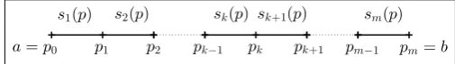
Problem formulation

Consider widely used and computationally simplest inter-polation spline of the third-degree. Also, we shall proceed from the assumption that knots of the splinepkare

a=p0, p1, p2, . . . , pm−1, pm=b, [a, b]∈R

such that

ξk =ξ(pk)∈C, k= 0,1, . . . , m

and besidesξ0=ξmis tangency condition (Figure 1).

Let us define a complex cubic spline as a piecewise-polynomial complex-valued function of a real variable:

S: [a, b]7→_C

The complex plane

ξ1 ξ3

ξk−1 ξk

ξk+1 ξ2

[image:2.595.301.537.90.151.2]

ξ0 ξm

Figure 1.The control pointsξk

on an interval [a, b] ⊂ _R composed of m subintervals [pk−1, pk]with

a=p0< p1< . . . < pm−1< pm=b

So, the complex cubic spline function is defined as

S(p)≡sk(p) =ak+bk(p−pk)+

+ck(p−pk)2+dk(p−pk)3,

(1) where

p∈[pk−1, pk]⊂R;

ak, bk, ck, dk∈C

k= 1,2, . . . , m,

obeying continuity conditions for the function itself and its first two derivatives:

I (interpolation conditions)

sk(pk) =ξk;

II (continuity conditions)

sk−1(pk−1) =sk(pk−1) s0_k−1(pk−1) =s

0

k(pk−1) s00_k−1(pk−1) =s

00

k(pk−1) 

  

  

k= 2,3, . . . , m

III (contact conditions in the pointξ0 = ξm) s1(p0) =sm(pm);

s0₁(p0) =s 0

m(pm);

s00₁(p0) =s 00

[image:2.595.300.516.408.593.2]

m(pm).

Figure 2 illustrates structure of the spline.

sk(p) sm(p)

pk−1 p2

p1 pk pk+1 pm−1 pm=b

a=p0

sk+1(p) s2(p)

s1(p)

Figure 2.Positioning of the knots and intervals.

Substituting functions

sk(p) =ak+bk(p−pk) +ck(p−pk)2+dk(p−pk)3

and their derivatives

s0k(p) =bk+ 2ck(p−pk) + 3dk(p−pk)2

[image:2.595.295.548.622.658.2]

into the continuity conditions and assuming for simplicity

hk=pk−pk−1, we obtain 

                   

                   

interpolation conditions I

ak=ξk, k= 1,2, . . . , m

continuity conditions II

ak−1=ak−bkhk+ckh2k−dkh3k bk−1=bk−2ckhk+ 3dkh2k ck−1=ck−3dkhk



 

 

k= 2,3, . . . m

contact conditions III

a1−b1h1+c1h21−d1h31=am

b1−2c1h1+ 3d1h21=−bm

c1−3d1h1=−cm

An obvious next step is to evaluate unknown coeffi-cientsak, bk, ck, dk from this system. We can eliminate the ak, bk, dkand reduce the problem in the unknownsck.

We write expression for finding the coefficients ck, but

reader is referred to the literature [20] for these more detailed formulations. Eliminatingak, bk, dkfrom this system gives

hk−1ck−2+2(hk−1+hk)ck−1+hkck=

= 3

_ξ

k−ξk−1 hk

−ξk−1−ξk−2

hk−1

,

k= 2,3, . . . , m.

(2)

A few general comments should be made about solving the system (2). Fork = 2coefficientc0 is involved in this

equation, which we put equal to zero (so-called, dummy co-efficient). In order to apply standard tridiagonal matrix al-gorithm, to solve this tridiagonal system of equations, coeffi-cientcmalso required is equal to zero. So, we first consider cm = 0, but, after the system (2) is solved, we expresscm

from the contact condition:cm= 3d1h1−c1. We do not take

into account the continuity condition for the1stderivative in the pointξ0=ξm:b1−2c1h1+3d1h216=−bm, (derivative at

point of contact (sharp edge) does not exist). This omission does not affect subsequent results. In this case, the complex cubic spline (1) just loses property to be a “natural”.

It must be noted, that |2hk−1 + 2hk| |hk−1| + |hk|, which means that there exist a single unique set of c1, c2, . . . , cm, satisfying (2).

2.2

Results of the approximation

Let us put thehk = 1for simplicity. In this case, system

(2) takes the form:

ck−2+ 4ck−1+ck= 3(ξk−2ξk−1+ξk−2), k= 2,3, . . . , m,

c0=cm= 0

(3)

Right sides of equations (3) are complex, while coefficient matrix is real. One may solve two systems for real and imag-inary parts of the right sides of equations separately (due to linearity) and combine these results to obtain solution for the

[image:3.595.66.290.121.276.2]

approximated airfoil control points

Figure 3.Approximated airfoil. Number of knots of the spline – 8. Number of points per interval – 30.

original system (3). Figure 3 demonstrates result of solving system (3).

Advantage of this method is possibility of varying the con-trol points to get a curve of arbitrary shape.

3

Vortex panel aerodynamic model

3.1

Mathematical formulation

This paper presents vibrations (flutter) of a particular seg-ment of an airfoil, and this requires a certain method of ap-proximation by the complex cubic spline. Airfoil contour is replaced by its approximated coordinates from the first chap-ter:

zk, k= 1,2, . . . , n+ 1, (z1=zn+1),

where

n=m×(number of points per interval)

and the vortex panel method was used to construct complex potential.

Introducing complex potential as superposition of uniform flow at an angle αand potential due to effects of vorticity field around the airfoil we obtain

w(z) =U∞e−iαz−

I

γ(s) ln(z−z(s))ds,

Un= 0,

(4)

where

w(z) — complex potential;

U∞ — free stream velocity;

γ(s) — vorticity field;

α — angle of attack;

Un= 0 — no penetration condition.

Here, i is imaginary unit and complex variable notation

z = x + iy is used. Unless otherwise stated, α = 0 andH. . . dsmeans integrating over the airfoil contour.

Complex conjugate velocityV is defined by

V = dw

dz =U∞− ∂ ∂z

I

γ(s) ln(z−z(s))ds (5) In order to prevent confusion, let us also define complex velocityU =V. So, we have

V =u−iv,

whereu, vare fluid velocity components.

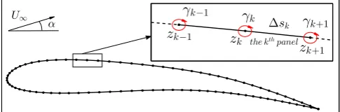
Replacement of continuous airfoil by its approximate co-ordinateszkfrom the first section gives polygon withnsides,

called “panels”. Let us number the panels clockwise with the 1st_{panel starting on lower side, at trailing edge and then}th

panel ending on trailing edge from upper side (Figure 4).

γk−1 _γ

k

zk+1

Δsk zk

γk+1 the kth_panel zk−1

[image:4.595.42.285.174.254.2]

U_∞ α

Figure 4.Arrangement of point vortices and control points for vortex panel aerodynamic model.

Assume that each panel represents a planar vortex sheet with linearly varying strength and such that end strength of each panel is the same as starting strength of the next panel:

γ(s) =γk+

(γk+1−γk)s

∆sk

;

z(s) =zk+

(zk+1−zk)s

∆sk

;

∆sk=|zk+1−zk|;

s∈[0,∆sk];

k= 1, . . . , n+ 1.

The only exception isγ16=γn+1.

Therefore, integral in right side of (5) may be computed analytically:

∂ ∂z

I

γ(s) ln(z−z(s))ds=

I _γ(s)

z−z(s)ds=

= 1 2πi

n

X

k=1 ∆sk Z

0

(γk+1−γk)s+γk∆sk

(z−zk)∆sk−(zk+1−zk)s ds

(6)

Evaluating integral (6) and substituting above expression into (5) gives

V =U∞−

1 2πi

n

X

k=1

∆sk zk+1−zk

γk+1−γk+

+

_(z−z

k)(γk+1−γk) zk+1−zk

+γk

lnz−zk+1

z−zk

(7)

The only unknowns of this problem are strengthsγk, k=

1, . . . , n+ 1. They can be found by solvingn+ 1equations consisting of

• n equations, expressing condition, that velocity at n

mid-points of the panels (called “collocation points”) is tangential to the panel;

• one equation

γ1+γn+1= 0

expressing the Kutta-Joukowski condition, which means, physically, that flow leaves sharp edge smoothly with no singularity. But, mathematically, it makes so-lution of Neumann boundary problem in outer region unique.

Collinearity condition of two complex numbersz1andz2

states

Re(iz1z2) = 0,

where Re(•)is real part.

Apply this condition at the n collocation points (mid-panels) (Figure 5)

zl0=

zl+1+zl

2 , l= 1, . . . n.

After various manipulations we obtain system of linear, al-gebraic equations

n

X

k=1

Re

∆sk

zl+1−zl zk+1−zk

γk+1−γk+

+

(z_l0−zk)(γk+1−γk) zk+1−zk

+γk

lnz

0 l −zk+1 z0

l −zk

=

=−Re(2πiU∞(zl+1−zl)),

(8)

wherel= 1, . . . , n.

Note, that fork=lin (8) we must take

k=l ⇒ lnz

0 l −zl+1 z0

l −zl

=πi.

It means that angle betweenz0

[image:4.595.64.281.607.665.2]

l −zl+1andz0l −zlequalsπ

(Figure 5).

airfoil midpoints z0

l+1

z0

l−1 z 0

l

zk+1

zk

zk−1 π

Figure 5.Collocation geometry of two-dimensional aerodynamic model.

To find solution of system (8) with satisfactory accuracy and adequate level of smoothness, we must take about one hundred points of approximation.

3.2

Nondimensionalization

Characteristic quantities to make equation (7) dimension-less are as follows:

c — airfoil chord;

U∞ — free stream velocity;

c U∞

— characteristic time;

ρ — air density;

1 2 0

[image:5.595.62.297.89.155.2]

c

U∞

Figure 6.Sketch of the problem.

3.3

Streamlines

Onceγ1, . . . , γn+1are known, we can find complex

veloc-ityU.

Let us consider an explicit Runge-Kutta method with second-order accuracy. Advancement from time instant t0

to the time instantt0+ ∆tin this method is made according

to the following expression:

zm+1=zm+

+∆t 2

U(zm) +U zm+ ∆t·U(zm)

, (9)

wherein as an initial condition one can take any pointz0

[image:5.595.77.551.364.443.2]

out-side airfoil contour, which streamline should be started with. Figure 7 demonstrates streamlines relative to airfoil.

Figure 7.Streamlines flow around airfoil.

4

Complex stream function

4.1

Complex potential

In previous chapter we obtained formula for complex con-jugate velocity (7). Let us integrate it with respect toz:

w(z) =

Z

V(z)dz=U∞z+

+ 1 2πi

n

X

k=1

∆sk

2Ak

Bk(zk+z)−CkAkln(z−zk+1)+

+(zk−z)(Ckzk−Bkz−2γkzk+1) ln

z−zk+1 z−zk

Ak

!

,

(10)

where

Ak =zk+1−zk;

Bk=γk+1−γk;

Ck=γk+1+γk.

For simplicity, in what follows, an integration constant in (10) will be omitted without essential loss of generality.

Principal difficulty of evaluatingw(z)by applying (10) is presence of logarithmic termln(z−zk+1).

4.2

Defining of single-valued branches

Complex logarithmic function is defined by

Ln(z) = ln|z|+iArg(z) = ln|z|+i(θ+ 2πk),

k∈Z.

Since infinitely different values ofArg(z)are obtained by successively encircling originz = 0, complex logarithmic function is infinitely multi-valued.

In any simply-connected domain there exist infinitely many single-valued branches of multi-valued complex log-arithm and its values ofArg(z)differ by integer multiples of 2π. And each such branch is a bijective function.

To keep the function single-valued, an artificial barrier that cannot be crossed must be introduced. This barrier is called branch cut, direction of which is arbitrary and largely a matter of convenience.

Let us divide entire flow domain, which is2 −connected, into two simply-connected domainsD+ andD−, boundary

of which consists of separatrix and the airfoil contour itself (Figure 8).

D

+

D

−

∂

Figure 8.Two simply-connected domains —D+andD−

Therefore, in each of these domains we can define single-valued branch ofLn(z−zk+1):

ln+(z−zk+1) = ln|z−zk+1|+iArg+(z−zk+1), z∈D+

ln−(z−zk+1) = ln|z−zk+1|+iArg−(z−zk+1), z∈D−

with following equality:

ln+(z−zk+1)−ln−(z−zk+1) =

=i(Arg+(z−zk+1)−Arg−(z−zk+1)) =−2πi

(11)

It was found, experimentally, that branch cuts ofln+ and

ln−are rays from origin to infinity at angles−π₂ and π₂,

re-spectively (Figure 9).

−π

2

π 2

A

Arg−

θ3=π+ tan−1y

x

θ2=π−tan−1y

x θ1= tan− 1y

x

θ4=−tan−1y

x θ4=−tan

−1y

x

θ1= tan−1yx

θ2=−π−tan−1yx

θ3=−π+ tan−1yx

Arg+

B

1 i

i

1

Figure 9. On calculation of principal values of the argumentsArg+ (A)

[image:5.595.59.287.571.729.2] [image:5.595.310.563.651.742.2]

So, among infinitely many branches of multi-valued func-tion (10) two single-valued branches were determined:

w+(z) =U∞z+

+ 1 2πi

n

X

k=1

∆sk

2Ak

Bk(zk+z)−CkAkln+(z−zk+1)+

+(zk−z)(Ckzk−Bkz−2γkzk+1) ln

z−zk+1 z−zk

Ak

!

,

z∈D+

(12)

and

w−(z) =U∞z+

+ 1 2πi

n

X

k=1

∆sk

2Ak

Bk(zk+z)−CkAkln−(z−zk+1)+

+(zk−z)(Ckzk−Bkz−2γkzk+1) ln

z−zk+1 z−zk

Ak

!

,

z∈D−.

(13)

4.3

Comparison of methods

Once complex velocityU is known, we can find scalar ve-locity potentialϕfrom condition, which states thatU =∇ϕ. Let us identify the velocity potentialϕas a function ofz(t) , wherez(t) = (x(t), y(t))is coordinates of fluid element along an arbitrary curve in whole flow domain at the time instantt.

Taking into account that ∂ϕ_∂t ≡0(steady flow), we obtain

ϕ(z(t+ ∆t))−ϕ(z(t))

∆t =

=dϕ

dt = ∂ϕ ∂x

dx dt +

∂ϕ ∂y

dy dt =U

2_,

(14)

Let us apply the same explicit Runge-Kutta scheme to in-tegrate the scalar velocity potential:

ϕm+1_−ϕm

∆t =

= 1 2

U2(zm) +U2(zm+ ∆tU(zm))

.

(15)

[image:6.595.299.547.88.266.2]

However, it should be noted that above formula can be used if only coordinates of the curve, along which the in-tegration is performed, are known a priori. Or, for example, these two recurrence relations (9) and (15) must be solved simultaneously forzm_andϕm_{with given∆t.}

Figure 10 demonstrates result of numerical integration scheme (15) with initial conditions ϕ0_± =Re[w±(s0±)],

(Fig. 10B), and two branches of scalar velocity potential, which were calculated by using (12) and (13), (Fig. 10C), along upper S+ and lower S− streamlines, respectively,

whereS±∈D±.

Agreement between these methods was found to be rea-sonably good. Difference between these two approaches is negligible and is of the order of1×10−7_.

ϕ−(z),z∈S−

ϕ+(z), z∈S+

D₋

D+

s0

+

s0

−

A

B

C

ϕ+(s0+)

ϕ−(s0

−)

S+∈D+

[image:6.595.42.282.112.347.2]

S−∈D−

Figure 10. Comparison of numerical Runge-Kutta scheme (B) with our analytical solutionϕ±(z) =Re[w±(z)](C).

4.4

Circulation

We know that circulationΓmay be calculated as Γ =ϕ+(zt.e.)−ϕ−(zt.e.),

wherezt.e.is trailing edge.

Consider the following expression Re[w+(zt.e.)−w−(zt.e.)]

or, given the fact thatw≡ϕ+iψ, whereϕ, ψ∈R,

it becomes

Re[w+(zt.e.)−w−(zt.e.)] =

=Re[ϕ+(zt.e.) +iψ+(zt.e.)−ϕ−(zt.e.)−iψ−(zt.e.)] =

=ϕ+(zt.e.)−ϕ−(zt.e.) = Γ,

in addition,ψ+(zt.e.)−ψ−(zt.e.)≡0, becausezt.e.is

coor-dinate of streamline (airfoil contour).

On the other hand, considering (12) and (13), we have

w+(zt.e.)−w−(zt.e.) =

=− 1

2πi n

X

k=1

∆sk

2 Ck(ln+(zt.e.−zk+1)−ln−(zt.e.−zk+1)) or, taking into account (11)

− 1

2πi n

X

k=1

∆sk

2 Ck(ln+(zt.e.−zk+1)−ln−(zt.e.−zk+1)) =

=− 1

2πi n

X

k=1

∆sk

2 Ck(−2πi) =

n

X

k=1

∆sk

2 Ck =

=

n

X

k=1

γk+γk+1

2 ∆sk,

where, obviously,Pn

k=1

γk+γk+1

2 ∆sk∈R.

Thus, we have obtained formula for the circulationΓ: Γ =

n

X

k=1

γk+γk+1

We may obtain absolutely the same result by integrating vorticity fieldγ(s)over the airfoil contour:

I

airfoil

γ(s)ds=

n

X

k=1 ∆sk Z

0

γk+

(γk+1−γk)s

∆sk

ds= = n X k=1

γks+

(γk+1−γk)s2

2∆sk

∆sk

0 = = n X k=1

γk+

γk+1−γk

2

∆sk = n

X

k=1

γk+γk+1

2 ∆sk.

Physical interpretation of (16): γk+γk+1

2 is average value

of complex velocity on thekthpanel.

5

Modelling of fluid-structure

interaction

5.1

2D aeroelastic design

For further description of airflow-structure interaction an idealized physical model of elastic airfoil design was devel-oped. Let us assume that all pointsz1, z2, . . . , zn+1 of the

airfoil are interconnected by elastic weightless rod to provide elastic deformation. The main purpose of this paper is nu-merical study of average lift force change caused by elastic vibrations of a segment of the airfoil (Figure 11).

[image:7.595.64.289.139.244.2]

To discuss these phenomena we must first develop dy-namic theoretical model.

Figure 11. Flutter geometry. Planar deformation of an elastic segment of airfoil.

Let us fix static (stationary) airfoil with its coordinates

z₁∗, z₂∗. . . z_n∗₊₁. In what follows, superscript ∗ is related to this stationary airfoil, which remains motionless in any time. Without loss of generality consider one of control points of the stationary airfoilξ_δ∗, by which airfoil contour was ap-proximated, and two adjacent pointsz∗_δ−iandz_δ∗_+i, which lie on both sides of theξ∗

δ (Figure 12).

f low _ξ∗

δ+ξδ

T2 Tres Fdyn l2 T1 n ξ∗ δ

z_δ−∗ _i z_δ∗_+i

l1

deformed elastic segment unstrained

[image:7.595.58.297.658.751.2]

elastic segment

Figure 12.Flow over a buckled elastic segment. Summation of forces acting on pointξ_δ∗+ ˆξδ.

Consider a small deviationξˆδof the pointξ∗δfrom its initial

position, after which the point moves toξ∗_δ+ ˆξδ. At the same

time we believe, that pointsz∗

δ−iandzδ∗+istay in their same

locations. Describe motion of the disturbed pointξδ by the

following equations:

ξδ(t+ ∆t) =ξδ(t) + ∆tvδ

t+∆t 2

, (17)

vδ

t+∆t 2

=vδ

t−∆t

2

+ ∆taδ(t), (18)

with initial conditions which are natural from viewpoint of the experiment:

ξδ(0) =ξδ∗+ ˆξδ; (19)

vδ(0) = 0; (20)

aδ(0) =

1

mFδ(0); (21)

vδ(∆t/2) =vδ(0) + (∆t/2)aδ(0), (22)

whereFδ is resultant force acting on theξδ; coefficient m

represents measure of inertia of an oscillating segment. It should be noted that this deviationξˆδ must be the same

order as the arc length of airfoil:

|ξˆδ| ∼=|zδ∗+i−ξδ∗| ∼=|ξδ∗−z∗δ−i|.

Next step is to find all external applied forces and internal elastic forces acting on the pointξδ. Neglecting gravity, it

is clear that major contribution to the total motion is made by aerodynamic pressureFdyn(force per unit arc length) and

tension forceTres(Figure 12).

5.2

Resultant vector Tres

We put parameteri= 1. Now we must express the resul-tant forceTresin terms of thezδ∗−1, ξ

∗

δ, z

∗

δ+1andξ

∗

δ+ ˆξδ. All

explanations will be carried out for T1 (Figure 12), forT2

analogous reasoning leads to similar result. Hooke’ s Law reads

|T1| ∼

z_δ∗₊₁−(ξ_δ∗+ ˆξδ)

−

z_δ∗₊₁−ξ∗_δ

z_δ∗₊₁−ξ∗_δ

,

or

|T1|=E   z ∗

δ+1−(ξδ∗+ ˆξδ)

z_δ∗₊₁−ξ∗_δ −1  , where

|z∗_δ+1−(ξ∗_δ+ ˆξδ)| |z∗

δ+1−ξ

∗ δ|

−1

is relative elongation (deforma-tion) of the arc length betweenξ∗_δ andz_δ∗₊₁,Eis modulus of elasticity.

We obtain

T1=|T1|l1,

wherel1= z∗

δ+1−(ξ

∗ δ+ ˆξδ) |z∗

δ+1−(ξδ∗+ ˆξδ)|

is unit vector. Therefore

1 1.169 2

−0.089 ξ

[image:8.595.78.502.87.450.2]

∗ δ

Figure 13.Oscillating control pointξ∗ δ.

1.16924 1.1693 1.16934 1.16938

−0.09 −0.088 −0.086 −0.084 −0.082 −0.08 −0.078

x

y

ξ∗ δ

ξ∗ δ+ξδ

A

1.16926 1.16932 1.16936

−0.0834 −0.0834 −0.0834 −0.0834 −0.0834

x

y

B

20 30 40 50 60 70 80 90 100

0.7307 0.7308 0.7309 0.731

t

ϕ

(

ξ

∗,tδ

)

100 101 102 103 104 105

0.7308 0.7309

t

ϕ

(

ξ

∗,tδ

)

C

Figure 14. Time evolution of control pointξδfrom time instantt= 0(A) and from some later time (B). Damped oscillations of nondimensional scalar velocity potentialϕat the vibrating pointξδ(C).U∞= 1,E= 1. Inset shows that solution of stability problem (17)-(22) has adequate level of smoothness.

5.3

Dynamic pressure. The Cauchy-Lagrange integral

This perturbationξˆδ triggers an aerodynamic flow so that

now we have to take into account unsteady motion near the oscillating segment.

Cauchy-Lagrange integral may serve for the same purpose as Bernoulli’s equation. If potential of velocityϕis known then pressure may be found with the aids of this integral. The practical value of Cauchy-Lagrange integral is that it allows one to relateptoϕ. Using it we obtain

∂ϕ ∂t +

U2

2 +

p

ρ=f(t).

We may evaluatef(t)by examining fluid at some point where we know its state. For example, far away from body. Thenf(t)becomes U∞2

2 +

p∞

ρ ≡f∞and we find thatf∞is

a constant independent of space and time. Hence finally

∂ϕ ∂t +

U2

2 +

p ρ=f∞.

Let us express pressurep:

p=−ρ

_∂ϕ

∂t + U2

2 −f∞

. (23)

However, to describe motion of theξδwe need total

deriva-tive ofϕwith respect tot:

dϕ dt =

∂ϕ ∂t +

∂ϕ ∂x

dx dt +

∂ϕ ∂y

dy

dt (24)

Expressing from (24) partial derivative:

∂ϕ ∂t =

dϕ dt −

_∂ϕ

∂x dx

dt + ∂ϕ ∂y

dy dt

= dϕ

dt −U 2

and substituting it into (23) gives

p=ρ

_U2

2 −

dϕ dt +f∞

Thus

Fdyn=ρ _U2

2 −

dϕ dt +f∞

n

_ξ∗

δ+ ˆξδ ·c

3,

[image:8.595.296.532.527.727.2]

50 100 150 200 250 300 0.734

0.7341

t

ϕ

(

ξδ

,t

)

1.1693 1.1694 −0.082

−0.081

x

y

U∞= 3

A

140 160 180 200 220 240 260 280 300 320 0.7366

0.7367

t

ϕ

(

ξδ

,t

)

304 306 308 310 312 314 0.736611

0.736612

t

ϕ

(

ξδ

,t

)

1.1691 1.1693 1.1695 −0.081

−0.08

x

y

U_∞∗ = 3.558

B

100 150 200 250 300 0.738

0.739

t

ϕ

(

ξδ

,t

)

1.1685 1.17

−0.08 −0.079

x

y

U∞= 4

[image:9.595.142.468.83.390.2]

C

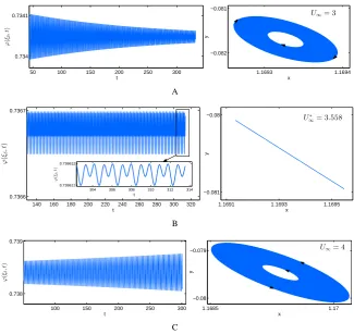
Figure 15.Transient response leading to a limit cycle oscillation. Nondimensional scalar potentialϕ(ξδ, t)vs nondimensional time,t, for different values ofU∞together with motion path of the perturbed point. (A) Decaying amplitude of potential forU∞= 3, (C) growing amplitude forU∞= 4and (B) limit cycle oscillation forU∗

∞≈3.558. Inset illustrates typical period doubling bifurcation. For all calculations,E= 1.

6

Simulation Results

In this section, results of simulation will be analysed us-ing theory of aerodynamic stability and nonlinear dynamical systems. Unless otherwise stated,m = 1, ρ = 1and as in-vestigated control pointξ_δ∗ we take one of control points of lower surface of airfoil (Figure 13).

6.1

2D solution and its stability

Simulations showed (Figure 14) that for relatively small values of free stream velocityU∞stable solutions of the

sys-tem (17)-(22) are realized.

For the control parameterU∞=U∞∗ and fixedE, solution

of (17)-(22) suffers a bifurcation (Fig. 15B). This system has a phase space, and it was crucial for its understanding to choose proper projection of this space. So, in order to clarify the behaviour of the system, it was instructive to consider trajectories of perturbed pointξδ.

In stable case,U∞ < U∞∗, phase trajectory att → ∞is

attracted to some fixed point, stable focus (Fig. 15A, right), and with increasingU∞,U∞ > U∞∗, solution becomes

un-stable, unstable focus (Fig. 15C, right).

Numerical simulations of (17)-(18) with initial conditions (19)-(22) confirmed birth of a stable cycle. This is illustrated in Fig. 15B (left), where it is shown that the solution acquired periodic oscillations in time. It is interesting to note, that trajectory of perturbed point, in this case, takes form of a straight segment (Fig. 15B, right).

This attracting-repelling scenario ran over many times. However, it is not our purpose to probe deeply into this prob-lem here; for a thorough treatment reader is referred to Dow-ell [11] and Bolotin [21]. The reader may wish to consider another specific issues of the theory of aeroelastic instability (see, for example, Vedeneev, Shishaevaet al.[22–31])

Fig. 16A demonstrates a family of plots for various values

E where oscillations of scalar potential are presented. One can see that mean values of oscillations, as modulus of elas-ticity increases, tend to their limiting value of potential of steady-state airfoil in pointξ_δ∗(Fig. 16B).

6.2

Lift

It is interesting to examine total force (lift)Lon this aeroe-lastic effect. Pressure distribution (23) may be integrated along airfoil contour to obtain the total force (lift) on a wing:

L(t)≡ I

airfoil

pnds=ρ

I

airfoil

_U2

2 −

dϕ dt

n·ejds, (25)

wherenis normal unit vector pointing into the wing and

ejis vertical unit vector, normal to freestream direction.

In our case (α= 0), we haveej ≡iand (25) becomes L(t) =−ρ

I

airfoil

U2

2 −

dϕ dt

nyds, (26)

so that nownyisy-component of outward-pointing unit

86 88 90 92 94 96 98 100 102 104 0.722

0.723 0.725 0.728 0.731 0.735 0.745

t

ϕ

(

ξδ

,t

)

0 1.16925 3

−1 0.718 2 3

s ϕ±

(

s

)

E= 0.5

E= 1

E= 2

E= 0.2

A B

E= 10

E= 20

[image:10.595.109.477.86.253.2]

E= 5

Figure 16.(A) Oscillations of potentialϕ(ξδ, t)for differentE. (B) Value of scalar potential of steady-state airfoil in the pointξδ∗.U∞= 1.

t

0 20 40 60 80 100

|

L

(

t

)

|

[image:10.595.154.430.283.368.2]

1.403 1.443

Figure 17.Effect of vibration on lift amplitude. Red line is lift of steady-state airfoil. Blue graph shows oscillations of the total lift (26).U∞= 1,E= 1.

Figure 17 shows that change of the total lift force is about 3% of lift force of steady-state airfoil.

7

Conclusions

Results of numerical simulation of aerodynamic instabil-ity, within context of airflow-structure interaction, were pre-sented and understood from viewpoint of bifurcation and sta-bility theory. In context of nonlinear system theory, a limit cycle oscillation LCO is one of the simplest dynamic bifur-cations, “a first stop on the road to chaos”, so to speak.

Despite the fact that we considered a highly simplified model (somewhat analogous to elastic design of an airfoil), it was possible to bring out some of essential features of this type of problem, thus the model serves a useful purpose in introducing this type of flutter.

In this paper, oscillations of airfoil segment have a natural (uncontrolled) character, so that they provides an insignifi-cant augmentation of lift force. Up to a certain magnitude of deviation of the perturbed point oscillations result in a trans-fer of energy from flow to body. This transtrans-fer may be viewed as equivalent to a flow-induced negative aerodynamic damp-ing. For larger deviations, however, there occurs a transfer of energy from the body to the airstream. Control of this process with the aim of more effective increasing of total lift force is the main purpose of next studies.

Optimal mechanism of the interaction for energy transfer from airstream to oscillating airfoil should include at least two oscillating segments on lower and upper surfaces of a wing. This mechanism should be able to control both

dissi-pation and forced oscillations of segments themselves. This control implies a specific connection between the fric-tion forces and flow-induced forces, acting on oscillating sec-tions of airfoil, to pump energy from airstream into vibration and thus sustain the presumed motion.

REFERENCES

[1] T.K. Lifanov, T.E. Polanski. Proof of the numerical method of Discrete Vortices for solving singular integral equations. PMM, pp. 742-746, 1975.

[2] E. Albano, W.P. Rodden. A doublet-lattice method for cal-culating lift distributions on oscillating surfaces in subsonic flows. AIAA J 7(2), pp. 279-285, 1969.

[3] W.P. Rodden, J.P. Giesing, T.P. Kalman. New developments and applications of the subsonic doublet-lattice method for non-planar configurations. AGARD symposium on unsteady aerodynamics for aeroelastic analyses of interfering surfaces, Tonsberg, Oslofjorden, Norway, 34, Nov 1970.

[4] K.M. Roughen, M.L. Baker, T. Fogarty. Computational fluid dynamics and doublet-lattice calculation of unsteady control surface aerodynamics. J. Aircr 24(1), pp. 160-166, 2001.

[5] W.P. Rodden. A comparison of methods used in interfering lifting surface theory. AGARD Report R-643, March 1976.

[7] S.S. Davis, G.N. Malcolm. Transonic shock-wave/boundary layer interactions on an oscillating airfoil. AIAA J 18(11), pp. 1306-1312, 1980.

[8] E.H. Dowell. A modern course in aeroelasticity, Solid me-chanics and its applications. Springer International Publish-ing, Switzerland, pp. 495-504, 2015.

[9] Y.C. Fung. On two-dimensional panel flutter. J. Aero/Space Sci. 25(3), pp. 145-159, 1958.

[10] S. Kobayashi. Two-dimensional panel flutter 1. Simply sup-ported panel. Trans. Japan Society Aeronautical Space Sci-ences 5(8), pp. 90-102, 1962.

[11] E.H. Dowell. Aeroelasticity of plates and shells. Noordhoff International Publishing, Groningen, 1975.

[12] E.H. Dowell. Flutter of a buckled plate as an example of chaotic motion of a deterministic autonomous system. J. Sound Vib. 85(3), pp. 333-344, 1982.

[13] A. Kornecki. Static and dynamic instability of panels and cylindrical shells in subsonic potential flow. J. Sound Vib. 32, pp. 251-263, 1974.

[14] A. Kornecki, E.H. Dowell, J. O’Brien. On the aeroelastic in-stability of two-dimensional panels in uniform incompressible flow. J. Sound Vib. 47, pp. 163-178, 1976.

[15] V.V. Vedeneev. Panel flutter at low supersonic speeds. Journal of Fluids and Structures, Vol. 29, pp. 79-96, 2012.

[16] V.V. Vedeneev, S.V. Guvernyuk, A.F. Zubkov, M.E. Kolot-nikov. Experimental observation of single mode panel flutter in supersonic gas flows. Journal of Fluids and Structures, Vol. 26, pp. 764-779, 2010.

[17] V.V. Vedeneev. Nonlinear high-frequency flutter of a plate. Fluid Dynamics, No.5, pp. 858-868, 2007.

[18] V.V. Vedeneev. High-frequency flutter of a rectangular plate. Fluid Dynamics, No.4, pp. 641-648, 2006.

[19] V.V. Vedeneev. High-frequency plate flutter. Fluid Dynamics, No.2, pp. 313-321, 2006.

[20] V.M. Vierzhbitsky. Basics of numerical methods. Vysshaya shkola, pp. 441-442, 2002. (in Russian)

[21] V.V. Bolotin. Non-conservative problems of the elastic theory of stability. Pergamon Press, Oxford, 1963.

[22] V.V. Vedeneev. On the application of the asymptotic method of global instability in aeroelasticity problems. Proceedings of the Steklov Institute of Mathematics, Vol. 295, pp. 274-301, 2016.

[23] V. Bondarev, V. Vedeneev. Short-wave instability of an elastic plate in supersonic flow in the presence of the boundary layer. Journal of Fluid Mechanics, Vol. 802, pp. 528-552, 2016.

[24] V.V. Vedeneev. Propagation of waves in a layer of a viscoelas-tic material underlying a layer of a moving fluid. Journal of Applied Mathematics and Mechanics, Vol. 80, Issue 3, pp. 225-243, 2016.

[25] A. Shishaeva, V. Vedeneev, A. Aksenov. Nonlinear single-mode and multi-single-mode panel flutter oscillations at low super-sonic speeds. Journal of Fluids and Structures, Vol. 56, pp. 205-223, 2015.

[26] A. Shishaeva, V. Vedeneev. Evolution of nonlinear panel flut-ter oscillations. Visualization of mechanical processes. An In-ternational Online Journal, Vol. 3, Issue 1, pp. 205-223, 2013.

[27] V. Vedeneev. Interaction of panel flutter with inviscid bound-ary layer instability in supersonic flow. Journal of Fluid Me-chanics, Vol. 736, pp. 216-249, 2013.

[28] V.V. Vedeneev. Effect of damping on flutter of simply sup-ported and clamped panels at low supersonic speeds. Journal of Fluids and Structures, Vol. 40, pp. 366-372, 2013.

[29] V.V. Vedeneev. Limit oscillatory cycles in the single mode flutter of a plate. Journal of Applied Mathematics and Me-chanics, Vol. 77, Issue 3, pp. 257-267, 2013.

[30] V.V. Vedeneev. Coupled-mode flutter of an elastic plate in a gas flow with a boundary layer. Proceedings of the Steklov Institute of Mathematics, Vol. 281, pp. 140-152, 2013.