arXiv:hep-th/0307191v3 24 Aug 2003
AEI-2003-059 Imperial/TP/2-03/28
hep-th/0307191
Spinning strings in
AdS
5×
S
5and integrable systems
G. Arutyunov1,⋆,∗, S. Frolov2,⋆, J. Russo3,4 and A.A. Tseytlin2,3,†
1 Max-Planck-Institut f¨ur Gravitationsphysik, Albert-Einstein-Institut,
Am M¨uhlenberg 1, D-14476 Golm, Germany
2 Department of Physics, The Ohio State University,
Columbus, OH 43210-1106, USA
3 Blackett Laboratory, Imperial College, London, SW7 2BZ, U.K.
4 Departament ECM, Facultat de F´ısica, Universitat de Barcelona
Instituci´o Catalana de Recerca i Estudis Avan¸cats (ICREA), Spain
Abstract
We show that solitonic solutions of the classical string action on the AdS5×S5
background that carry charges (spins) of the Cartan subalgebra of the global symme-try group can be classified in terms of periodic solutions of the Neumann integrable system. We derive equations which determine the energy of these solitons as a func-tion of spins. In the limit of large spins J, the first subleading 1/J coefficient in the expansion of the string energy is expected to be non-renormalised to all orders in the inverse string tension expansion and thus can be directly compared to the 1-loop anomalous dimensions of the corresponding composite operators inN = 4 super YM theory. We obtain a closed system of equations that determines this subleading coef-ficient and, therefore, the 1-loop anomalous dimensions of the dual SYM operators. We expect that an equivalent system of equations should follow from the thermody-namic limit of the algebraic Bethe ansatz for the SO(6) spin chain derived from SYM theory. We also identify a particular string solution whose classical energy exactly reproduces the one-loop anomalous dimension of a certain set of SYM operators with two independent R charges J1, J2.
∗emails: [email protected]; [email protected]; frolov, tseytlin @mps.ohio-state.edu
⋆
On leave of absence from Steklov Mathematical Institute, Gubkin str.8, 117966, Moscow, Russia
1
Introduction and summary
Recently, there was a remarkable progress towards understanding AdS/CFT duality in non-supersymmetric sector of states of string theory on AdS5 × S5 [1, 2, 3, 4],
generalizing earlier work of [5, 6, 7]. On the string side, one identifies semiclassical states described by solitonic closed-string solutions on a 2-cylinder. They have finite energy and carry SO(6) (and, in general, SO(2,4)) angular momentum componentsJi. In the limit of large angular momenta the first subleading term in the expansion of the classical string energies happens to be protected (i.e. is not renormalised by stringα′
corrections) and thus can be matched onto the dimensions of the corresponding gauge-theory (N = 4 SYM) operators [3]. We refer to [4] for a more detailed discussion.
In general, according to the AdS/CFT duality the AdS5×S5 string sigma model
should be equivalent to theN = 4 supersymmetric SU(N) YM theory withN → ∞. The composite primary operators in this theory are classified in terms of UIR’s of the superconformal group PSU(2,2,|4), i.e. by the conformal dimension ∆, two spins
S1, S2 and by the Young tableaux (or, equivalently, by the Dynkin labels) of the
R-symmetry group SU(4). At N = ∞ only single-trace operators matter. Thus one should expect that the energy of the string solutions considered as the function of the angular momenta Ji should match with the dimensions of the corresponding primary single-trace operators in the SYM theory.
The bosonic part of the classical string action is a combination of SO(2,4) and SO(6) sigma models. The O(n) (or O(p,q)) sigma models are known to be classically integrable [8], and the same should obviously be true also upon imposition of the conformal gauge constraints, i.e. for the corresponding classical string theories (for some related work see [9, 10, 11]). One expects, therefore, a close connection between special classes of string solutions representing particular semiclassical string states and certain integrable models. As was already observed earlier, the folded rotating string solutions with one [12, 6] or two [7, 4] non-vanishing angular momenta are related to the 1-d sine-Gordon model.
Here we will consider a generalization to the case when all the three “Cartan” components of the SO(6) angular momentum are non-zero and will find that in this case the SO(6) sigma model effectively reduces to a special integrable 1-d model –
theNeumann model[13]. The latter describes a three-dimensional harmonic oscillator
with three different frequencies constrained to move on a two- sphere (see, e.g., [14, 15, 16]).
The class of S5 rotating string solutions we will be discussing is parametrized by
the angular momenta Ji = (J1, J2, J3) with the energy being E = E(J1, J2, J3). To
be able to compare to perturbative conformal dimensions on the SYM side one needs to assume that
λ J2
i
≪1 , 1
Ji ≪
1, (1.1)
suppressed by extra powers of 1
Ji. This happens [2] despite the non-BPS nature of the extended rotating string states (the only BPS state is a point-like string having only one non-zero component of Ji [5]) and is due to the fact that the underlying superstring theory has (i) global supersymmetry and (ii) is effectively massive in this case (with 2-d masses ∼ 1
Ji)
1.
Assuming (1.1), the classical energy can be expanded as2
E =Jtot+
λ Jtot
f1(
Ji
Jtot
) + λ
2
J3 tot
f2(
Ji
Jtot
) +... , (1.2)
Jtot ≡J1+J2+J3 . (1.3)
One immediate aim is then to determine the coefficient function f1(JJtot2 ,
J3
Jtot). Given
the analytic dependence of the subleading term in E on λ and its expected “non-renormalizability” on the string side, one may be able, as explained in [2, 4], to compare it directly to the one-loop anomalous dimensions of gauge-theory operators of the type tr[(Φ1 +iΦ2)J1(Φ3 + iΦ4)J2(Φ5 + iΦ6)J3]+... belonging to irreducible
representation of SU(4) with Dynkin labels [J2−J3, J1−J2, J2+J3] (we assume for
definiteness thatJ3 ≤J2 ≤J1).3 Note also that the expected non-renormalisation of
the 1/Jtot term to all orders in the inverse string tension predicts (through AdS/CFT
duality) that the corresponding term in N = 4 SYM should be one loop exact. Finding the spectrum of one-loop anomalous dimensions of such scalar operators with all three Ji being non-zero should be possible, as in the two-spin case (J3 = 0)
in [3], using the techniques (dilatation operator related to integrable spin chains and Bethe ansatz) developed in a recent remarkable series of papers [19, 20, 3, 21]. Here we will determine f1 in several special cases with Ji 6= 0, thus making string-theory predictions for the corresponding eigenvalues of the anomalous dimension matrix.
One special three-spin solution was found already in [1, 2]: this is a circular string with J1 = J2 and arbitrary J3 (the stability condition implies J1 +J2 ≤ (24nn−−1)12J3
where n is the winding number; in what follows we set n = 1)
E =J1+J2+J3+
λ(J1 +J2)
2(J1+J2+J3)2
+...
1A similar argument explains [7, 17] why 2- and higher loop corrections to the energy of string
states in the BMN [5] sector are suppressed by powers of 1/J.
2In the cases when there is just one non-vanishing component of the spin as in [6] or the conditions
(1.1) are not satisfied for at least one of the spins [7, 18], the energy may contain also a constant subleading termO(√λ). Under the condition√λ
J ≪1 such term (which will not be protected against
stringα′ ∼ √1
λ-corrections and thus cannot be easily compared to SYM theory) is much larger that
the subleading term in the equation below, and thus the corresponding SYM operators should have larger anomalous dimensions.
3The primary operators obtained after diagonalizing the dilatation matrix for the gauge-invariant
operators mentioned above are not superconformal primaries lying on the unitary bound of the
= Jtot+
λ
2Jtot
(1− J3
Jtot
) +... , (1.4)
where dots stand forλ2 and other subleading terms. The special case of J
3 = 0, i.e.
E =J1+J2+f1
λ J1+J2
+... , f1 =
1
2 (1.5)
corresponds to the simplest two-spin circular string solution [1]. In spite of being unstable, this solution has its “counterpart” on the SYM side [3]. Another string state with the same quantum numbers J1 =J2, J3 = 0 but lower energy is represented by
the stable folded string solution [4] (which generalizes the single-spin solution of [6] to the two-spin case). In this case the energy is given by (1.5) with4
f1 = 0.356... ,
and, remarkably, can be matched exactly with the corresponding lowest anomalous dimension eigenvalue on the SYM side [3].
As in the two-spin case, in general, there will be several three-spin string solutions for given values of J1, J2, J3 having different values of E. The first subleading term
in E will then be expected to correspond to the band of one-loop dimensions of the SYM eigen-operators in the [J2−J3, J1−J2, J2+J3] irrep. In particular, there may
be several string solutions with J1 = J2 and small J3 generalizing the circular [1, 2]
and folded [4] two-spin solutions, and different from the circular string solution of [2] with E given in (1.4).
We shall see that in spite of the formal integrability of the Neumann model, finding the explicit form of the three-spin solutions and, in particular, their energies, turns out to be complicated. Below we shall concentrate on several special cases. In particular, there are two obvious cases generalizing the two-spin solutions mentioned above: (i) generalization of the folded two-spin solution to the case of non-zeroJ3 < J1 =J2; (ii)
generalization of the circular two-spin solution to the case of non-zero J3 < J1 =J2
which has less energy than the circular three-spin solution of [2] (the latter is unstable for small J3). In these and similar cases with J1, J2 ≫ J3 we find the following
expression for the energy (to the leading order in J3
Jtot)
E =Jtot+
λ Jtot
(f1(0)+f (1) 1
J3
Jtot
+...) +... . (1.6)
Note that the expression (1.4) for the circular three-spin solution of [2] is thus a special case of (1.6).5 One of our aims will be to compute the value of the coefficient f(1)
1 for
4This number has a simple origin in terms of values of elliptic functions as mentioned at the end
of Section 3.3.
5Let us mention that a reason for considering linear inJ
3terms in E (i.e. leading deformations
various three-spin solutions. In particular, we will find in Section 3 that the folded string solution that generalizes theJ1 =J2, J3 = 0 solution of [4] hasf1(1) = 4.79....
One may try to find also folded string solutions with J1 =J2 =J3, which should
have less energy than the circular solution of [2]. Though the latter is stable for
J1 =J2 =J3, it is likely to be only a local minimum of the energy, i.e. there may be
anotherJ1 =J2 =J3 solution with less energy.6
The rest of the paper is organized as follows. In Section 2 we shall present the ansatz for the general three-spin S5 rotating string solution and explain its relation
to the Neumann integrable system. This will allow us to reduce the problem to a pair of first-order differential equations for the two coordinates ofS2 related to 5-th order
polynomial defining a hyperelliptic curve of genus 2.
In Section 3.1 we shall argue that to obtain a non-trivial folded string solution with the three non-zero spins the string must be “bent” (i.e. two coordinates of S2
should have a different number of folding points). In Section 3.2 we shall derive the general system of equations that governs the form of the subleading (or “one-loop”) termf1 in the expression (1.2) for the energy of the bent string. An equivalent system
is expected to follow from the thermodynamic limit of the algebraic Bethe ansatz for the SO(6) spin chain determining the one-loop anomalous dimensions on the SYM side [19, 21]. In Section 3.3 we shall study this system in expansion in small J3 and
determine the coefficientf1(1) in (1.6) in the special case of perturbation near two-spin folded string solution of [4] with J1 =J2.
Section 4 will be devoted to a different class of three-spin solutions which will have higher energy than folded bent strings for the same values ofJi. Using a combination of analytic and numerical methods we shall again determine the form of the leading correction f1 in (1.2) in this case.
In Section 5 we shall consider a two-spin solution of a circular type that generalizes the circular solution of [1] to the case of unequalS5 spins (J
1, J2). We shall show that,
just in the case of the two-spin folded string in [4], the first subleading term in the corresponding expression for the energy matches precisely the one-loop anomalous dimensions of a set of SYM operators with SU(4) Dynkin labels [J2, J1−J2, J2] which
correspond to solutions of the Bethe ansatz equations in [3] with all Bethe roots lying on the imaginary axis. This complements the results in [3, 4], providing another remarkable test of the AdS/CFT correspondence.
Similar solutions describing string spinning in AdS5 directions can be analysed
in much the same way as described in Section 6. In fact, most of the SO(6) case equations have a direct analog in the SO(2,4) case or are related by an analytic continuation.
In Appendix A we shall explain how the general solution of the Neumann model can be written in terms ofθ-functions defined on the Jacobian of a hyperelliptic genus 2 Riemann surface [16]. Appendix B will contain a list of integrals used in Section 3. In 6In general, there may be several local minima, i.e. stable solutions with the same quantum
Appendix C we shall study the vanishing of other (“non-Cartan”) components of the SO(6) angular momentum tensor for different three-spin solutions which is crucial [1] for their consistent semiclassical quantum state interpretation (and thus a possibility to establish a correspondence with particular SYM operators with the same quantum numbers). In Appendix D we shall describe the two-spin solution corresponding to the straight folded string without bend points. We will show that such string solution does not allow a deformation towards a non-zero third spin component.
2
Reduction of O(6) sigma-model to the
Neumann system
2.1
Rotating string ansatz and integrals of motion
Let us consider the bosonic part of the classical closed string propagating in the
AdS5×S5 space-time. The world-sheet action in the conformal gauge is
I =−
√
λ
4π Z
dτ dσ [G(AdS5)
mn (x)∂axm∂axn + G(S
5
)
pq (y)∂ayp∂ayq],
√
λ≡ R
2
α′ . (2.1)
The two metrics have the standard form in terms of the 5+5 “angular” coordinates: (ds2)
AdS5 =−cosh
2ρ dt2+dρ2+ sinh2ρ (dθ2 + sin2θ dφ2+ cos2θ dϕ2) , (2.2)
(ds2)S5 =dγ2+ cos2γ dϕ2
3+ sin2γ (dψ2+ cos2ψ dϕ21+ sin2ψ dϕ22) . (2.3)
It is convenient to represent (2.1) as an action for the O(6)×SO(4,2) sigma-model (we follow the notation of [1])
I =
√
λ
2π Z
dτ dσ(LS+LAdS), (2.4)
where
LS = −
1
2∂aXM∂ aX
M + 1
2Λ(XMXM −1), (2.5)
LAdS = −
1
2ηM N∂aYM∂ aY
N + 1
2Λ(˜ ηM NYMYN + 1). (2.6) Here XM, M = 1, . . . ,6 and YM, M = 0, . . . ,5 are the the embedding coordinates of R6 with the Euclidean metric in L
S and with ηM N = (−1,+1,+1,+1,+1,−1) in
LAdS respectively. Λ and ˜Λ are the Lagrange multipliers. The action (2.4) is to be supplemented with the usual conformal gauge constraints.
The embedding coordinates are related to the “angular” ones in (2.2),(2.3) as follows:
X1+iX2 = sinγ cosψ eiϕ1 , X3+iX4 = sinγ sinψ eiϕ2 , X5+iX6 = cosγ eiϕ3 ,
Y1+iY2 = sinhρ sinθ eiφ, Y3+iY4 = sinhρ cosθ eiϕ, Y5+iY0 = coshρ eit. (2.8)
In the next few sections we will be discussing the case when the string is located at the center ofAdS5and rotating inS5, i.e. is trivially embedded inAdS5 asY5+iY0 =eiκτ
with Y1, ..., Y4 = 0.
The S5 metric has three commuting translational isometries inϕ
i which give rise to three global commuting integrals of motion (spins) Ji. Since we are interested in the periodic motion with threeJi non-zero it is natural to choose the following ansatz for XM:
X1+iX2 =x1(σ) eiw1τ, X3+iX4 =x2(σ) eiw2τ, X5+iX6 =x3(σ)eiw3τ, (2.9)
where the real radial functionsxiare independent of time and should, as a consequence of X2
M = 1, lie on a two-sphere S2:
3
X
i=1
x2i = 1 , i= 1,2,3.
Then the spins J1 = J12, J2 =J34, J3 = J56 forming a Cartan subalgebra of SO(6)
are
Ji = √
λ wi
Z 2π
0
dσ
2π x
2
i(σ)≡ √
λ Ji. (2.10)
As discussed in [1], to have a consistent semiclassical string state interpretation of these configurations one should look for solutions for which all other components of the SO(6) angular momentum tensor JM N vanish.
The space-time energy E of the string (related to a generator of the compact SO(2) subgroup of SO(4,2)) is simply
E =√λ κ≡√λ E. (2.11)
The only non-trivial Virasoro constraint is then (dot and prime are derivatives over
τ and σ)
κ2 = ˙XMX˙M +XM′ XM′ . (2.12) As a consequence of this relation the energy becomes a function of the SO(6) spins:
E =E(J1, J2, J3). (2.13)
Substituting the ansatz (2.9) into the SO(6) Lagrangian (2.5) we get the following 1-d (“mechanical”) system
L= 1
2
3
X
i=1
(x′2
i −wi2x2i) + 1 2Λ(
3
X
i=1
x2i −1). (2.14)
It describes ann= 3 dimensional harmonic oscillator constrained to remain on a unit
n−1 = 2 sphere. This is the special case of the n-dimensional Neumanndynamical system [13] which is known to be integrable [14].
The Virasoro constraint implies that the energyHof the Neumann system is given by
H = 1
2
3
X
i=1
(x′i2+w2ix2i) = 1 2κ
2. (2.15)
Solving the equation of motion for the Lagrange multiplier Λ we obtain the following non-linear equations forxi:
x′′
i =−wi2xi−xi
3
X
j=1
x′2
j −w2jx2j
. (2.16)
The canonical momenta conjugate toxi are
πi =x′i ,
3
X
i=1
πixi = 0.
One can think about this dynamical system as being originally defined on the cotan-gent bundle T∗R3 . Imposing the constraints reduces the phase space to T∗S2. The
Dirac bracket obtained from the canonical structure {πi, xj}=δij is
{πi, πj}D =xiπj −xjπi, {πi, xj}D =δij −xixj, {xi, xj}D = 0. (2.17) One can check that (2.16) follows from the Poisson structure (2.17) and the Hamil-tonian
H= 1
2
3
X
i=1
(π2i +w2ix2i) (2.18)
supplemented with the two constraintsP3
i=1x2i = 1,
P3
i=1πixi = 0.
The crucial point allowing to solve this model is that then-dimensional (n= 3 in the present case) Neumann system has the following n integrals of motion [22]:
Fi =x2i +
X
j6=i
(xiπj−xjπi)2
w2
i −wj2
,
n
X
i=1
In the present case n = 3 and thus only two of the three integrals of motion are independent. Moreover, these integrals are in involution with respect to the Poisson bracket (2.17) and the Hamiltonian is
H = 1
2
3
X
i=1
w2
iFi . (2.20)
Thus, any two of these three integrals of motion are enough to integrate this dynamical system since the motion occurs on a surface of constant integrals.
In order to find the relevant closed string solutions we need also to impose the periodicity conditions on xi:
xi(σ) = xi(σ+ 2π) , (2.21) i.e. we are interested in “periodic” version of the Neumann model.
2.2
First-order system for the ellipsoidal coordinates
It is convenient to describe the phase space of this model in terms of independent 2+2 canonical variables rather than the 3+3 constrained variablesxi, πi. One natural coordinate system on a two-sphere is the angular (γ, ψ) one implied by (2.7) and (2.9):
x1 = sinγ cosψ , x2 = sinγ sinψ , x3 = cosγ . (2.22)
However, if all the frequencies wi are different and so the Hamiltonian is not spheri-cally symmetric, it appears advantageous to use the so called ellipsoidal coordinates [15]. The ellipsoidal coordinates are introduced as the two real rootsζ1 andζ2 of the
following quadratic equation
x2 1
ζ−w2 1
+ x
2 2
ζ−w2 2
+ x
2 3
ζ−w2 3
= 0. (2.23)
Assuming w1 < w2 < w3 we can define the range ofζa (a= 1,2) as
w21 ≤ζ1 ≤w22 ≤ζ2 ≤w32. (2.24)
With this range ζa cover 18-th of the two-sphere corresponding to xi ≥ 0. One can think of the whole sphere as covering the domain (2.24) and branching along its boundary. For xi ≥0 we have
x1 =
v u u
t(ζ1−w
2
1)(ζ2−w12)
w2 21w231
, x2 =
v u u t(w
2
2 −ζ1)(ζ2−w22)
w2 21w232
, (2.25)
x3 =
v u u t
(w2
3 −ζ1)(w23−ζ2)
w2 31w232
One can check thatP3
i=1x2i = 1, i.e. we indeed get a parametrization of a two-sphere. Substituting now this parametrization for xi into eq. (2.14) we get the following sigma-model Lagrangian
L= 1
2gab(ζ)ζ
′
aζb′ −U(ζ), (2.27) where the non-zero components of the two-sphere metric are
g11=
ζ2−ζ1
4(ζ1−w12)(w22−ζ1)(w32−ζ1)
, g22 =
ζ2−ζ1
4(ζ2−w21)(ζ2−w22)(w32−ζ2)
, (2.28) and the potentialU is very simple
U = 1
2(w
2
1+w22+w32−ζ1−ζ2). (2.29)
Note that in the domain (2.24) the metric gab is non-negative.
Expressing the integrals of motion (2.19) in terms of ζa one finds a system of two 1-st order equations which can also be obtained by solving directly the associated Hamiltonian-Jacobi problem
dζ1
dσ !2
=−4 P(ζ1) (ζ2−ζ1)2
, dζ2
dσ !2
=−4 P(ζ2) (ζ2−ζ1)2
. (2.30)
Here the functionP(ζ) is a 5-th order polynomial
P(ζ) = (ζ−w12)(ζ−w22)(ζ−w32)(ζ−b1)(ζ −b2) . (2.31)
The parametersb1, b2are the two constants of motion which can be expressed in terms
of integrals Fi in (2.19) by solving the system of equations
b1+b2 = (w22+w32)F1+ (w12+w23)F2+ (w21+w22)F3,
b1b2 = w22w23F1 +w12w23F2+w12w22F3. (2.32)
In terms of variablesbi the Hamiltonian (2.15) reads as
H = 1
2
w21+w22+w32−b1−b2
= 1 2κ
2 = 1
2E
2. (2.33)
In what follows we shall assume that
b1 ≤b2 . (2.34)
In this case (2.30) implies that
Let us note also that the polynomial P(ζ) in (2.31) can be interpreted as defining a hyperelliptic curve of genus 2
s2+P(ζ) = 0, (2.36)
with s and ζ being two complex coordinates. Thus, we have found that the most general three-spin string solutions are naturally associated with hyperelliptic curves. The system (2.30) allows one to achieve the full separation of the variables: di-viding one equation in (2.30) by the other one can integrate, e.g., ζ2 in terms of ζ1
and then obtain a closed equation forζ1 as the function ofσ. In finding the solutions
we need also to take into account the periodicity conditions (2.21) now viewed as conditions onζ1, ζ2.
The spins Ji = √
λ Ji in (2.10) expressed in terms of ζ1, ζ2 satisfy the following
relations
J1
w1
+ J2
w2
+J3
w3
= 1 , (2.37)
w1J1+w2J2+w3J3 =w21+w22+w32−
Z 2π
0
dσ
2π (ζ1+ζ2), (2.38)
J1
w3 1
+ J2
w3 2
+ J3
w3 3
= 1
w2 1w22w32
Z 2π
0
dσ
2π ζ1ζ2 . (2.39)
To find the energy (2.11) in terms of the spins Ji we need to express the frequencies
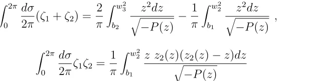
wi and the Neumann integrals of motion parametersba in terms ofJi and use (2.33). After finding a periodic solution of (2.30), this reduces to the problem of computing the two independent integrals on the r.h.s. of eqs. (2.38) and (2.39).
2.3
Moduli space of the multi-spin string solutions
We are thus interested in finding periodic finite-energy solitonic solutions of O(6) sigma model defined on a 2-cylinder that carry three global charges Ji. They can be parametrised by the three frequencieswi (orJi) as well by the two integrals of motion
ba. The five parameters (wi, ba) may be viewed as coordinates on a moduli space of these solitons.
Because of the closed string periodicity condition in σ, general solutions will be classified by two integer “winding number” parametersna which will be related towi and ba after solving the periodicity condition (2.21). In general, there will be several different solutions for given values of J1, J2, J3, i.e. the energy of the stringE will be
a function not only of J1, J2, J3 but also of the values of na.
the form of a round circle as in the two-spin and three-spin solutions of [1, 2] or a more general “bent circle” shape as in the three-spin solutions of Section 4 below.
Before turning to the S5 rotation case, it is useful to review how these different
string shapes appear in the case of a closed string rotating in flat R1,5 Minkowski
space. In orthogonal gauge, string coordinates are given by solutions of free 2-d wave equation, i.e. by combinations of ein(τ±σ), subject to the standard constraints
˙
X2+X′2 = 0, XX˙ ′ = 0. For a closed string rotating in the two orthogonal spatial
planes 12 and 34 and moving along the 5-th spatial direction we find (cf. (2.9))
X0 =κτ , X1+iX2 = x1(σ)eiw1τ , X3+iX4 = x2(σ)eiw2τ , X5 =p5τ , (2.40)
with
w1 =n1 , w2 =n2 , x1 =a1sin(n1σ), x2 =a2sin[n2(σ+σ0)]. (2.41)
Here σ0 is an arbitrary integration constant, and na are arbitrary integer numbers and the conformal gauge constraint implies that
κ2 =p25+n21a21+n22a22 . (2.42) Then the energy, the two spins and the 5-th component of the linear momentum are
E = κ
α′ , J1 =
n1a21
2α′ , J2 =
n2a22
2α′ , P5 =
p5
α′ , (2.43)
i.e.
E =
s
p2 5+
2
α′(n1J1+n2J2) . (2.44)
To get the two-spin states on the leading Regge trajectory (having minimal energy for given values of thetwo non-zero spins) one is to choose n1 =n2 = 1 with σ0 = π2.
The shape of the string depends on the values of σ0 and n1, n2. If σ0 is irrational
then the string always has a “circular” (loop-like) shape. In general, the “circular” string will not be lying in one plane, i.e. will have one or several bends. For rational values of σ0 the string can be either circular or folded, depending on the values of
n1, n2.
Consider as the first example the case of σ0 = 0. If n1 = n2 the string is folded
and straight, i.e. have no bends. Indeed, then X1+iX2 is proportional to X3+iX4
and thus one may put the string in a single 2-plane by a global O(4) rotation. If bothn1 and n2 are either even or odd and different then the string is folded and has
several bends (in the 13 and 24 planes). For example, if n2 = 3n1 then the folded
string is woundn1 times and has two bends (in this casex2 =x1(4x21−3)).
Next let us consider the case of σ0 = 2πn2. If n1 = n2 the string is an ellipsoid,
becoming a round circle in the special case of a1 =a2 [1]. The string is also circular
if n1 is even and n2 is odd. If, however, n1 is odd andn2 is even the string is folded.
For example, if n2 = 2n1 then the folded string is wound n1 times and has a single
The structure of the soliton string solutions in curvedS5case is analogous. Indeed,
the equations of motion of the Neumann system are linearized on the Jacobian of the hyperelliptic curve (2.36). The image of the string in the Jacobian whose real connected part is identified with the Liouville torus can wind around two non-trivial cycles with the winding numbers n1 and n2 respectively (see Appendix A).
Fig.1: Image of a physical string at fixed moment of time in the Jaco-bian (the Liouville torus). The string winds around the fundamental cycles with winding numbers n1 and n2.
The size and the shape of the Liouville torus are governed by the moduli (wi, ba). Specifying the winding numbers n1, n2, two of the five parameters (wi, ba) are then uniquely determined by the periodicity conditions. The actual shape of the physical string at fixed moment of time lying on two-sphere will depend on the numbersn1, n2
and on the remaining moduli parameters and may be of (bent) folded type or of circular type.
Let us now study the folded and circular string solutions in turn.
3
Folded string solutions
3.1
Folded bent strings with three spins
Our aim here will be to analyse folded string solutions of (2.30). We shall see that to have three non-zero spins the folded string must be bent at least at one point.
By definition, a folded closed string configuration is such that for all of the coor-dinates XM(σ, τ) = XM(2π−σ, τ), i.e. XM′ (0, τ) =XM′ (π, τ) = 0 (we choose σ =π as a middle point). In the case of our rotating ansatz (2.9) this leads to
xi(σ) = xi(2π−σ) , x′i(0) =x′i(π) = 0, i= 1,2,3. If x′
i vanishes for all i only at the two points, then the string has no bends. Such straight folded string can carry only one non-trivial component of the spin in flat space, but in the case of rotation in S5 it may carry two non-zero spins [4].
To analyse when the folded string can carry three non-zero spins let us use the angular (ψ, γ) parametrization of two-sphere formed by xi (2.22). Let us consider a folded string stretched alongγ and ψ,
−ψ0 ≤ψ(σ)≤ψ0 ,
π
2 −γ0 ≤γ(σ)≤
π
and assume that
ψ(π
2) =ψ( 3π
2 ) = 0 , ψ(0) =−ψ(π) =ψ0, ψ
′(0) = ψ′(π) = 0 , (3.2)
γ(π 2) =γ(
3π
2 ) =
π
2 , γ(0) =
π
2−γ0 , γ(π) =
π
2+γ0 , γ
′
(0) =γ′(π) = 0 .
(3.3) This configuration is a folded string without bends. The case with two spins consid-ered in [4] corresponds toγ0 = 0, so one may expect that to have a string with a small
non-zero J3 one needs to consider a case with small γ0. However, it is possible to see
that this no-bend case is not a genuine three-spin case – there is a global SO(3) rota-tion that can be used to eliminateJ3. Indeed, for a consistent semiclassical state
inter-pretation one has to check that only three components, J1 ≡J12, J2 ≡J34, J3 ≡J56
of the SO(6) angular momentum are nonvanishing. Assuming that the above string configuration exists when all the frequencies wi are different, the angular momentum conservation of J36 requires the vanishing of the following integral (cf. (2.22))
Z 2π
0 dσ x2(σ)x3(σ) =
Z 2π
0 dσ sinγ cosγ sinψ . (3.4)
However, it is easy to see that for the folded string configuration (3.3) the integrand here is positive for any value ofσ. ThusJ36(and alsoJ45) do not vanish. We conclude,
therefore, that for the case of allwi different, the above string solution does not exist. Now consider the case w2 = w3. As soon as w2 = w3, one can rotate the folded
string to place it entirely on the equator (γ = π2) of S2 inside S5. Then x
3(σ) = 0
and J3 = 0 for the transformed configuration. The conclusion is therefore that the
folded straight string configuration can only correspond to a two-spin case, i.e. the periodicity conditions should implyw3 =w2.
The reason why in the no-bend case one is able to rotate the string by a global SO(3) transformation to setγ = π
2 is that the folded string should be stretching along
a geodesic (i.e. some oblique big circle) of S2 (ψ, γ) part of S5. This follows from
the fact that both of the derivatives γ′ and ψ′ vanish only at the same (two ending)
points (σ= 0, π) of the folded string (having a wiggle or a bend at some intermediate point of the string would mean the vanishing of one of the derivatives ψ′ orγ′ there).
We conclude that to find a non-trivial folded string solution with three spins we need to admit a possibility of bends, i.e. the points on the string where one of the two coordinates has zero σ derivative while the other does not (see also Appendix D). For example, ifγ′ changes its sign not only at σ= 0, π but also at some 2n other
points while ψ′ does not that would mean one has n folds in γ but only one fold in
ψ, implying the existence of n bend points. In what follows we will be considering the simplest and most symmetric case of a single bend point located in the middle of the folded string, i.e. with γ′ vanishing at σ
0 = π2 and σ0 = 32π; such configuration is
expected to have minimal energy for given values of the three spins. To have a folded string with a single bend we will thus require
x′
i(0) =x′i(π) = 0 , x′3(
π
2) =x
′
3(
3π
In terms of the coordinatesζ1 and ζ2 in (2.25) these conditions can be satisfied if
ζ1(
π
2) =ζ1( 3π
2 ) =w
2
2 , ζ
′
1(
π
2) =ζ
′
1(
3π
2 ) = 0 . (3.5)
In view of equations (2.30) the second condition is equivalent to
ζ2(
π
2) =ζ2( 3π
2 ) =b2 . (3.6)
The conditions (3.5), (3.6) mean that there should exist 4 pointsσ1, ..., σ4 located as
0< σ1 <
π
2 ,
π
2 < σ2 < π , π < σ3 = 2π−σ2 < 3π
2 , 3π
2 < σ4 = 2π−σ1 <2π (3.7) at which ζ2 =w3, and x3 = 0. Passing through these points x3 changes its sign. The
exact positions ofσ1, ..., σ4 are determined by the values of the parameters wi and ba of the solution. Note that the middle of the folded string atσ = π
2, 3π
2 is not located
at x1 = 1, x2 =x3 = 0. Thus, at σ = 0 we have ζ1 =b1 and ζ2 = b2. Increasing σ,
bothζ1 and ζ2 increase until at σ=σ1 the coordinateζ2 reaches the point w23. Then
ζ′
2 changes its sign and ζ2 begins to decrease. At σ = π2 the coordinate ζ1 becomes
w2
2 and ζ2 reaches the turning point b2. Next, ζ1 begins to decrease and ζ2 begins to
increase until at σ =σ2 the coordinate ζ2 reaches the point w32 where ζ2′ changes its
sign again. After that both ζ1 and ζ2 decrease and at σ =π they reach the turning
points ζ1 =b1 and ζ2 =b2 (see Fig.2).
A
B
C D
x3
x1
x2
Fig.2: Bent string. The pointAcorresponds toσ= π2,32π, the pointB -toσ =σ1,2π−σ1and the points CandDare the turning points where
σ= 0 and σ=π. The turning pointsC and Dare symmetric w.r.t. to the plane 13. When b2 → w23 the bend point A tends to equator and
Thus, two derivatives ζ′
1 and ζ2′ are both positive on the interval 0 < σ < σ1, and
the equations of motion (2.30) take the form
dζ1
q
−P(ζ1)
= 2 dσ
ζ2−ζ1
, q dζ2
−P(ζ2)
= 2 dσ
ζ2−ζ1
. (3.8)
The periodicity conditions (2.21) follow from (3.8) and from the range (2.24), (2.35) of ζ1, ζ2 (these conditions do not depend on σ1)
Z w22
b1
dζ1(ζ2−ζ1)
q
−P(ζ1)
=π , 2
Z w23
b2
dζ2(ζ2−ζ1)
q
−P(ζ2)
=π . (3.9)
The presence of the coefficient 2 in the second equation reflects the fact that we are considering the single-bend solution. As a consequence of (2.30) we have also the following relation which is valid for any point σ from the interval 0≤σ≤2π
|dζ1
dζ2|
=
v u u t
P(ζ1)
P(ζ2)
. (3.10)
Then
Z w22
c1
dζ1
q
−P(ζ1)
=
Z w32
b2
dζ2
q
−P(ζ2)
, c1 ≡ζ1(σ1) , (3.11)
Z c1
b1
dζ1
q
−P(ζ1)
=
Z w32
b2
dζ2
q
−P(ζ2)
and, therefore,
2
Z w23
b2
dζ2
q
−P(ζ2)
=
Z w22
b1
dζ1
q
−P(ζ1)
. (3.12)
The conditions (3.9) and equations of motion for ζ1, ζ2 (3.8) also imply
2
Z w23
b2
ζ2dζ2
q
−P(ζ2)
−Z w
2 2
b1
ζ1dζ1
q
−P(ζ1)
=π (3.13)
It will be convenient for the analysis in next subsections to make the following change of variables ζ1,2 →ξ1,2
ζ1 =w22−(w22−b1)ξ1 , ζ2 =w23−(w32−b2)ξ2 , (3.14)
Then eqs. (2.30) take the form
dξ1
dσ !2
= 4w
2
21(b2−w22)
w2 32
ξ1(1−ξ1)(1−t1ξ1)(1−u1ξ1)(1−v1ξ1)
(1−u1ξ1−u2ξ2)2
, (3.15)
dξ2
dσ !2
= 4w
2
31(w32−b1)
w2 32
ξ2(1−ξ2)(1−t2ξ2)(1−u2ξ2)(1−v2ξ2)
(1−u1ξ1−u2ξ2)2
Here we introduced the parameters
t1 =
w2 2 −b1
w2 21
>0, u1 =−
w2 2−b1
w2 32
<0 , v1 =−
w2 2−b1
b2 −w22
<0 . (3.17)
t2 =
w2 3 −b2
w2 31
>0, u2 =
w2 3−b2
w2 32
>0 , v2 =
w2 3 −b2
w2 3 −b1
>0. (3.18)
3.2
System of equations for the leading correction to the
energy
Let us now concentrate on the case of solutions which have all three spins very large (1.1). The energy for such solutions is expected to scale as in (1.2). Our aim is to derive a closed system of equations which allows one to find the leading-order function
f1 in (1.2), thus determining the one-loop (first order in λ) correction to conformal
dimensions of the corresponding dual SYM operators with free-field theory dimension ∆0 =J1+J2+J3 in SU(4) irreps with Dynkin labels [J2−J3, J1−J2, J2+J3]. The
same system of equations should then be expected to emerge from the thermodynamic limit of the algebraic Bethe ansatz for the SO(6) spin chain derived from the SYM theory [19, 3, 21].
The two-spin case [4] and the relation (2.33) for the energy of the string suggest that one should look for solutions which have the following moduli parameters
wi2 =Jtot2 +ωi( Ji Jtot
) +O( 1 J2 tot
), ba=Jtot2 +βa( J i Jtot
) +O( 1 J2 tot
), (3.19) where
Jtot =
√
λ Jtot =
√
λ (J1+J2+J3) , (3.20)
is the total spin of the string. We shall assume that in the large Jtot limit the
“corrections” ωi and βa depend only on the ratios JJtoti =
Ji
Jtot. Note that the presence
of a linearO(Jtot) term inωi2andbain (3.19) can be ruled out by “parity” (wi→ −wi, etc.) considerations.
Then the relation (2.33) implies that
E2 =Jtot2 +λ(ω1+ω2+ω3−β1−β2) +O(
1
Jtot
), (3.21)
i.e.
E =Jtot+
λ Jtot
f1(
Ji
Jtot
) +O( 1
J3 tot
), f1 =
1
2(ω1+ω2+ω3−β1−β2) . (3.22) We want therefore to find the expressions for ωi and βa and thus for f1 in terms of
the current ratios Ji Jtot.
equations (2.37)-(2.38), and one of the equations (2.10) expressing spins through the parameters. This system can be written as follows in terms of the “hyperelliptic” integrals I10, I20,I11,I21,I22 defined in Appendix B
2I20 =I10 , (3.23)
2I21 =ω32I10+I11−π , (3.24)
ω1j1+ω2j2+ω3j3 = 0, ji ≡
Ji
Jtot
, (3.25)
ω1+ω2−ω3+
2
π 1
2ω
2
32I0 +ω32I11−
1
2(2I22− I12)
= 0, (3.26)
j3 =
2t2
π Z 1
0 dξ1
dσ dξ1
(1−u1ξ1) ξ2(ξ1) . (3.27)
Hereωij ≡ωi−ωj and
dσ dξ1
= √ω
32(1−u1ξ1−u2ξ2)
2qω21(β2−ω2)
1
q
ξ1(1−ξ1)(1−t1ξ1)(1−u1ξ1)(1−v1ξ1)
, (3.28)
which follows from eq.(3.8). We could use any of the other two equations in (2.10) instead of eq.(3.27).7 All of the parameters in (3.17),(3.18) and in the above system
of equations depend only on the ratiosji = JJtoti =
Ji Jtot.
Since the integral in (3.27) can not be computed analytically, there are at least two ways to proceed for a generic three-spin case. One may try to compute this integral and therefore to solve the whole system (3.23)–(3.27) numerically (see Section 3.4). One may also try to develop a perturbation theory around the two-spin solution of [4] assuming that the third spin componentJ3 is small as compared to the total spin
Jtot. Since the two-spin solution was expressed in terms of the elliptic functions, one
could expect that the same should be true for a perturbative expansion at the vicinity of the two-spin solution. This is indeed what happens as will be explained in the next subsection.
3.3
Two-spin solution and small
J
3expansion
As was mentioned above, the limit b2 → w32 should correspond to the two-spin
so-lution. In this case the folded string stretches along the equator, i.e. it is straight (without bends). This limit corresponds to a degeneration of the hyperelliptic curve (2.36) governing the string dynamics into an elliptic one.
To see explicitly how this happens let us change the variables ζ1,2 → ξ1,2 as in
(3.14). In the limit
ǫ≡w32−b2 →0
7Let us also note that we cannot use eq.(2.38) to determine the leading order correctionf
1because
one finds that t2, u2, v2 →0 and u1 →v1 so that eqs. (3.15), (3.16) simplify to
dξ1
dσ !2
= 4w212 ξ1(1−ξ1)(1−t1ξ1), (3.29)
dξ2
dσ !2
= 4w212 (1−u1)
1− t1
u1
ξ2(1−ξ2)
(1−u1ξ1)2
. (3.30)
Now one can recognize in eq.(3.29) the differential equation for the elliptic sn function, i.e. its solution is
ξ1 = sn2
K(t1)−
q w2
21σ, t1
. (3.31)
Here K denotes the complete elliptic integral of the first kind.8 In writing eq. (3.31)
we have also used the fact that ξ′
1 is negative on the interval 0 < σ < π2 and that
ξ1(0) = 1 due to the identity sn(K(t1), t1) = 1. Eq. (3.31) defines an elliptic curve
with modulus t1. Then the second equation (3.30) can be integrated to find ξ2. Note
that in the two-spin case the variableξ2 is an auxiliary one as the physical coordinates
x1, x2 (x3 = 0, γ = π2) are parametrized in terms of ξ1 only (cf. (2.25),(3.14)). The
simplicity of the two-spin case is thus related to the fact that the equations forζ1 and
ζ2 decouple whenb2 =w32.
To determine the parameters (t1, u1) entering eqs. (3.29) and (3.30) from the
periodicity conditions (3.12) and (3.13) let us study in more detail the relation (3.10). In general, the latter implies the following two equalities
I1(ζ1) =I2(ζ2) +I2(b2) , b1 ≤ζ1 ≤c1 , b2 ≤ζ2 ≤w23 , (3.32)
I1(ζ1) =−I2(ζ2) +I2(b2) , c1 ≤ζ1 ≤w22 , b2 ≤ζ2 ≤w32 , (3.33)
where we have introduced the two period integrals of the Abelian differential of the first kind:
I1(ζ1) =
Z w22
ζ1
dz q
−P(z) , I2(ζ2) =
Z w32
ζ2
dz q
−P(z) . (3.34) Making the change of integration variable z → w2
2 −(w22 −b1)ξ1z for I1, and z →
w2
3−(w23−b2)ξ2z forI2, and using (3.14) we obtain a more useful form ofI1, I2 given
in Appendix B. In the limit ǫ = w2
3 −b2 → 0 both integrals can be easily computed
and one finds
I1(ǫ→0) =
2Π[u1,arcsin√ξ1, t1]
q w2
21w322 (b2−w22)
, I2(ǫ→0) =
2 arcsin√ξ2
q w2
31w322 (w32−b1)
, (3.35)
where Π denotes the incomplete elliptic integral of the third kind. Now (3.32) allows one to solve forξ2 in terms of ξ1, namely
ξ2(ξ1) = cos2
"s
(1−u1)
1− t1
u1
Π(u1,arcsin
q ξ1, t1)
#
. (3.36)
Since ζa → ba implies that ξa → 1 we find the following transcendental equation relating the parametersu1 and t1:
Π(u1, t1) = π
s
u1
(1−u1)(u1−t1)
. (3.37)
Then eq. (3.36) can be written as
ξ2(ξ1) = cos2
"
πΠ(u1,arcsin
√
ξ1, t1)
Π(u1, t1)
#
, (3.38)
This relation is valid for all values ofξ2 from the interval [0,1]. In particular, one
rec-ognizes that ξ2(1) =ξ2(0) = 1 and ξ2(c1) = 0, where c1 ≈0.56862. This dependence
of ξ2 on ξ1 is a reflection of the U-shaped form of our string.
Let us now consider the periodicity condition (3.13):
2I21−I11=π (3.39)
where we have introduced the following period integrals of the other Abelian differ-ential of the first kind:
I11=
Z w22
b1
zdz q
−P(z) , I21=
Z w32
b2
zdz q
−P(z) . (3.40) The same change of variables as for (3.32) allows one to compute these integrals in the limit ǫ→0 with the result
πw2 3
q w2
31w322 (w32−b1)
− w
2 2
u1
q w2
21w432
h
pK(t1) + (u1−p)Π(u1, t1)
i
= π
2. (3.41)
where p= w22−b1
w2
2 >0. With the help of (3.37) the last equation reduces to
K(t1) =
π
2
q w2
21. (3.42)
Eqs. (3.37) and (3.42) completely determine the parameterst1, u1of the two-spin
solu-tion in terms of the frequenciesw1, w2. Note that the requirement ξ1(π2) =ξ1(32π) = 0
produces the same eq. (3.42) fort1.
In the limit ǫ→0 we can compute the integral
Z π2
0 (ζ1+ζ2)dσ=
1
2(2I22−I12), (3.43) where
I12=
Z w22
b1
z2dz
q
−P(z) , I22 =
Z w23
b2
z2dz
q
As a result,
Z π2
0 dσ (ζ1+ζ2) =
π
2(w
2
1+w23) +
q w2
21E(t1), (3.45)
where E is the complete elliptic integral of the second kind. Then in the limit ǫ→0 eqs. (2.37) and (2.38) reduce to the following equations
J1
w1
+ J2
w2
= 1, (3.46)
w1J1+w2J2−w22 =−
2
π q
w2
21E(t1) , (3.47)
with eq. (2.39) being their consequence. Summarizing, we have shown how the three-spin hyperelliptic solution degenerates to the two-three-spin elliptic one, the later being completely determined by the system (3.37), (3.42), (3.46) and (3.47). The energy of the two-spin solution is determined from
E2 =κ2 =w2
1 +w212 t1. (3.48)
In the two-spin case withJ1 =J2 ≡ J, J3 = 0 we know that [4]
t1 = 0.826115 +... , w1 = 2J −
0.272922
J , w2 = 2J +
0.272922
J . (3.49) We can then use (3.37) to determine w3. The result is
u1 =−0.777383 , w322 = 2.32025, w3 = 2J +
1.70597
2J . (3.50)
Finally, it is now easy to compute the energy of the three-spin string up to the term linear inj3 ≡ JJtot3 . To this end we should expand the system of equations (3.23)–(3.27)
inǫand use the two-spin solution as the zero-order approximation. Then this system reduces to a linear system which can be readily solved. We find that the parameters
ωi, β1, u1, t1 in (3.17), (3.19) have the following expansion in j3:
ǫ≡w23−b2 =ω3−β2 = 6.12528j3 , j3 ≡
J3
Jtot
(3.51)
u1 =−0.777383 + 0.424835j3 , t1 = 0.826115 + 0.183849j3 ,
ω1 =−1.09169−3.86759j3 , ω2 = 1.09169−2.95629j3 ,
ω3 = 3.41194−0.20351j3 , β1 =−0.712032−4.11054j3 .
Using these values of the parameters we find for the energy E2 =J2
tot+ω1+ω2−β1 +ǫ =Jtot2 + 0.712032 + 3.41194j3 , (3.52)
i.e.
E2 =Jtot2 + 0.712032λ+ 3.41194 J3
Jtot
Thus the energy has the form (1.6) with positive coefficients
E =Jtot+ 0.356016
λ Jtot
1 + 4.79183 J3
Jtot
. (3.54)
The coefficient f1(0) = 0.356016 is the same as in the two-spin solution [4],9 while
f1(1) = 4.79183 is the string-theory prediction for the term linear inJ3 in the one-loop
anomalous dimension of the dual CFT operator.
3.4
Comments on folded string solutions with general values
of
J
1, J
2, J
3Let us now study more general folded string solutions which can be far from the two-spin configuration. This can be done numerically as follows. One starts with three valuesw1, w2, w3as input parameters and solves the two periodicity conditions (3.12),
(3.13), for the unknownsb1 and b2. Then one determines the parameter c1 =ζ1(π/4)
by solving numerically eq.(3.12) (or, equivalently, eq.(3.11) ). With these values
w1, w2, w3, b1, b2, c1 one can then compute
Z 2π
0
dσ
2π(ζ1+ζ2) =
2
π Z w23
b2
z2dz
q
−P(z) − 1
π Z w22
b1
z2dz
q
−P(z) , (3.55)
Z 2π
0
dσ
2πζ1ζ2 =
1
π Z w22
b1
z z2(z)(z2(z)−z)dz
q
−P(z) (3.56)
and find J1, J2, J3 from eqs. (2.37)-(2.39). The parameters of different solutions
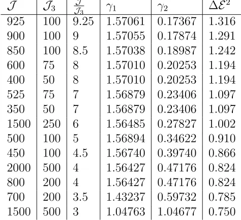
ob-tained in this way are shown in Table 1.
w2
1 w22 w32 b1 b2 c1 J1 J2 J3 ∆E2
23.52 25.80 28.29 23.87 27.81 24.70 2.20 2.32 0.48 1.06 34.65 36.89 39.40 35.01 39.00 35.82 2.75 2.86 0.38 0.94 47.63 49.88 52.40 47.99 51.97 48.80 3.21 3.32 0.47 0.96
1 4 9 1.14 4.64 2.31 0.26 0.59 1.33 3.45
[image:22.612.154.469.356.437.2]25 28 33 25.14 28.64 26.31 1.30 1.56 2.55 2.88 49 52 57 49.14 52.64 50.31 1.82 2.13 3.35 2.83 49 53 59 49.06 53.36 50.61 1.50 1.96 3.97 3.42 49 55 64 49.01 55.09 51.33 1.16 1.59 4.96 4.47 49 51 55 49.36 52.27 50.08 2.69 2.18 2.30 1.92 Table 1: Parameters for string configurations with different values of angular momenta.
9This coefficient has a simple origin: f(0)
1 =π12(2t−1)[K(t)]2, wheret= 0.826115 is the (unique)
The first three entries are cases close to the two-spin case, which are indeed con-sistent with eq.(3.53) for the energy. The input values of w1, w2, w3 are obtained
from eqs. (3.51) using J3 = 0.5, Jtot = 5 for the first entry, and J3 = 0.4, Jtot = 6,
J3 = 0.5, Jtot = 7, for the second and third entries. According to eq. (3.53), the
perturbation-theory values for the correction to the energy ∆E2 ≡E2 −J2
tot =λ∆E2
found in the expansion in powers of J3
Jtot are, respectively, ∆E
2 ∼= 1.04, ∆E2 ∼= 0.96,
∆E2 ∼= 0.94. They agree with the results in Table 1.
The values ofJ1, J2, J3 are also in good agreement with direct perturbation theory
results. Small differences are expected, in view of the higher order corrections in powers of J3
Jtot and in view of the fact thatJtot is not very large (the results of Table
1 represent summation of all terms in 1
Jtot expansion, while the (3.53) contains only
the leading correction term). Other cases in Table 1 are far from the two-spin case, i.e. have J3 of the same order as (or larger than) J1, J2.
In general, a random choice of w1, w2, w3 may not correspond to a folded string
solution. For large Ji, there are no folded string solutions when the w2
ij are not small compared to the w2
i.
We have considered some cases with the same values of w2
31, w212 , but increasing
values of wi. They exhibit the following interesting fact. The differences b1−w12 and
b2 −w22, c1 −w12 are always the same. The difference in the energy ∆E2 approaches
some asymptotic value as Ji increase.10 For the particular entries of Table 1, one observes that as the differences w2
i −w2j increase, b1 gets closer to w12 and b2 gets
closer tow2 2.
In conclusion, there exist folded string solutions for diverse values of J1, J2, J3.
In the case when J3 is smaller than J1, J2, the numerical calculation reproduces the
perturbation theory results of the previous subsection.
4
Three-spin string solutions of circular type
4.1
String solutions of circular type in ellipsoidal coordinates
Let us start with recalling that our parameters are assumed to satisfy in general the conditions (2.24),(2.35), i.e.
w12≤ζ1 ≤w22 ≤ζ2 ≤w32 , b1 ≤ζ1 ≤b2 ≤ζ2 . (4.1)
As was discussed in Section 3, to describe a folded string we should consider b1 lying
in the same range as ζ1, and b2 lying in the same range asζ2, i.e.
w12 ≤b1 ≤w22 , w22 ≤b2 ≤w23 . (4.2)
10For very large values ofJ
i the difference ∆E2≡E2−Jtot2 should depend only on the ratios
Ji
To find a “circular” string solution we should relax at least one of the conditions (4.2), i.e. to assume that eitherb1 orb2 do not belong to the corresponding intervals.
Thus there are two different cases to be considered
I. w12 < b2 < w22 , II. b1 < w12 .
Let us start with the caseI. We have then two options for the value of b1:
(i) w12< b1 < w22 , or (ii) b1 < w12 .
In what follows we shall consider the case (i), because the case (ii) appears to similar toII.
When w2
1 ≤b1 ≤w22, we have
b1 ≤ζ1 ≤b2 , w22 ≤ζ2 ≤w23
and there are many different circular string configurations with these values of pa-rameters. Let us first consider the simplest one corresponding to
b1 =b2 ≡b , i.e. ζ1 =b .
Making the change of variableζ2 →ξ2,
ζ2 =w23−w232ξ2 ,
we get from (2.30) the following equation forξ2
dξ2
dσ !2
= 4w312 ξ2(1−ξ2)(1−tξ2) , t≡
w2 32
w2 31
. (4.3)
Assuming the initial conditionξ2(0) = 0, the solution of this equation is
q
ξ2 = sn
q w2
31σ, t
. (4.4)
According to this formula the function √ξ2 oscillates between -1 and 1 as σ goes
around the string. Hence, if we want our solution to describe a circular type string with a winding number n, the real period of the function sn should be equal to
2π n
q w2
31, i.e.
2πqw2
31 = 4nK(t). (4.5)
this point let us write down the expressions for the physical-space coordinates xi in (2.25):
x1 =
v u u t
b−w2 1
w2 21
w231−w232ξ2 w2
31
1/2
, x2 =
v u u t
w2 2−b
w2 21
(1−ξ2)1/2, x3 =
v u u t
w2 3 −b
w2 31
ξ21/2.
When ξ2 changes from 0 to 1 allxi remain non-negative. However, x2, x3 can acquire
zero value, i.e. can reach the boundary of the coordinate patch xi ≥0 and, therefore, they may change sign. Change of the sign means that we go to another coordinate patch onS2. This is indeed the case as one can see by computing the derivativesx′
2,3:
One finds that x2 changes its sign when ξ2 crosses 1, while the sign of x3 changes
when ξ2 crosses zero. Thus, the shape of the resulting string configuration appears
to be of a circular type.
Conversely, for the folded string configurations of Section 3, the coordinate x3 is
zero, while x1 remains strictly positive as ξ1 changes from 0 to 1. We see once again
that the shape of the string depends essentially on the relation between the parameters of the moduli space (cf. Section 2.3) which explicitly occur in the expressions for the coordinates xi in terms of the variableξ2: xi =xi(ξ2;wi, ba).
It is useful to note that in the limit w3 → w2 the periodicity condition (4.5)
reduces tow2
31=n2 and thus we recover the circular three-spin solution found in [1]:
q
ξ2 → sn(nσ,0) = sinnσ . (4.6)
We want to emphasize that neither the solution (4.4) nor the periodicity condition (4.5) depend on b. This parameter occurs only in the expressions of xi through ξ2
and it tells us how many spins our solution has. For generic b we have a three-spin solution. A two-spin solution arises in the limit b → w2
1 (or b → w22). In this limit,
x1 = 0, i.e. J1 = 0, while
x2 =
q
1−ξ2, x3 =
q
ξ2. (4.7)
The spins J2 and J3 are then easy to compute
J2 = w2
Z 2π
0
dσ
2π(1−ξ2) = w2
t "
t−1 + E(t) K(t)
#
, (4.8)
J3 = w3
Z 2π
0
dσ
2πξ2 = w3
t "
1− E(t) K(t)
#
, (4.9)
where we made use of the explicit solution (4.4). These two equations can be used to express w2,3 through J2,3, while the parametert= w
2 32
w2
31 can be found from (4.5). The
energy is then given by
E2=w22+ w
2 32
We will not go here into the detailed analysis of the two-spin circular type solution above, we will do it in Section 5, where a comparison with the gauge theory results will be presented.
Let us consider now the limiting case whenw3 →w2. We also assume thatw12 < b1
and therefore b1 < ζ1 < b2. First we perform the following change of variables
ζ1 =b2−b21ξ1 , ζ2 =w32−w322 ξ2 , b21 ≡b2−b1 .
Then taking the limit w3 →w2 we get from (2.30) the following equations for ξ1, ξ2
dξ1
dσ !2
= 4hξ1(1−ξ1)(1−t1ξ1), (4.11)
dξ2
dσ !2
= 4h(1−u1)
1− t1
u1
ξ2(1−ξ2)
(1−u1ξ1)2
, (4.12)
where we introduced the parameters 0< t1 =
b21
b2−w21
<1, u1 =−
b21
w2 2−b2
<0, h=b2−w21 >0 . (4.13)
These equations have the same form as (3.29) and (3.30) governing the two-spin solutions for the folded string but there is an important difference. Now the variable
ξ2 enters the parametrization of the physical coordinates xi:
x21 = b2 −w
2 1
w2 21
(1−t1ξ1), x22 =
w2 2 −b2
w2 21
(1−u1ξ1)(1−ξ2),
x23 = w
2 2−b2
w2 21
(1−u1ξ1)ξ2. (4.14)
It is easy to see that the corresponding shape of the string is again of a circular type. As was pointed out in Section 2.3, generic winding string solitons are parametrized by two integers (n1, n2). To construct a corresponding solution we assume that the
variable √ξ1 oscillates between −1 and 1 with period 2nπ1
√
h. As above, this gives an equation that determines the parametert1:
K(t1) =
π
2n1
√
h . (4.15)
Then eq.(4.12) can be integrated to give
q
ξ2 = sin
h s
h(1−u1)
1− t1
u1
Z σ
0
dσ′
1−u1ξ1(σ′)
i
, (4.16)
where the initial condition ξ2(0) = 0 was assumed.
Suppose now that the variable√ξ2 performs n2 oscillations between −1 and 1 as
evaluated by a change of variables, and we obtain the second elliptic function equation to determine the parameteru1:
Π(u1, t1) =
π
2
n2
n1
s
u1
(1−u1)(u1−t1)
. (4.17)
Equations (4.15) and (4.17) generalize (3.42) and (3.37) for arbitrary winding numbers
n1 and n2. At this point it should be mentioned that imposition of the relation
w3 = w2 implies that the three spins Ji are not any more independent but rather satisfy an additional constraint. Indeed, our solution is governed by four parameters
w1, w2, b1, b2 which obey the five equations, three of them determine the spins Ji through these parameters and the other two are the periodicity conditions (4.15) and (4.17). Therefore, one of the equations is in fact a constraint forJi.
The case of the “round-circle” string can be recovered by taking first the limit
t1 →0 and then u1 →0. In this double limit eqs. (4.15) and (4.17) reduce to
b2 −w12 =n12, n1 =n2. (4.18)
Let us consider now the case II and show that it is quite similar to the case I. This time we have the following range of parameters
b1 ≤w21 < w22 < b2 < w32. (4.19)
and thus
w21 ≤ζ1 ≤w22, b2 ≤ζ2 ≤w32. (4.20)
To demonstrate that we are dealing with string solutions of circular type we consider the limit b2 →w32. Performing a change of variables
ζ1 =w12+w221ξ1 , ζ2 =w32−(w32−b2)ξ2 . (4.21)
and taking the limit b2 → w32 one obtains the same system of equations (4.11) and
(4.12) parametrised by
t1 =−
w2 21
w2 1 −b1
<0, u1 =
w2 21
w2 31
>0, h =w21−b1 >0. (4.22)
The coordinatesxi depend only on the variable ξ1
x1 =
q
ξ1, x2 =
q
1−ξ1, x3 = 0. (4.23)
Applying the same arguments as above we conclude that the form of the string is of a circular type.
4.2
String solutions of circular type in spherical coordinates
As was already discussed, when all the frequencies wi are different, the ellipsoidal coordinates allow one to separate the variables and formulate a closed system of equations that determines the energyE as a function of spins Ji. However, when two of the three frequencies coincide, the U(1) subgroup of O(3) in (2.1) is restored and it is useful to adopt the spherical coordinates. To make a contact with [1] in this and the following subsection we relabel x1 →x3, x3 →x2 and consider the case when
w1 =w2 > w3 . (4.24)
The spherical coordinates are global and thus particularly appropriate for the study of solutions with non-minimal energy that represent strings of circular type. Here we shall first present the equations for the spherical coordinates and then relate them to the above discussion of the circular type strings in the ellipsoidal coordinates. The equations of motion for the spherical coordinates ψ and γ follow from the action (2.1) and the metric (2.3), and in the casew1 =w2 take the form
(sin2γ ψ′)′ = 0, γ′′+1
2sin 2γ (w
2
13−ψ′2) = 0 . (4.25)
Then
ψ′ = c
sin2γ , c= const , (4.26)
γ′′
−c2 cosγ
sin3γ +
1 2w
2
13sin 2γ = 0 , (4.27)
and the conformal gauge constraint reduces to
γ′2 = κ2− c
2
sin2γ −w
2
1sin2γ−w23cos2γ . (4.28)
This can be rewritten as
x′2 =w2
13(x2 −a−)(a+−x2), x≡x3 = cosγ , (4.29)
where the constants a± are
a±=
1 2w2
13
h
w213+w21−κ2±q(κ2−w2
3)2−4c2w132
i
. (4.30)
Clearly, to have two different turning pointsa−anda+we have to impose a condition11
0 < a± ≤ 1. Note also that a+ = 1 for c = 0. The expressions of the integral of
motionc and the energy of the system in terms of the turning pointsa± are
c2 =w132 (1−a+)(1−a−), κ2 =w12+ (1−a−−a+)w132 . (4.31)
11This impliesw
To establish a connection with the discussion of the circular type strings in terms of the ellipsoidal coordinates, we introduce a new variable
ξ= x
2−a
−
a+−a−
.
Then eq. (4.29) takes the same form as (4.11) with parameters
h=a−w132 , t1 =−
a+−a−
a−
<0. (4.32)
As to eq. (4.26), we rewrite it as
ψ′2 = c2
(1−a−)2
1 (1−u1ξ)2
(4.33) with
0< u1 =
a+−a−
1−a−
<1. (4.34)
Using (4.31), one can establish a direct correspondence between eq. (4.33) and eq. (4.12). The periodicity conditions are then given by (4.15), where n1 = 1 and by
(4.17). In this way one recovers the ellipsoidal coordinate description of the circular type strings.
4.3
Energy of circular type strings
In this subsection we shall find numerical solutions of the periodicity conditions for the circular strings and calculate their energy in the spacial case of two equal frequencies (4.24).
Let us define the two “turning” angles γ1, γ2 by
a− = cos2γ1 , a+= cos2γ2 ,
so that
c=w13sinγ1sinγ2 , w13 =
q w2
1−w23 .
The string extends fromγ =γ1 (which is the value closer to the equator pointγ = π2)
toγ =γ2.
The string energy can be determined from
E2 =λκ2 =λ[w213(sin2γ2−cos2γ1) +w12] . (4.35)
Our aim is to express E as a function of J3 and J1+J2, i.e. of
J3 ≡
J3
√
λ , J ≡
J √
The parameters w1, w13 are given by
w1 = J
w3
w3− J3
, w13=w3
v u u
t J
2
(w3− J3)2 −
1 , (4.37)
so we have three unknowns w3, γ1, γ2 and three equations:
πw13=K1(γ1, γ2) ,
J3
√
λ =
w3
πw13
K2(γ1, γ2), nπ =K3(γ1, γ2), (4.38)
where K1(γ1, γ2), K2(γ1, γ2), K3(γ1, γ2) are the integrals which in the previous
sub-section where computed in terms of the elliptic functions,
K1(γ1, γ2) =
Z γ2
γ1
dγq sinγ
(cos2γ
2−cos2γ)(cos2γ−cos2γ1)
, (4.39)
K2(γ1, γ2) =
Z γ2
γ1
dγ sinγ cos
2γ
q
(cos2γ
2−cos2γ)(cos2γ−cos2γ1)
, (4.40)
K3(γ1, γ2) = sinγ1sinγ2
Z γ2
γ1
dγ (sinγ)
−1
q
(cos2γ
2−cos2γ)(cos2γ−cos2γ1)
. (4.41)
The system (4.38) can be reduced to a system of two equations and two unknowns
γ1, γ2 by noting that
J3
w3
= K2(γ1, γ2)
K1(γ1, γ2)
.
Using (4.37), the second and third equations of (4.38) become:
nπ =K3(γ1, γ2) , K2(γ1, γ2) =πJ3
v u u t
J2
J2 3[K
1(γ1,γ2)
K2(γ1,γ2)−1]
2 −1 (4.42)
These can be solved numerically for γ1, γ2. Note that for large J3 the square root
on the right hand side of the second equation must be very small. This gives a hint for the values of the parametersγ1, γ2 which solve these equations. We shall always
consider the case whenJ3,J≫1.
The general features which result from numerical analysis are the following. The above system has solutions for all possible n = 1,2,3, .... For given n, there is a minimal value of J3/J. A lower bound can be obtained for large n. For n ≫ 1, K3
must be large, which implies that the anglesγ1, γ2 are close to π2. In this region, one
can approximate the integrals, leading to the bound J3/J>1/4n2.
When J3/J is small, the solution has maximum eccentricity, withγ1 nearπ/2 and
γ2 near 0. As J3/J increases, the angle γ1 increases and γ2 decreases, until some