PERSPECTIVE
Eugene Levich
email:[email protected]
(Received 23 October 2009; accepted 31 March 2009)
Abstract
It is claimed that turbulence in fluids is inherently coher-ent phenomenon. The coherence shows up clearly as strongly correlated helicity fluctuations of opposite sign. The helic-ity fluctuations have cellular structure forming clusters that are actually observed as vorticity bands and coherent struc-tures in laboratory turbulence, direct numerical simulations and most obviously in atmospheric turbulence. The clusters are namedBCC- Beltrami Cellular Clusters - because of the observed nearly total alignment of the velocity and vorticity fields in each particular cell, and hence nearly maximal possi-ble helicity in each cell; although when averaged over all the cells the residual mean helicity in general is small and does not play active dynamical role. The Beltrami like fluctuations are short-lived and stabilize only in small and generally con-tiguous sub-domains that are tending to a (multi)fractal in the asymptotic limit of large Reynolds numbers,Re→ ∞. For the model of homogeneous isotropic turbulence the theory predicts the leading fractal dimension of BCCto be: DF = 2.5.This
−5/3 power law energy spectrum.
The most obvious role thatBCCplay dynamically is that the nonlinear interactions in them arerelatively reduced, due to strong spatial alignment between the velocity field v(r, t) and the vorticity field ω(r, t) =curlv(r, t),while the physical quantities typically best characterizing turbulence intermit-tency, such as entrophy, vorticity stretching and generation, and energy dissipation are maximized in and near them. The theory quantitatively relates the reduction of nonlinear inter-actions to the BCC fractal dimension DF and subsequent turbulenceintermittency.
It is further asserted thatBCCis a fundamental feature of all turbulent flows, e.g., wall bounded turbulent flows, atmo-spheric and oceanic flows, and their leading fractal dimension remains invariant and universal in these flows. In particu-lar, theoretical and numerical evidence is given indicating that
BCC in turbulent channel/pipe flows have the depth at the walls proportional to the square root of the Reynolds number in wall units, Ly ∝ √Re , which is equivalent to the frac-tal dimension in normal to the walls y direction DyF = 0,5,
and the total dimension DF = Dx,zF +DFy = 2 + 0.5 = 2.5.
Similar BCC structure and the same fractal dimension are suggested for geophysical turbulence, in near agreement with the recent comprehensive analysis of experimental and obser-vational data. It is asserted that the atmospheric and oceanic events, e.g., tropical hurricanes, tornadoes and other mesoscale phenomena, and probably ocean currents are manifestations of
BCCand their environs.
Generally BCC should be rather seen as the turbulence core, while the whole surrounding 3D flow as being created and sustained by the intense vorticity of BCC by means of induction, in a manner similar to that for an electric current generating magnetic field.
It is further argued that BCC is not only a theoretical concept important for fundamental grasp on turbulence, but may be a practical asset furnishing tools for turbulence man-agement in regular fluids and plasmas.
The concept of helical fluctuations in turbulence goes 25 years back in time, and while never totally abandoned nev-ertheless has been residing on the fringes of research activity.
ther validate or repudiate decisively the concept. However, re-cent large scale direct numerical simulations and proliferation of experimental and observational data showed convincingly how ubiquitous is the phenomenon of helicity fluctuations in various turbulent flows, from hurricanes and tornadoes to tur-bulent jets to solar wind plasma turbulence to turtur-bulent flows in compressible fluids. This allowed a fresh look at the concept and led to a quantitative theory exposed in this paper.
Foreword
Turbulence in ordinary fluids and plasmas is one of the most typ-ical phenomena found in observed Universe. Practtyp-ically all liquids, gases and plasmas are in a state of turbulent agitation. Still tur-bulence remains poorly understood after hundreds of years of most intensive study by thousands of researchers. Many have resigned to the fact and abandoned the spirited debate on turbulence nature that had been typical for the second half of the 20th century. Often turbulence is perceived, by laymen and professionals alike, as chaos. In reality turbulence is organized and coherent. This truly puzzling aspect of turbulence is disregarded by many in geophysical and me-teorological studies where sometimes phenomenological atmospheric models are built with only a remote reference to atmospheric turbu-lence organization. Far reaching predictions are made based on these models that have equally remote chances to come true.
Practitioners of turbulence in aeronautical engineering calculate the shapes and flight performances of aircrafts on a daily basis and fortunately do it successfully most of the time. As successful are me-chanical and civil engineers in other disciplines dealing with flows of fluids. They recognize the coherence of turbulence since they observe routinely the so-called coherent structures in turbulent flows around airfoils and in the pipes and all other flows important for engineering applications. Nevertheless, they may be not hard pressed to come up with fundamental explanation for this coherence. The truth is that the engineering community has accumulated during the hundreds of years of experience and especially since the advent of aeronautics so much empirical data and know-how on turbulent flows in thousands of situations. All these data and tremendous know-how are sum-marized today in semi-phenomenological equations, tables and more recently computer models and used by engineers with remarkable dexterity and ingenuity in a reliable manner in most of engineering applications. The contemporary engineers are like the architects of the antiquity who built not burdened by the knowledge of Newton’s laws and statics and did it magnificently.
need to have a degree in mechanical engineering, it may be even counterproductive, to notice that ocean dwellers and birds, propelling with amazing elegance through their (turbulent) habitat, have more profound understanding of turbulence management than we do. The attempts to emulate their techniques did not bring much success.
But it is when observing the atmospheric and oceanic turbulence, the planetary and mesoscale geophysical events, that the lack of un-derstanding is most apparent. On geophysical scales we are miniscule inside observers. Even the small size geophysical events are huge for us. We don’t have to peer inside trying to glimpse some small scale structures as we do in engineering scale turbulence. And here we encounter real enigmas.
The greatest one is the recurrent and obviously organized global planetary scale atmospheric and ocean flow patterns. Usually we take it for granted and do not enquire for the reasons. Many believe that meteorologists surely have the knowledge and explanations for this. In reality meteorologists know well how limited is the present understanding of the reasons for this organization. There is so much variability and chaos in every locality on Earth. Still on the global spatial and temporal scales the most basic flow patterns and sub-sequent weather patterns can be anticipated with great confidence. The recurrence in the global weather patterns goes on forever and we are used to it to such a degree that we don’t view this truly amazing fact with surprise. We know that there are currents in the oceans and jets in the atmosphere. They flow like rivers through the ocean and air for thousands of miles for eternity of time. Why do these currents and jets not mix up, diffuse into respectively the surrounding ocean and atmosphere as we would expect based on our intuition and every day experience? Why the tropical storms, largely the same in num-bers and with roughly the same intensity, are generated every year in tropical ocean regions and travel thousands of miles holding the shape and coherence to release their energy and content at about the same spots on the globe? What are tornadoes and why they strike with seasonal regularity in more or less the same regions on land?
made of fluid motion organized in some way, but as soon as we try to define quantitatively what is this that makes us to perceive them as such we fail. There is no adequate scientific language to serve and quantify the intuitive recognition of these coherent structures. For an honest observer not burdened with the years of study of mun-dane meteorological details the coherence of geophysical shapes and weather patterns, when they are considered on adequate space and temporal scales, is short of miraculous. This coherence co-exists with tremendous local variability in space and time. All meteorological modeling is ineffective when weather predictions are extended over a week time period. How is it that from all the chaos and local unpre-dictability of turbulent flows the tremendous global order of things in the atmosphere and oceans is created?
To understand the origins and mechanisms of global flow organi-zation is of truly great significance. If not for the atmospheric and oceanic turbulence coherence our very existence on Earth would have not been possible. It is necessary to recognize that hurricanes, torna-does, ocean and atmospheric currents and other magnificent geophys-ical events are most probably coherent manifestations of one global turbulence, rather than just local events caused by freak random co-incidences of atmospheric and oceanic or land conditions.a
walls in pipe and channel flows, the coherent structures are mostly observed and studied in laboratory conditions near the boundaries. Some experimentalists still continue linking CS to some ill understood and particular boundary effects, e.g., remains of instabilities in the incipient laminar flows, rather than intrinsic constituent elements of turbulence. With no mathematical description and no unifying phys-ical concept the study of CS remains narrow in scope and stagnant.
Yet other kind of turbulence, which is more often than not con-sidered quite separately from turbulence in neutral fluids, originates in plasma. In many manifestations the conducting plasma can be treated as a continuous media. In this approximation the plasma flows are described by a set of magnetohydrodynamic (MHD) equa-tions (see Appendix). All plasma flows in astrophysical and planetary conditions are intensely turbulent, would it be the solar wind or stars corona, pulsars or galaxies. It is plasma turbulence that left unful-filled the last 50 years of work on controlled fusion and left us without the subsequent inexhaustible source of green energy. With no funda-mental understanding of turbulence and its coherent manifestations there is no much hope gaining control over it in neutral fluids or in plasma.
Despite its intractable reputation a comprehensive and to a cer-tain extent predictable understanding of turbulence must be possible. True wealth of experimental data and numerical simulations leave no doubts that the flows of fluids, laminar and turbulent alike are adequately described by the (semi-phenomenological) Navier-Stokes equations.1 The turbulent flows patterns as complicated as they are
must be the solutions of the Navier-Stokes equations. Unfortunately the Navier-Stokes equations with the exception of few particular cases of laminar flows are analytically intractable. The attempts to apply the most sophisticated apparatus of mathematical physics developed in the last half century for other complex problems of physics, e.g., the field theories and phase transitions, all led to frustrating fiascos and only put smoke on the real issues. Much effort was spent by enthusiastic physicists and applied mathematicians trying to apply the perturbation theories, closure models and renormalization group
1At least for the so-called Newtonian fluids such as water, gases and most of
methods to the Navier-Stokes equations with no much success. At the same time the computational capabilities have been growing in the last 25 years. Presently it is possible to simulate turbulent flows with simple geometry and at the values of Reynolds numbers approaching the laboratory conditions, although still very far from what is typical in nature. The analysis of these simulations allows making confident and deep conclusions on the structure of turbulence.
A remarkable property of the Navier-Stokes equations is that when it is re-written in dimensionless variables it contains only one in-trinsic dimensionless parameter, the Reynolds number. The Reynolds number is defined as:
Re=νLL
ν , (0.1)
whereLa characteristic typical scale of the flow is,νL is the velocity
associated with this scale andν =µ/ρis kinematic viscosity of the fluid with density ρ. For almost all flows in nature the Reynolds numbers are very large, ranging from 104−108 in the laboratories and engineering to 1010−1012in geophysical phenomena and reaching fantastic values in astrophysics. 2. For certain critical values ofRe≥ Recriticalall laminar flows universally become unstable and seemingly
erratic. This erratic or turbulent fluid motion consists of very large number of velocity harmonics or degrees of freedom.3 Therefore it is
only natural that it looks chaotic. How a flow becomes turbulent from a smooth laminar one that is the problem of transition to turbulence has been to some extent understood on a basic level in the last half a century.b
Quite distinct from the problem of transition to turbulence there is a subject of developed turbulence. Developed turbulence is a some-what loosely defined subject. What is usually understood by oped turbulence is a complex multiscale flow pattern such as devel-ops when the Reynolds number is much bigger than its critical value
2To have a better feeling of the orders of magnitude let us estimate a typical
value ofRein the laboratory conditions for a pipe air flow: diameter of the pipe L= 0,3×102cm, νL= 103cm/sec, νair= 0,1cm/sec, andRe= 0,3×10⁶. For
water it would be even bigger by one order of magnitude since water is much denser andνwater≈0,1νair.
3It will be seen shortly that the number of degrees of freedom in homogeneous
isotropic model of turbulence is of orderRe9/4, a huge number for any realistic
for which the transition to turbulence occurs, i.e., Re>>Recritical.
With regard to developed turbulence it is customary to adopt the sta-tistical language of description. The acute variability of the seemingly chaotic turbulent velocity field and very large number of participat-ing coupled velocity harmonics, or degrees of freedom, in actual fact compels one to describe turbulence in statistical terms. Implied in the statistical description is the assumption that despite the sensitivity to initial conditions and consequent lack of dynamical predictability, the features typical for most nonlinear dynamic systems, nevertheless certain relevant quantities describing turbulent flows in a meaningful way, when obtained by averaging over a significant span of time, or over a large volume, or most generally over the ensemble of partic-ular space-time realizations that originate from many distinct initial conditions, should acquire the same stable values (Batchelor, 1953). The same is true for the coherent structures (CS). They have best meaning within the context of developed turbulence in the sense of stable features remaining after the averaging over many realizations of turbulent flows with similar boundary conditions but originating from different initial conditions.
It should be noted that if there has been genuine progress in the last decades in understanding of fundamental developed turbulence in fluids it came from direct numerical simulations (DNS) of the Navier-Stokes equations and from fascinating geophysical observations.4 On
the other hand physical experiment of the last decades carried out in well equipped laboratories furnished relatively negligible new insight into the fundamental structure of fluid turbulence.
In the recent large scale direct numerical simulations of turbu-lence in a cubic box with periodic boundary conditions (BigBox tur-bulence) mimicking the so-called homogeneous isotropic turbulence
4The DNS, i.e., numerical solutions projected on a discrete lattice pattern,
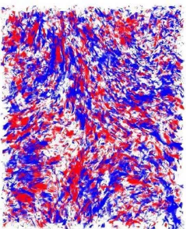
performed by Mininni, et.al. (2008a and 2008b), it was confirmed beyond reasonable doubt that clusters of stable Beltrami like helical structures of opposite signs of helicity shaped as thin and usually prolonged vortex structures, some stretching through much of the turbulent volume, is a universal feature of developed turbulence (see
Fig. 1). The clusters of helical structures having the opposite signs of helicity form the domains in the shape of intense vortex bands or filaments that are typical for all turbulent flows (seeFigs 2 and3). These domains are surrounded by the bulk of what appears as largely disorganized fluid motion.
In other recent works of Matthaeus, et.al. (2008a and 2008b), the authors experimented with numerically simulated plasma turbu-lence in magneto-hydrodynamic approximation (MHD). They found an anomalous distribution of angles of the plasma turbulent veloc-ity field v and plasma magnetic field B convected by the velocity field. Consistently the analysis of the solar wind data from satellite measurements showed similar alignment in the live as opposed to sim-ulated plasma turbulence. The authors point out that the alignment is similar to the alignment of velocity and vorticity that occurs in the Navier Stokes turbulence.5
Let us start from the Beltrami like helical structures and try to understand what is striking about their presence in turbulence. The Beltrami flows are defined as the flows where the velocity field vector is everywhere in parallel to its own vorticity, i.e., mathematically expressed as follows:
v·ω=v·[∇ ×v] =v·curlv (0.2)
The Beltrami flows are well known mathematical curiosities. They are exact solutions of the inviscid Euler equations describing inviscid (and in that unrealistic) flows, but having certain fascinating math-ematical properties that were exposed in the works of Arnold (1965,
5Solar wind is well conducting turbulent plasma blown from Sun. The
Figure 1: It is stated in Mininni, et. al. (2008a) that this is a zoom on a sample region of high vorticity in the flow. Turbulence in realizations is very inhomogeneous or intermittent in its structure and the regions of high vorticity occupy relatively small part of the total flow domain. Typical vortical structures, actually two merging vortical structures in the South-West corner, are sampled from this region with the velocity field lines drawn inside the structure in the upper image and near the structure in the image below. The authors claim that the velocity field lines are strongly helical aligning with the vorticity field lines.
1966 and 1974), but clearly understood by Moffatt (1985). In par-ticular, Beltrami flows have the maximal normalized helicity value for givenv and ω. c Helicity is a topological invariant, a particular consequence of the Kelvin’s conservation of circulation theorem in inviscid flows. In a simplified interpretation of all vortex lines closed helicity is a well known topological Hopf invariant, an integer measure of knottedness of divergence free solenoidal vector field lines and in this case vorticity field lines.6 But generally helicity is a continuous
for-invariant and more complex topological measure defined in a rigorous mathematical context in Arnold (1965 and 1966).
In the flows of real viscous fluids that are subject to the Navier-Stokes equations, for which neither energy nor helicity are invariant anymore because of the molecular scale viscous dissipation, still there are flows analogous to Beltrami flows which are the exact dynamical solutions. These are exponentially decaying with time Beltrami flows that relax asymptotically with time to the state of equilibrium still fluid at each point and therefore retaining in some sense the invariant topology of vortex lines, e.g., the normalized helicity (Libin, et.al., 1987; Libin, 2008).
How would such very particular and obviously coherent flow pat-terns in a well defined mathematical sense, preserving their distinct shape and topology appear in the midst of highly variable in space and time and seemingly disorganized fluid motion? Homogeneous isotropic turbulence is a pure turbulence model not contaminated by extraneous complications such as solid boundaries or complicated thermal sources typical for geophysical turbulence. As such it comes explicitly under the purveyance of the concepts first clearly expressed by Richardson in 1922 and culminating in the Kolmogorov theory of turbulence formulated in 1941, which since then has dominated the fundamental understanding of turbulence
The Kolmogorov theory postulates that the evolution of turbu-lence from any and all initial flow conditions is a statistical hierarchy of homogeneous isotropic and structureless eddies with progressively decreasing spatial scales randomly filling the whole fluid volume. The main feature of these eddies is a steady state constant flow of energy cascading from the larger scale eddies to the smaller ones with the smallest scale eddies benignly dissipating energy through molecular viscosity into heat. The main prediction of Kolmogorov theory, the
−5/3 power law energy spectrum for the turbulent velocity fluctua-tions as a function of inverse scale (or wavenumbers in Fourier space),
mally from the mapping of 3 - dimensional sphere into a 2 - dimensional sphere, S3 →S2. There is a family of invariants in higher dimensionsSn+1→Snand
has been approximately observed in great many experiments and geo-physical observations and therefore seems reasonably confirmed, even though there is still lack of confidence as regards the experimental accuracy.d But the large scale strongly anisotropic coherent helical
patterns have no place in Kolmogorov turbulence; they are in total contradiction with the usual wisdom that postulates that turbulence is made of volume filling structureless eddies.
To be more precise physical experiment, DNS in the last decades, and of course the atmospheric observations have been long time re-vealing that the distributions of small distance variations of the flow field velocity, vorticity, viscous energy dissipation and other related quantities7 are statistically inhomogeneous and strongly
non-Gauss-ian, in contrast with the velocity field at a point which is primarily determined by large scale motion and well approximated by the Gaus-sian law statistical distribution. It has been long known, e.g., Batch-elor and Townsend (1949) and BatchBatch-elor (1953) that the anomalously large, by comparison with the Gaussian statistical law values, vorti-cal activity and energy dissipation are situated in bands, filaments as they are often called, in relatively small flow sub-domains and temporal bursts of activity. This bunching together in small space sub-domains and short temporal bursts of intense activity of small scale dominated turbulent events is known as turbulence intermit-tency (see Section 5 below). This phenomenon gave rise to the phe-nomenological fractal models of turbulence, e.g., Kolmogorov (1962), Obukhov (1962), Novikov and Stewart (1964), Monin and Yaglom (1975), Mandelbrot (1974), Mandelbrot (1983), etc. These fractal models of turbulence as a rule saw intermittency as corrections to the Kolmogorov turbulence affecting high order statistical correla-tions but not undermining the basic tenets of the cascade theory.8
Intermittency is not a phenomenon found in turbulence alone. It
7That is essentially the quantities expressed via velocity field space and time
derivative
8In particular, fundamentally important for understanding the fractal strucure
is a feature typical of dynamical chaos originating in most nonlinear dissipative systems. But such endemic intermittency is of course a far cry from the spatially delineated helical coherent structures that are observed in the midst of turbulence so clearly and unambiguously. The coherent helical build-up of the intermittent bands of vortical activity in the midst of seemingly disorganized fluid motion, in a model that is closest in mimicking the conditions of homogeneous isotropic turbulence, shows that it is timely, in fact long overdue, to reassess both the Kolmogorov theory of turbulence and the still prevailing feeble interpretation of coherent structures in turbulence.
The observations of Beltrami like helical structures and related anomalies, made in Mininni,et.al.(2008a) and Mininni,et.al.(2008b), were largely predated and predicted in the works of previous decades. The theoretical concept of helical structures or fluctuations and their connection to the coherent structures (CS) on one hand and inter-mittency and fractals on the other, in turbulent flows irrespectively of their origin, was formulated in a series of works published over a period of time, e.g., Levich (1982), Levich and Tsinober (1983), Tsinober and Levich (1983), Levich and Tsinober (1984), Levich and Tzvetkov (1984 and 1985), Shtilman, et.al. (1985), Levich (1987), Levich and Shtilman (1988), Levich, et.al. (1991), Levich (1996). In these works the viewpoint was advanced that the coherent heli-cal fluctuations are the fundamental building blocks of all turbulent flows. The fluctuations are borne and die at multiple scales, as befits the general self-similarity and scaling conceptual foundation of tur-bulence theory, and on a fast time scale that tends to zero in the limit
Re→ ∞ in most of turbulent flow space. Because of this fast time scale the helicity fluctuations were called ’virtual’. The helical fluc-tuations are of both positive and negative helicity signs, clustering and screening each other, so that the global helicity in representative space/time domains remains small, but strictly speaking with mirror symmetry likely not respected.9
9Althoughh certain violation of global mirror symmetry was observed in DNS
In each of the virtual helical fluctuations the nonlinear coupling between the turbulent harmonics is somewhat reduced during their life time, while the vorticity and vorticity production attain increas-ing values at their boundaries. The volume occupied by the helical fluctuations decreases as most of them die out because of the short life span of helical correlations but eventually the fluctuations attain stability, or better to say a long enough life time span on a fractal sub-domain with the material volume tending to zero in the limit
Re→ ∞. But at the same time despite their small relative volume as compared with the total flow domain the helicity fluctuations and their environs contain most of turbulent activity.
The assumption of self similarity implies that while the volume occupied by the helical structures tends to zero in the limit Re → ∞, their total bounding surface area tends to infinity. The regions of decreased nonlinear coupling and on the contrary most intensive turbulent fields amplitudes, e.g., vorticity generation, overlap each other in this limit. In other words the helical structures and their boundaries together become a fractal set of dimension 2 < DF <3
embedded in the 3D fluid domain.
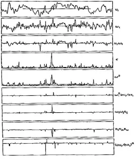
If the transient fluctuations and stable helical structures in thus defined sub-domains of flow realizations are indeed present than the first and simplest experiment would be to measure the distribution of angles betweenv and ω fields. The distribution is likely to show tendency for v and ω to be parallel or anti-parallel. Indeed, in the pioneering DNS of Shtilman, et.al. (1985), Pelz, et.al. (1985) and Pelz, et.al. (1986) such anomalous alignment of v and ω was ob-served as moderate size peaks in the probability distribution function
P df(cosθ) =P df(v·ω/|v||ω|) near the maximal and minimal values
cosθ= +1 and cosθ=−1. The peaks are natural to interpret as a contribution from the helical fractal set to the totalP df(v·ω/|v||ω|) in space/time realizations, but also as a relict trace from the transient helical fluctuations (see Fig. 4). This is why this ”anomaly” persists typically in representative sub-domains of turbulent flow, including the domains with low turbulent intensities.10
10The anomalous angle distribution was first numerically established at the very
Figure 4: From Farge, et. al. (2001) it shows theP df(v·ω/|v||ω|) =
P df(cosθ) in DNS of turbulence in a box with periodic boundary con-ditions. In this interesting DNS the authors using a mathematical method of wavelets sampled out what they call a coherent compo-nent of the velocity field in turbulent flow. This coherent compocompo-nent shows a quite distinct alignment of v and ω = curlv fields. The incoherent component shows no alignment. But apparently the to-tal velocity field shows similar alignment. What it means likely is that the regions of low vorticity typically retain certain coherence as well and can be seen as a relict trace of previously strongly coherent helicity fluctuations. The P dfresults are totally similar to the ones obtained in much earlier works of Shtilman, et. al. (1985) and Pelz, et. al. (1985).
It is likely that for similar reasons and to the same end there is an observed anomalous alignment between the velocity field and mag-netic field in turbulent plasma described in Matthaeus, et. al. (2008a and 2008b) for DNS of MHD turbulence and actual observations of real turbulence in solar wind (see Fig. 5 and Fig. 6). The authors reasonably asserted that the cross-helical patches similar to fluid tur-bulence helical clusters exist in plasma turtur-bulence as well, but with
substitution of vorticity by the magnetic field.
The reduction of non-linear coupling in the hierarchy of helical fluctuations is of great significance and allows in the long run turbu-lence in fluids as we see it in nature to exist (Levich, 1987; Shtilman and Polifke, 1989). It is the mechanism of intermittency and the rea-son for the relative stability of large scale vortical structures in the flows of fluids in nature. It was asserted in Levich (1987) that a spa-tially and temporally small active sub-domain formed by the hierar-chy of helical fluctuations generates the Kolmogorov spectrum. This assertion allowed calculating the reduction of the nonlinear coupling in the structures in this sub-domain and subsequently the fractal di-mension of this sub-domain. The calculation led toDF = 2.5 in the
limitRe→ ∞. Although the Kolmogorov energy spectrum is correct the mechanism that forms it is different from the one postulated in the Kolmogorov theory. Subsequent to the helical build-up of tur-bulence it was proposed in Levich (1980) and Levich (1987) that the interactions in turbulent flows are inherently non-local with the flow harmonics of widely disparate scales strongly interacting with each other. This is again contrary to the tenets of Kolmogorov theory, but strongly supported by the sited DNS.e
Somewhat similarly with the above concept Moffatt (1985) and Moffatt (1986) suggested that turbulence generally consists of un-stable/shortlived in space/time Beltrami blobs separated from each other by the surfaces of intensive dissipation. Moffatt (1984) also suggested that the Kolmogorov energy spectrum is formed not by the Kolmogorov mechanism, but via induction by a particular class of vortical spiral singularities embedded in turbulence midst. His analysis and classification of the unique properties of the Euler flows (stationary solutions of the ideal fluid Euler equations) and in par-ticular of Beltrami flows is imperative for understanding the helical concept of turbulence.
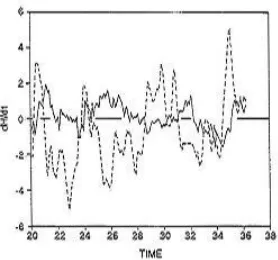
Figure 5: From Matthaeus, et. al. (2008a) it shows P df(v · B/|v||B|) = P df(cosθ) for DNS of MHD turbulence in a box with periodic boundary conditions. The different curves correspond to different runs with different initial and forcing conditions. The qual-itative similarity with Fig. 4 is pretty obvious.
Figure 6: The same as in the previous figure, but for satellite mea-surements over long time periods and different orientations in relation to the solar wind. It is clear that after averaging over all orientations the resulting figure would look strikingly similar to the one obtained from DNS (for instance combine away and towards sectors).
[image:20.420.139.271.241.339.2]cor-recting feature superimposed on Richardson-Kolmogorov turbulence structure, imagined as made of randomly dispersed and structure-less fluid eddies, they are rather the turbulence. And long life time stability of relatively large scale helical blobs bunched into small sub-domain is made possible by diminishing and balancing the nonlinear coupling in the Navier-Stokes equations that creates them and strives to destroy. Although the long-lived helical structures occupy only a vanishingly small fraction of the fluid space/time domain they cluster together like cells with opposite sign of helicity forming large patches of the most intensive events, e.g., coherent patches of vorticity and vorticity generation that are usually observed as CS. It is this do-main that is asserted to sustain the Kolmogorov energy spectrum and turbulence in general in the whole fluid domain.
It is almost trivial to add that the solid boundaries most actively facilitate the coherent helical structures birth and death, e.g., Levich (1996), since in general turbulence originates most readily and is most intensive in the boundary layer (BL) near the solid boundaries. The CS in BL turbulence are just the elongated domains of intense vor-ticity and it was conjectured that they are made of strongly helical cells of opposite sign of helicity, so that the total helicity is zero or small, but with reduced nonlinear coupling inside each cell providing relative stability to them and their environs. Equally they exist as elongated vortex bands in turbulence far away from boundaries and in turbulence created with maximal nearness to (statistically) homo-geneous and isotropic conditions, e.g., turbulence past a grid and in BigBox numerical turbulence as is clear from the cited works, and may be most importantly in atmospheric, oceanic and plasma turbu-lence. To avoid semantic ambiguity and intermittent choice of words patches, bands, or filaments, I suggest to call the coherent structures by what they really are - Beltrami cellular clusters -BCC.
The above assertions were in part made before. In what follows they will be reiterated and further quantitatively justified with con-fidence supported by accumulated experimental evidence.g
1
Basic Equations and Definitions
amazing phenomenon that science oriented audience of general pro-file deserves to be updated on progress in its understanding. This is why it is prudent to start from the beginning.
The basic equations governing the flows of incompressible viscous fluids are the Navier-Stokes equations:
Dv/Dt=∂tv+ (v· ∇)v==−∇P+ν∆v+F, (1.1)
or in index notations useful for anisotropic flows:
∂tvi=∂k(vivk+δikP) =ν∂k∂kvi+Fi (1.2)
In the Eqs. (1.1) - (1.2) P is pressure, Fi is an external body force
acting on the fluid assumed to be a divergence free (∇·F=∂iFi=0),
∂t=∂/∂t;∂i=∂/∂xi;∇2=∂i2=∆is the Laplacian operator,νis a
kinematic fluid viscosity, the densityρis set to unity and the fluid is assumed incompressible, so that the velocity field is divergence free:
∇ ·v=∂ivi=0. (1.3)
The quadratic nonlinear term in The Navier-Stokes equations consist of two parts. One is the inertial convection term from the general definition of the full derivative D/Dt =∂t+v· ∇, in the Eulerian
(field) representation of continuous media. 11 The other is the
obvi-ous pressure gradient force, which is in incompressible fluids not an independent field, but is determined from Eq. (1.3). This is clear by applying the divergence ∇ operator to the both sides of Eq. (1.1) with the result:
P =−∆−1∇ ·[(v· ∇)v]. (1.4)
Together with boundary conditions, for instance the usual for appli-cations no-slip boundary conditions at the solid surfaces bounding the flow:
vS(r,t) =0. (1.5)
The Eqs. (1.1) (1.4) in principle fully define the velocity field and pressure would it be laminar or turbulent flow.h If to set ν = 0, a
11In the Eulerian representation a fluid flows in relation to an observer so that
physically impossible situation that would correspond to the infinite molecular path length, than the Navier-Stokes equation becomes the Euler equations. The latter are the Newton equations for the contin-uous media driven by the pressure gradient moving in relation to an observer:
Dv/Dt=∂tv+v(∇ ·v) =−∇P. (1.6)
Also in this approximation, which is never true in reality, the non-slip boundary condition does not hold since there is no friction at the boundaries. Instead a less restrictive boundary condition is ap-propriate stating that the normal to the surface boundaries velocity component is zero should be used, i.e.,n·vS(r,t) =0.i
It is instructive to rewrite the Navier-Stokes equations in the so-called rotational form. Setting the non-fundamental forceF=0for the moment and using identical vector transformations the equivalent form for the Eq. (1.1) is as follows:
∂tv−[v×ω] =−∇(P+v2/2) +ν∆v, (1.7)
or in tensorial form:
∂tvi−iklvkϕωl=−∂k(P+vivk/2)δik+ν∆vi, (1.8)
because of the identity:
∂k(vivk)≡ −jklvkωl+δik∂k(vlvl)/2, (1.9)
where ω = [∇ ×v] = curlv, or in the components ωi = ikl∂kvl
is the vorticity field introduced in Foreword. Applying the curl =
∇×operator to both sides of Eq.(1.4) we obtain even more compact looking form of the Navier-Stokes equations:
∂tω−curl[v×ω] =ν∆ω, (1.10)
or in another useful form the Eq.(1.10) can be written as follows:
Dtω=∂tω+ (v·ω=−(ω· ∇)v+ν∆ω. (1.11)
In principle for a given vorticity field the velocity fieldv= (∇×)−1ω
integral expression similar to Bio-Savart relation between the mag-netic field and the current creating it, or the other way around.12
Therefore the Eq. (1.10) is a closed equation for the vorticity field. This way of rewriting the Navier-Stokes equation is important and revealing for understanding fluid dynamics. In the approximation of ideal fluidsν = 0 the equation forω becomes one from a wide class of dynamical equations for the so-called ”frozen-in” fields convected by a fluid motion. Frozen-in fields can be scalars, vectors, tensors or anything else that defines a field. In fluid mechanics the frozen-in fields are usually scalar and vector fields. If a frozen vector field line at zero time passes through a certain material fluid line belonging to a fluid element then for all other times it will pass through the same material line. The vector lines are rigidly attached to the fluid particles through which they pass. If the fluid elements are running away from each other, as they do in a turbulent (or any chaotic) flow then the corresponding frozen field lines will be stretched indefinitely to follow the motion of fluid particles. The nonlinear term in the left side of Eq. (1.11) is actually a passive convection of the field lines, while the nonlinear term on the right side of Eq. (1.11) is responsible for the stretching of the vector field line. If one considers a scalar field then the analogous equation of motion will have only a convection term left. For instance the dynamical equation for the heat transfer is:
∂tT+v· ∇)T=κ∆T, (1.12)
whereκis the molecular heat conduction coefficient. Whenκ= 0 Eq. (1.12) describes a passive scalar convection. Even such simplest sit-uation becomes very complicated when the velocity field is turbulent or merely a given random field (e.g., Falkovich and Fouxon, 2005).13
12One should not forget the potential part of the velocity field that should be
restored to have the imcompressibility condition∇ ·v=∂ivi=0fulfilled (e.g., Batchelor, 1979). In practical applications the solution of Eq. (1.6) and restora-tion of the potential part of the velocity field from the corresponding Laplace equation is difficult for most boundary conditions, except infinite media and peri-odic boundary conditions. Nevertheless, the fact that the vorticityωfield can be seen as creating the flowvfield is very significant for understanding turbulence.
13Convection of passive admixtures is a complex problem it nevertheless seems
An important and much more complex example is the magnetic field Bconvected by a flow of conducting plasma. If the plasma ve-locity is stationary than the whole set of MHD equations degenerates into a dynamical equation for the magnetic field and is as follows (see Appendix):
∂tB−curl[v×B] =η∆B, (1.13)
whereη is the electric conduction coefficient. Whenη is substituted by ν and B by ω the Eqs. Eqs. (1.13) and (1.10) are formally the same. When ν = η = 0, respectively in (1.10) and (1.13), the fields are frozen in the fluid and their lines move together with the material fluid elements to which they are attached at t = 0. There is a profound analogy between the kinematic properties of frozen-in vector fields. The study of frozen-in fields goes all the way back to the 19th century Kelvin’s theorem of conservation of circulation or what is the same the theorem of conservation of vorticity flux and similar theorem of conservation of magnetic flux. More recently there has been renewed interest to the frozen-in fields since their properties are closely connected to mathematical knots and other topologically invariant objects. With respect to fluid mechanics this subject was analyzed by Arnold (1965, 1966), but deeply understood and made clear by Moffatt (1985).
The dynamics of frozen-in fields is peculiar even for the simplest case of a scalar additive convected by a random velocity field. But for the vector fields it is extremely rich in results. For instance the dynamo effect, the exponential growth of magnetic field in moving conducting fluids, so important for the origin of magnetic field in astrophysics and elsewhere, is a result of this peculiar frozen-in dy-namics.14 In a random flow field the fluid particles generally ”run
away” from each other like in Brownian motion, so that the distance between any pair of them increases with time. In consequence the magnetic field lines stretch by these ”run away” fluid particles be-cause the lines are frozen into the fluid particles. The stretching of
e. g., the magnetic field, by turbulent velocity field (e. g., Moffat, 2001)
14In this case the flow field should not be necessarily the real turbulent flow
magnetic field lines is necessary (but not sufficient) condition for the growth of magnetic field.j The terms in (1.11) and (1.13) responsible
for the field lines stretching are −(ω· ∇)v and −(H· ∇)v, respec-tively forω andHfield lines.
The difference between Eq. (1.13) and Eq. (1.10) is that the mag-netic field is convected by a given fluid motion, so that Eq. (1.13) is quasi-linear, but the vorticity field is thecurlof the velocity field and hence Eq. (1.10) is fundamentally nonlinear. In fact for a given dis-tribution of vorticity the velocity field can be determined everywhere by means of induction from an integral relation similar to Bio-Savart induction law relating current and the magnetic field it generates (e.g., Batchelor, 2000). In other words the vorticity field can be seen as a principal one generating the flow field such that the vortex lines are frozen in this flow in ideal fluids. In real turbulent motion the fluid particles also ”run away” from each other, so that the distance between each two initially closely adjacent fluid particles grows expo-nentially with time for short times before the nonlinearity effects take hold. The vortex lines are stretched by this run away motion since they are frozen into the fluid particles. This stretching of vortex lines results in the rapid growth of vorticity amplitude and is generally be-lieved to be the basic mechanism of developed turbulence formation in fluids. Despite the differences the kinematic similarities between the MHD and the Navier-Stokes equations have profound method-ological implications for the theory of turbulence and therefore I will discuss this analogy and the implications below.
in the limitRe→ ∞, the flow properties should becomeRe indepen-dent, i.e., universal as long as the boundaries and geometry remain the same or their influence can be disregarded. Of course this does not mean that one can just omit the viscous term in Navier-Stokes equations and use the ideal fluid description. The limitRe → ∞is not at all the same asν= 0. Because the viscous term is the higher derivative term and there are always such small scale spatial varia-tions of the turbulent velocity field when it becomes dominant. This may be a trivial comment that nevertheless is important to bear in mind. From the outset it should be noted that it is not at all granted that the universal limit Re → ∞ exists. Or it may exist for some velocity related quantities and not to exist for others. In any event it is instructive to rewrite the Navier-Stokes equations in dimensionless units as follows:
Xi=xi/L;Vi=vi/vL;P0=P/vL2;τ=νt/L
2. (1.14)
Then the Eqs. (1.1) are as follows:
∂τVi+Re∂k(ViVk+δikP0) =∂k2Vi. (1.15)
The Eqs. (1.1) can be also rewritten in a different way such that theRe−1factor stands in front of the viscous second space derivative term in the r.h.s. of the Navier-Stokes equations. But the way it is written in (1.15) is more suitable for the further exposition.15
There are (at least) three quantities that are especially important for the theory of turbulence: energy (per unit mass), helicity and vorticity. Let us start from the energy per unit mass (it is reminded that the fluid density is set to unity,ρ= 1). Multiplying Eq.(1.2) by
vi and integrating over the fluid volume one finds after some simple
rearrangements (i= 1,2,3 and∂k=∂/∂xk):
∂tE=∂t
Z
vj2/2dV =
I
[vk(vi2/2 +P)−2νvieik]dSk+
−2ν
Z
e2ikdV +
Z
viFidV , (1.16)
15In what follows we shall alternate dimensionless and dimensional units
where the integrand of the surface integral is the energy flux:
jkE=vk(1/2v2i +P)−2νvieik, (1.17)
whereeikis the stress (or deformation) tensor typical for continuous
media:
eik= 1/2(∂kvi+∂ivk). (1.18)
The remaining two terms on the r.h.s. of Eq. (1.16) are the energy increasing due to the work done by the body forceFand the energy decreasing due to dissipation by viscous forces. If the surface is a solid boundary, at which v = 0 the surface integral vanishes, the nonlinear coupling term naturally conserves energy, and one is left with the energy acquisition due to the external force balanced by the dissipation terms. If one sets both dissipation and the force zero than the Eq. (1.16) is the obvious energy conservation law in inviscid fluids. The local viscous dissipation rate per unit volume per unit time is hence:
(r,t) =−2ν(eik)2=−ν/2(∂kvi+∂ivk)2. (1.19)
Apart from energy a quantity fundamental for turbulence description is a quadratic scalar measure of vorticity intensity-entrophy Λ =ω2.
One can derive from Eq.(1.11) the following balance equation:
Z
∂tΛ/2dV =
Z
ω·(ω· ∇)v−ν
Z
[∇ ×ω]dV. (1.20)
In (1.20) the integration is assumed over the infinite volume or a compact flow domain. In a steady state it follows then:
Z
ω·(ω· ∇)vdV=
Z
ωiωk∇kvidV >0. (1.21)
trivial vector manipulations that the viscous dissipation term in the balance equation (1.16) can be rewritten in the following identical way:
−2ν
Z
e2ikdV =− Z
ω2dV. (1.22)
This is an important relation showing that as enstrophy grows si-multaneously the global energy viscous dissipation does (note that of course 2e2
ik6=ω2locally).
Helicity is another peculiar invariant of the inviscid Euler equa-tions. Let us introduce helicity density pseudo-scalar product h =
v·ω and helicityH as follows:
H =
Z
hdV =
Z
v·ωdV. (1.23)
Then a simple calculation shows that:
∂tH =∂t
Z
hdV ==∂t
Z
v·ωdV=
=
I
[ωk(1/2v2−P)−vkh]dSk−2ν
Z
ωiijl∂jωldV , (1.24)
( ωiijl∂jωl = ω·curlω, ijl is the absolutely anti-symmetric unit
tensor). The integrand in Eq.(1.24) is the helicity flux similar to the energy flux (1.17):
jkH=ωk(1/2vi2−P)−vkh. (1.25)
If the integration is over a compact domain Dbounded by a vor-ticity surface∂D such that the normal to the surface vorticity com-ponent is zero,ωn|∂D= 0, in particular over infinite flow domain, the
surface integral vanishes and consequently helicity is the exact invari-ant of the Euler equations, as energy is. Helicity is a pseudo-scalar and can be positive or negative.16 The same is true for the viscous term in Eq. (1.24). In difference to the energy and vorticity balance equations the viscosity can be either a sink of helicity or a source.
16Solid boundaries at which of courseω·n|
Helicity is non-zero only for the flows lacking the reflectional (mirror) symmetry and as was mentioned above is a topological invariant.17
Briefly helicity is usually interpreted as a measure of knottedness of divergence free solenoidal vector field lines, and in this case the vortex lines: helicity is proportional to the number of knots and link-ages made by the vortex lines. The helicity then would be a discrete quantity akin to topological Hopf invariant. In fact a more general interpretation of helicity as a continuous topological invariant mea-sure was analyzed by Arnold. The vortex lines in a compact fluid domain can be closed, knotted or not, or end at the boundaries. But they may have a non-trivial topology, e.g., winding about surfaces of arbitrary complexity (for non-differentiabler velocity flow field), or ergodically filling a fluid sub-domain without end.k In the ergodic
configurations the vortex lines can form asymptotically close linkages and knots and in general possess arbitrarily complex topology that remain topologically invariant under smooth (but not necessarily in-vertible) mappings induced by fluid motion.
Helicity is a particular topological invariant of flows of inviscid flu-ids. However helicity is not the only invariant defining the topology of divergence free vector fields. It is easy to construct a vector field configuration that has zero helicity but is topologically complex and knotted, a usually demonstrated simple example being the Boromean ring, e.g., Moffatt (1969). In general there exists an infinite family of topological invariants for frozen-in fields more nonlinear than he-licity as was shown in Tur and Yanovsky (1993). They are all the consequences of the Kelvin’s theorem of conservation of circulation in inviscid fluids. It is however the connection between the helicity density and the nonlinear term in the Navier-Stokes equation that makes suggestive the role that helicity may play in turbulence: max-imal helicity in a compact flow domain or sub-domain is given by Beltrami flows yielding zero to the nonlinear coupling term in the Navier-Stokes equations.
Note that the viscous term in the balance equation (1.24) is not necessarily a dissipative one, meaning that it does not necessarily decrease |H|. The viscosity can reduce the absolute value helicity or generate it. As helicity is not positively defined so νω·curlω is
17Analogous to helicity invariant for Eq.(1.13) is cross helicityA=R
not. Generally there is no need for external helical forces to create a non-zero helicity in a turbulent flow. Although quite obvious this property results in surprising consequences for turbulence structure.
2
Kolmogorov Theory of Homogeneous
Isotropic Turbulence (K41): Part 1
The Kolmogorov theory of homogeneous isotropic turbulence-HIT-has been dominant for over half a century among the scientists seek-ing fundamental understandseek-ing of turbulence. The Kolmogorov the-ory is an important subject of geophysical studies. Many geophysi-cists view turbulence from a fundamental view point may be because they are best exposed to its many grandiose manifestations. On the other hand practitioners of turbulence in civil engineering and aero-nautics who are mainly concerned with turbulence near to the solid boundaries, highly anisotropic boundary layer (BL) turbulence, usu-ally have very limited use for the Kolomogorov theory, some of them viewing it as may be correct but for a highly idealized model that is not relevant for real life applications. Turbulent BL flows are full of structures. Although these structures were not given real mathe-matical description they are clearly visualized, so that the engineers are convinced that they are all important in their contribution to the physical parameters important for applications, e.g., heat and mass transfer, turbulent friction (drag) at the boundaries, etc. There are no such structures in the Kolmogorov model of turbulence. Thereby follows the usual and liely false argument that CS is the intrinsic feature of specifically BL turbulence.
On the other hand the celebrated prediction of Kolmpogorov the-ory, the−5/3 power law for the energy spectrum is observed in lab-oratory experiments modeling HIT, e.g., decaying turbulence past a grid and in part in geophysical phenomena, albeit with modifications and degree of uncertainty.l This law is to some extent confirmed in DNS, the Reynolds numbers are not high enough for confidence. The most surprising thing about this spectrum is that it is observed even in conditions remote from HIT such as for instance in large scale and highly anisotropic atmospheric flows.
it has become almost an Aristotelian must. It is very difficult to make even a slightest dent in its basic postulates. Because of this and for immediate reference by readers it is useful to remind here briefly the main tenets of the theory even though it has been done in thousands of papers before in dozens of different ways. From the outset it is necessary to state that although some of the basic principles of Kol-mogorov theory will be asserted wrong here the KolKol-mogorov energy spectrum will remain intact. However the physics behind the spec-trum is quite different from the one postulated in the Kolmogorov theory or implied by it. The Kolmogorov theory is often portrayed as a simple scaling relation for the flow energy spectrum, i.e., the distri-bution of energy of turbulent motion among different scales of motion, the velocity harmonics. But in actual fact the theory is very com-plex logically, although the mathematics is indeed simple. It relies on deep intuition into the nature of the Navier-Stokes equations which while cannot be solved still can be analyzed to some, admittedly lim-ited, degree and furnish indications to at least certain features and properties of turbulent motion. Such analysis of the Navier-Stokes equation had been carried out by generations of scientists and engi-neers for over a half century prior to Kolmogorov contribution and surely played role in the formation of the Kolmogorov theory of 1941. The Kolmogorov basic concept of 1941, often called K41, starts from the preceding poetic observation of Richardson made quite ear-lier in 1922 that rhymes ostensibly like this:
Big whorls have little whorls, Which feed on their velocity; And little whorls have lesser whorls, And so on to viscosity (In the molecular sense)18
Laminar flows are driven by extraneous forces, like pressure gra-dient in pipe flows. The mechanism for the laminar flow to become turbulent is, as was emphasized above, a distinct scientific problem beyond the scope of this paper. The fact is that laminar flows are almost always unstable. The simplest way to obtain turbulence is to stir fluid in a semi- random way. Imagine a paddle stirring fluid in
18This rhyme is quoted and misquoted by many. It carries such clear and
a large pail. Obviously this paddle can create a whorl or a vortex of the size comparable or bigger than the size of the paddle. This prime vortex size will be denoted as the integral scaleL. So far the motion is laminar. But the prime vortex or vortices are totally unstable and decompose into smaller vortices customary called eddies. And these eddies will decompose into smaller eddies and then into even smaller eddies and so forth till such time when eddies become small enough so that the viscous term in the Navier-Stokes equations becomes dom-inant, it is recalled that it is the second order space derivative of the velocity field, and these smallest viscous scale ld << L eddies
dissipate their motion into heat. Obviously the number of ld scale
eddies is much larger than the integral scale L eddies, since the to-tal incompressible fluid volume remains constant. The whole process can be likened to a cascade of water through the many steps in some waterfalls before sinking in a water reservoir below. But in this case the energy cascades through the eddies not in physical space but in the space of scales filling the same fluid domain.
The external forces are opposed by the internal viscosity friction of fluids and if there are boundaries by their friction at the boundaries In order for a steady state to set it should be that the same amount of energy as is injected into fluid by the stirring paddle to generate integral scale eddies is dissipated into heat by the many more small viscous scale eddies: the viscous forces balance the external forces so that the work done by the external forces is equal to the energy dissipated by the viscous forces.
The basic postulate of Kolmogorov theory is that the instabilities of integral scale laminar flow give rise to progressively smaller scales motion. As in the picture of Richardson the big eddy generates pro-gressively smaller and smaller eddies. The reason and possibility for eddies splitting into ever smaller eddies lies in the nonlinear nature of the Navier-Stokes equations for the velocity field. The simple mathe-matical details are discussed below in the next Section, but it is quite clear that when the Eqs. (1.1) - (1.3) are rewritten in Fourier space for the velocity field harmonics v(k,t) as a function of wave vectors
k:
v(k,t) = (2π)−1
Z
v(r,t)e−ik·rdV. (2.1)
harmon-ics, v(k), v(q) and v(k−q) or the triads of eddies in the space of scales and therefore generates in general different triadic scales of fluid motion. But still it is a non-trivial assumption in the spirit of Richardson that the generated scales of the velocity harmonics are predominantly smaller than the prime characteristic scale of fluid motion that is called the integral scaleL. The integral scale can be associated with an external body force acting on the flow, or with a leading scale of natural instabilities of the incipient laminar flow, e.g., caused by interaction with boundaries. But in principle the non-linear interactions could have created the opposite process to cascade, the growth of eddies, or what is usual to call the inverse cascade. How-ever, most probably as a rule the inverse cascade does not realize in 3Dworld.19
The next fundamental postulate of Kolmogorov is that in the limit of highReand after many cascade steps the small scale eddies of tur-bulence are universal, isotropic and homogeneous. That is to say that a turbulent motion that ensues from the initial integral scale motion, at the scales l << Lbecome self similar and universal. Therefore it
19In 2Dworld on the contrary the inverse cascade would be a reality and eddies
should be independent of the prime flow integral scale Land ofRe. The independence of Land ofRe signifies that the motion at these scales is totally dominated by the local in wavenumbers nonlinear couplings. Let us comment that the assumption that only local non-linear coupling remains would indicate that somehow the non-non-linear term in Eqs. (1.1) - (1.3), which generally describes all the inter-actions would reduce in some rigorous mathematical analysis of the Navier-Stokes equation, if such was possible. Some of the interac-tions, the non-local ones, would cancel out and only the harmonics with the local triads, such that all the three wavenumbers |k|,|q|
and|k−q|are the same order of magnitude, would remain. This is an important postulate of locality of interactions in Fourier space to bear in mind.
On the other hand by the nature of Eq. (1.1) there are some relatively small viscous scales of order ofld at which the linear
vis-cous term in Eq. (1.1), since it is the second order velocity field space derivative, would necessarily become dominant for any given arbitrary large value of Re. When eddies become so small the vis-cous friction just dissipates their motion into heat.20 Also, the
uni-versality naturally implies isotropy and homogeneity of small scale eddies in the inertial range after many steps of cascade, since there is no singled out scale in the inertial range to associate with either anisotropy, or inhomogeneity. This is the essence of the Kolmogorov HIT model. For consistency let us remind briefly the statistical math-ematical frame of this model.
The values of all turbulent fields are extremely variable in space and time and therefore it is natural to consider v(r,t) as a random function superimposed on the mean flow velocity, including the case of zero mean velocity. If the turbulent velocity were, indeed, a random field it would be fully characterized by the probability density:
W{v}Dv=W{v(N)}d(N)v(N)=
=limN→∞W{v(r1,t1),v(r2,t2), ...,v(rN,tN)}dv1v2....dvN,
(2.2)
20The energy spectrum is usually assuemd to be exponentially decaying in the
Z
W{v}Dv= 1,
where the functional W{v} gives the probability of having certain velocity field space/time 4D = (3 + 1) realization, at all the points in space and at all times, in the multidimensional functional space of all possible realizations.
If homogeneity and steady state of the velocity field are assumed, as befits HIT model, then the turbulent flow can be described by means of the velocity correlation functions of different orders at all points and all times, i.e., by all correlation functions of the type:
<v(r1,t1), ...v(rN,tN)>=<v(0,0), ...v(rN−1,tN−1)>=
=
Z
ΠN,Mi=1 v(ri, ti)W{v}Dv. (2.3)
In principle the knowledge of all the 1,2, ...N,1,2, ...M space/time correlation functions, if they exist and are finite in the limit ofN, M→ ∞would be equivalent to the full knowledge ofv(r,t).
In real experiments the ergodic assumption is applied and the ensemble averaging is understood in reduced sense as the time aver-aging over the values ofv(r,t) at a point. This is because practically all measurements can be made only at one, or at best few points in order to calculate the velocity derivatives, in a fluid flow. In numer-ical simulations even further approximation is usually accepted. If the space-time lattice on which the discretizedv(r,t) is calculated is dense enough, than the space and time averaging over the grid points is assumed to be sufficient for accurate calculations of the real en-semble averaged correlation functions. Even if one space realization of turbulence is represented by large enough N it is enough to cal-culate the space average for certain quantities. This is what is done usually in DNS for the models of decaying turbulence. In this model turbulence is triggered att0 by injection of energy into flow and then
allowed to evolve in time as it follows the Navier-Stokes dynamics. In real DNS even now the number of grid points is still too limited for calculating high order correlation functions. Moreover since some of the basic quantities, enstrophy and its generation rate for instance, are determined by relatively small subsets of grid points.
reduces to a nearly Gaussian distribution function. ButW{v}Dvis a strongly non-Gaussian functional for space-time variations of velocity at two or more points or its space derivatives related quantities, such as stress tensoreik, vorticityω, etc. This deviation from the normal
Gaussian law is associated with the phenomenon of intermittency.21
But let us go back to the Kolmogorov theory that does not concern itself with intermittency.
The velocity of the largest eddies vL is comparable to the total
variation of velocity ∆vLseparated by the distanceLthat is the scale
of the whole flow. ActuallyvL is smaller by a factor of two or three
but it does not matter really because ifRe= ∆VLL/v >>1 for the
whole flow it follows that:
v0l0>>1, (2.4)
where l0 is the size of the biggest eddies and byv0 ≈vL we rather
understand the root mean square of the fluctuating velocity typical; for the ensemble of proto-eddies, that ispv2
0.
The pro-eddies are the energy containing in the sense that they hold the major part of the energy associated with the total fluctuating part of the velocity, i.e., E ≈ v20. Successively the smaller eddies
are characterized by successively smaller, but still large Reynolds numbers and contain less energy,
Re>>Rei =v(i)li/v >Rei+1>>1, (2.5)
for each generation of eddies i. To avoid confusion it should be stressed that the notion of eddies is not really well defined. It would be safe to see the velocities v(i) as a characteristic fluctuating
ve-locity variance over a distance li, rather than the velocities of well
delineated vortices. In fact the latter can be seen as the definition of eddies. Eventually the size and the corresponding eddies velocity become small enough so that:
Red=vdld/v≈1, (2.6)
So that at these scales the dissipative term in the Navier-Stokes equa-tions becomes of the order as the nonlinear coupling. The scales of
21in Laboratory conditions the decaying turbulence is realized in turbulent flows
order ofldare called thedissipation range, while the scales from the
interval:
L≈l0>> ld, (2.7)
this range is called theinertial range. For each scalelilet us introduce
the time scale:
∆ti =li/v(i), (2.8)
during which the eddy is likely to decompose into smaller ones. The characteristic time ∆t0 >>∆ti is called (large)eddy turnover time.
During the time comparable with the eddy turnover time the proto-eddies will decompose enough, as the result of nonlinear interactions, so that the inertial range is formed and the dissipation range is reached.22
It should be taken into account that in real conditions there is always present a mean inhomogeneous flow with velocity|U(r,t)|>
∆vL. It is quite clear that for the assumption of homogeneity and
isotropy of eddies (in the statistical sense) it is necessary that the following condition is fulfilled:
|∂kUi|−1>>∆t0>>∆ti, (2.9)
so that it is clear that the assumptions of HIT can be understood only locally in globally inhomogeneous flow and are applicable only to eddies from the inertial range.
Assume that turbulence in the inertial range is in a steady state. It is a safe assumption provided that the considered time interval sat-isfies (2.9). Then it should be from the balance of energy requirement that the average energy fluxper unit volume per secpassing through the successive generations of eddies with velocities vi remains
con-stant. Or more correctly the ensemble averaged energy flux density
< >= const. Clearly the flux is in the space of scales li
dimin-ishing with the growth of generations of eddies i, or in the Fourier space of wavenumberski≈li. In physical space there is no
system-atic ensemble averaged flux in HIT. Since the dimension of< >is
length2×time−3(it is reminded that the densityρ= 1) from purely
dimensional considerations it follows:
< >≈∆v3L/l0≈v30/l0=...=v(3i)/li. (2.10)
22In DNS of decaying turbulence it is usually safe to wait for a few ∆t 0 to
Let us introduce a very useful quantity called eddy viscosity:23
veddy≈∆vLl0≈v0l0;vi,eddy=v(i)li. (2.11)
Then it follows:
< >≈veddy(v(i)/li)2=v(vd/ld)2 (2.12)
Note that the eddy viscosity is scale dependent and in general class of flows space-time dependent. The eddy viscosity can be also intro-duced as follows:
< >≈< (l0)>≈ −veddy <{∂kevi(l0) +∂ivek(l0)}2>≈ −2v < e2ik>,
(2.13) where ˜vi(l0) and < ˜(l0) > are the smoothed over the small scales
mean velocity field and dissipation rate respectively that are now dependent on the large scale−l0structure only and the differentiation
is done accordingly over these large scales. What the relation (2.13) means is a simple statement that as much energy is passed over from large scale eddies to the smaller ones caused by the stress at the large scales will be eventually dissipated by the molecular viscosity.
Now we can find again from purely dimensional considerations the eddy velocity as a function of their size. Since neitherRe norLcan enter by the assumptions of HIT it follows unambiguously:
v(i)=< >1/3l 1/3
i , (2.14)
providing an explicit law for the distribution of velocity fluctuations in turbulence as a function of their scale. The definition ofvi (2.14)
makes the relation (2.12) an identity. The corresponding character-istic Kolmogorov eddy numberiturnover time is:
∆ti≈li/v(i)=< >−1/3l2/3. (2.15)
A very important relation connectsLandld as follows:
L/ld≈(v0l0/v)3/4≡Re3/4. (2.16)
23The eddy viscosity is called like this because if the eddy size and velocityl
i, vi
are substituted by the molecular free path and velocityλf ree, vmolone obtains
The relation (2.16) furnishes self consistency to the definition of the inertial range, throughRe and this is what it should be because Re
is the only intrinsic parameter in the Navier-Stokes equation. The Eqs. (2.14) - (2.16) constitute the essential basis of the Kol-mogorov theory. It is amazingly simple and allows the calculation of most quantities that are needed for practical applications (Monin and Yaglom). Rarely in the history of science were such profound conclusions made on the basis of so few assumptions, which seem all quite innocuous and even obvious, and with such little mathemati-cal complexity. The generality of the results is also puzzling, since they are universally applicable for all turbulent flows, in pipes, at-mosphere, geophysics, oceanography, wherever one is concerned with flows far enough from the boundaries.24
It is practically more convenient, although not really more funda-mental to consider the Kolmogorov theory in Fourier space. Let us introduce the energy spectrum as follows:
E(k) =k2
Z
E(k)dΩ= (4π)k2(2π)−3(1/2)
Z
<v(0)·v(r)e−ikrdV
≡(1/π)k2
Z
<v(0)·v(r)>(sinkr)/krr2dr, (2.17)
where dΩ is the solid angle differential. The average energy density is now:
< E >=
Z
E(k)dk= 1/2< vi2(0,0)> . (2.18)
Now one applies to the spectrumE(k) the Kolmogorov assumptions in a slightly different manner. From the general dimensional consid-erations it follows:
E(k) =A < >2/3k−5/3φ1(Reφ2(kL). (2.19)
In the limit Re → ∞ we can expect universality and Re indepen-dence. This fixesφ1= 1. The postulated independence of the energy
spectrum from the large scale motions fixes φ2 = 1. So the
Kol-mogorov spectrum that will be called also the K41 spectrum in what follows becomes:
E(k) =A < >2/3k−5/3, (2.20)
24The distance from the boundaries is meant in dimesionless units defined by