scroll down to view the document itself. Please refer to the repository record for this item and our policy information available from the repository home page for further information.
Author(s):Dodds, Stephen J.
Title:Settling time formulae for the design of control systems with linear closed loop dynamics
Year of publication:2008
Citation: Dodds, S.J. (2008) ‘Settling time formulae for the design of control systems with linear closed loop dynamics’ Proceedings of Advances in Computing and Technology, (AC&T) The School of Computing and Technology 3rd Annual Conference, University of East London, pp.31-39
Link to published version:
SETTLING TIME FORMULAE FOR THE DESIGN OF
CONTROL SYSTEMS WITH LINEAR CLOSED LOOP
DYNAMICS
S J Dodds
Control Research Group[email protected]; [email protected]
Abstract: Two settling time formulae are numerically derived with the 5% and 2% criteria for the
step responses of control systems having linear closed loop dynamics that may be designed by the method of pole assignment to have multiple closed loop poles. The formula is shown to be accurate for closed loop systems of up to tenth order. To clarify the use of the formulae, model based and robust control system designs are carried out for a high precision vacuum air bearing application and experimental results presented.
1. Introduction
It is well known that the classical approach to control system design is based in the frequency domain with the assumption of linear plant dynamics and for single input, single input plants is a linear controller which is either one of several variations on the proportional integral derivative (PID) theme or a compensator. This approach is well documented in text books and has been established in industry for many years. Its evolution, however, has been influenced greatly by the constraints of practicable and economical hardware implementation of the past, the first versions being specially tailored analogue electronic circuits implemented with discrete components, the active components initially being thermionic valves, later replaced by transistors and more recently operational amplifiers. Such circuits are now being replaced by digital processors such as microcontrollers, field programmable gate arrays (FPGA) and digital signal processors (DSP), which are specially designed for fast execution of relatively heavy computational loads. The cost of control hardware is now drastically reduced by the software implementation of specific
system order is greater than 2, often 3 and not infrequently extending to 6. Occasionally, much higher orders are encountered in applications such as active vibration control and for this reason, systems up to 20th order are considered. Linear control theory is well understood and therefore the design of a control system is made relatively simple if a control technique is used that renders the closed loop system linear. This paper is restricted to single input, single output plants but a similar approach may be taken for the control of multivariable plants. The design approach presented here is a simple ‘top-down’ one in which the starting point is the desired performance in terms of the settling time with zero overshoot in the step response. It is important to note that if control energy is an important factor, then the settling time can be adjusted to minimise this within the constraint of maximum allowable settling time, attention also being paid to robustness (external disturbance rejection and insensitivity to plant modelling errors). It will be assumed here that the sampling time of the digital processor is sufficiently small compared with the time constants and modal periods of the open and closed loop system for continuous control theory to be applicable. The methods presented here are, however, extendable to discrete control theory.
A non-overshooting step response is a good starting point in the time domain for most control system designs and this can be achieved if the closed loop system has coincident negative real poles, according to the transfer function:
( ) ( )
n
c r
1 y s
1 sT y s
= +
(1.1)
where y is the measured and controlled output, y is the reference input, and r T is c the closed-loop time constant, i.e., the time
constant of each of the n first order systems which when connected in a chain will yield the desired nth order closed loop dynamics. Note that the usual unity d.c. gain is assumed but this can be made different if required. It is important to note that a controller must be used containing at least n adjustable parameters that can be set to realise the desired closed loop dynamics defined by (1.1). The flexibility of modern digital implementation renders this possible for all controllable plants.
2. Derivation of Formulae
2.1. Formulation of the problem
Let y be the steady state response to a step ss reference input. Then the settling time according to the x% criterion is defined as the time taken for yss−y(t) , to reduce to and thereafter remain less than x% of its maximum value. Traditionally x is chosen as 2 or 5 and therefore only these criteria are considered in this paper.
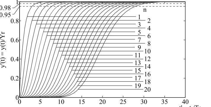
Fig. 2.1 shows a family of step responses of the closed loop system defined by (1.1) for orders ranging between 1 and 20. The step reference input is y (t) Y h(t)r = r , where
h(t) is the Heaviside unit step function. The outputs are normalised with respect to
r
Y , i.e., y′( )t =y( )t Yr and the time is normalised with respect to T , i.e., c t′ =t Tc.
0 5 10 15 20 25 30 35 40 0 0.2 0.4 0.6 0.8
t' = t /Tc
[image:4.595.131.487.97.278.2]y' (t) = y(t )/Y r n 1 3 5 7 9 11 13 15 17 19 2 4 6 8 10 12 14 16 18 20 0.98 0.95
Fig. 2.1: Family of normalised step responses of linear closed loop system with multiple poles.
The mathematical formulation of the problem of deriving such a formula is as follows. It may be shown that the general expression of the step response of the closed loop system defined by (1.1) is:
i n 1 c r c i 0 t
1 t T
y(t) Y 1 e
i! T − = − = −
∑
(2.1)which may be written as follows in terms of the normalised quantities already defined:
( )
n 1 i
i 0
1 t
y (t) 1 t e
i! − = − ′ ′ = − ′
∑
(2.2)The normalised settling time for the x% criterion would therefore satisfy
(
)
n 1 i sx% sx% sx% i 0 1 Ty (T ) 1 T e
i! − = − ′ ′ ′ = − ′
∑
andsince x 100=
[
1 y (T− ′ ′sx%)]
, then(
)
n 1 i sx% sx% i 0 1 T0.01x T e
i! − = ′ − ′
=
∑
(2.3)The exact settling time formula would be given by the closed form solution to (2.3):
(
)
(
)
sx% sx% c
T′ =f n, x ⇒T = f n, x T (2.4)
The exact function, f n, x , however, has not
(
)
yet been discovered, but section 2.2 provides a practicable approximation.2.2. A numerical solution
Observation of Fig. 2.1 reveals that the differences between the settling times of the responses of systems differing in order by 1 are nearly equal, so a linear approximation to the function, f n, x is possible for
(
)
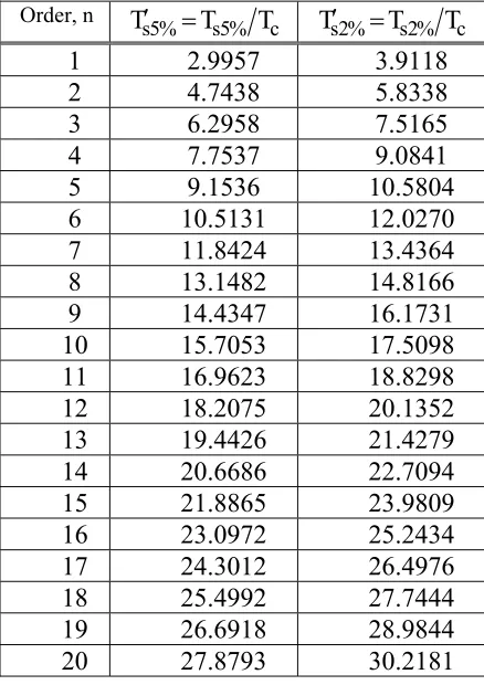
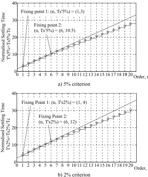
x 2 and 5= . For this purpose, the normalised settling times have been precisely computed for n 1, 2, , 20= K using a Matlab Simulink variable step simulation and Table 2.1 shows the results. These are plotted in Fig. 2.2 (a) and (b) for x 5= and x 2= , respectively. The question now arises of the choice of the linear approximation method and how many points to take. The classical approach would be to use all 20 points and apply a least squares fit.
Table 2.1: Normalised settling times of linear closed loop system with multiple poles.
Order, n
s5% s5% c
T′ =T T Ts2%′ =Ts2% cT
1 2.9957 3.9118 2 4.7438 5.8338 3 6.2958 7.5165 4 7.7537 9.0841 5 9.1536 10.5804 6 10.5131 12.0270 7 11.8424 13.4364 8 13.1482 14.8166 9 14.4347 16.1731 10 15.7053 17.5098 11 16.9623 18.8298 12 18.2075 20.1352 13 19.4426 21.4279 14 20.6686 22.7094 15 21.8865 23.9809 16 23.0972 25.2434 17 24.3012 26.4976 18 25.4992 27.7444 19 26.6918 28.9844 20 27.8793 30.2181 to obtain better approximations for these than would be obtained by using all the points. With reference to Table 2.1, the formula should fit the well known result of Ts5% =2.9957Tc ≅3Tc for n 1= , so the point
[
n, Ts5%]
=[1,3] should be one point on the straight line fit for x 5= . It may also be observed that for n 1= ,s2% c c
T =3.9118T ≅4T . This approximation is not quite as accurate as that for x 5= , but is chosen to yield a simple formula so the point
[
n, Ts2%]
=[1, 4] will be chosen for x 2= . Asreasoned in section 1, a practical approach would be to consider points up to n 6= and observation of Table 2.1 reveals two more points through which the straight line approximations can pass that should yield simple formulae. Thus, for n 6= ,
s5% c
T =10.5131T ≅10.5Tc yielding the point
[
n,Ts5%]
=[6,10.5] and Ts2%=12.0270Tc c12T
≅ yielding the point
[
n,Ts2%]
=[6,12].The straight line fit
sx% x x
T′ =C +M n (2.5)
where C and x M are constants to be x determined will be applied to the aforementioned fixing points in section 2.3.
2.3. The 5% settling time formula
Using the fixing points of Figure 2.2 (a) yields:
{
C M 3{
5M 7.5 M 3 2 C 6M 10.5++ == ⇒ C 3 M 3 2= −= ⇒= = ⇒( )
s5%
T′ =3 1 n+ 2. The settling time formula for the 5% criterion is therefore as follows:
( )
s 3 c
T = 2 1 n+ T or Ts=1.5(1 n)T+ c (2.6)
2.4. The 2% settling time formula
Using the fixing points of Figure 2.2 (b) yields:
{
M C 4{
5M 8 M 8 5 6M C 12+ =+ = ⇒ C 4 M 12 5= −= ⇒= = ⇒( )
s2% 4
T 3 2n
5
′ = + . The settling time formula
for the 2% criterion is therefore as follows:
( )
s 4 c
T = 5 3 2n+ T or Ts =1.6(1.5 n)T+ c
(2.7)
3. Accuracy Assessment
The settling times, T , obtained using nominal s settling times, Ts nom, in (2.6) and (2.7) were accurately determined by means of variable step Matlab-Simulink simulations.
0 1 2 3 4 5 6 7 8 91011 12 13 141516 17 18 191920 0
10 20 30
Order, n
Nor
m
alis
ed
S
ett
ling T
ime
T
's
5%
=
T
s5
%
/T
c
Fixing point 1: (n, Ts'5%) = (1,3)
Fixing point 2: (n, Ts'5%) = (6, 10.5)
a) 5% criterion
0 1 2 3 4 5 6 7 8 9 1011 12 13 141516 17 18 1920 0
10 20 30 40
Order, n
Nor
m
alis
ed Settling T
ime
T
's
2%
=
T
s2%
/T
c
Fixing Point 1: (n, T's2%) = (1, 4)
Fixing Point 2: (n, T's2%) = (6, 12)
[image:6.595.146.449.88.451.2]b) 2% criterion
Fig. 2.2: Normalised settling times and straight line fits
For n 1,2, ,10= K , the errors are within ±5%. This is considered acceptable for most control system designs, as illustrated by the families of step responses in Fig. 2.3, which all pass nearly through the point for which t T= s. If higher accuracy is required, however, then if the measured settling time is Ts m, then a ‘single iteration’ correction could be made by simply setting T to a new value: c
(
snom sm)
cnew T T c
T = T (2.8)
where Ts nom is the required settling time. Alternatively, Table 2.1 could be used to yield the value of T needed to realise the specified c value of Tsx%, x 2 or 5= , and this applies to
all system orders. According to Table 3.1, even for n 20= , the actual settling time, T , s would be approximately 12% less than the specified one, Tnom, using (2.6) or (2.7) and the correct settling time could still be realised by adjusting T as described above. c
4. Control System Design Examples
4.1 The plant
the position measurement, y, coming from a high resolution encoder.
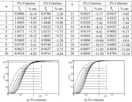
Table 3.1: Normalised settling times and % errors
5% Criterion 2% Criterion 5% Criterion 2% Criterion n
s
T% % err. T%s % err.
n
s
T% % err. T%s % err.
1 0.9986 −0.14 0.9780 −2.20 11 0.9423 −5.77 0.9415 −5.85 2 1.0542 +5.42 1.0418 +4.18 12 0.9337 −6.63 0.9322 −6.78 3 1.0493 +4.93 1.0440 +4.40 13 0.9258 −7.42 0.9236 −7.64 4 1.0338 +3.38 1.0323 +3.23 14 0.9186 −8.14 0.9157 −8.43 5 1.0171 +1.71 1.0173 +1.71 15 0.9119 −8.81 0.9083 −9.17 6 1.0012 +0.12 1.0022 +0.22 16 0.9058 −9.42 0.9015 −9.85 7 0.9869 −1.31 0.9880 −1.20 17 0.9000 −10.00 0.8951 −10.9 8 0.9739 −2.61 0.9748 −2.52 18 0.8947 −10.53 0.8892 −11.08 9 0.9623 −3.77 0.9627 −3.73 19 0.8897 −11.03 0.8836 −11.64 10 0.9518 −4.82 0.9516 −4.84 20 0.8850 −11.50 0.8784 −12.16
0 0.5 1 1.5 2
0 0.2 0.4 0.6 0.8 1
t/Ts
y/
Y
r
n 1 2 3 4 5 6 7 8 9 0.95
0 0.5 1 1.5 2
0 0.2 0.4 0.6 0.8 1
t/Ts
Y/
Yr
n 1 2 3 4 5 6 7 8 9 0.98
[image:7.595.73.527.124.475.2]a) 5% criterion b) 2% criterion
Fig. 2.3: Normalised step responses for multiple pole placement using the settling time formulae.
The plant equations are:
a m
x f M ,f= =K u, y K x= ⇒ =y bu
&& && (4.1)
where b K K= a m M. The slider mass, actuator constant and measurement constant are, respectively, M 3.25kg= ,Ka =0.8 A / V and Km =11.1 N / A.
The application of the settling time formulae in the design of a high precision motion control system for the rig will now be demonstrated, using pole placement first for a cascade IPD controller and then for a sliding mode controller (SMC), ref., Utkin (1992), with a boundary layer and an integral outer loop to remove steady-state errors due to disturbance forces.
4.2 The desired characteristic polynomials
In every case, application of the settling time formulae (2.6) and (2.7) to the desired closed loop transfer function (1.1) yields:
( )
( ) ( ) ( )
n n
s s
r
1 1
y s 2T or 5T
1 s 1 s
y s 3 4 3 2n
1 n
a) 5% criterion b) 2% criterion
= + +
+ +
1442443 144424443
(4.2)
( ) n ( ) n
s s
31 n 4 3 2n
s or s
2T 5T
a) 5% criterion b) 2% criterion
+ + + +
1442443 1442443 (4.3)
[image:8.595.74.286.131.310.2]4.2 Design of the IPD cascade controller
Fig. 4.1: IPD position control system
The closed loop characteristic polynomial is 3
s (s)∆ , where (s)∆ is the determinant of Mason’s formula applied to Fig. 4.1:
3 I
d p
2
b K
s 1 K s K
s s −− + + = 3 2
d p I
s +bK s +bK s bK+ (4.4)
For n 3= , (4.3) yields: 3
3 2
2 3
s s s s
6 18 108 216
s s s s
T T T T
+ = + + +
(4.5)
for the 5% criterion and 3
3 2
2 3
s s s s
36 108 1296 46656
s s s s
5T 5T 25T 125T
+
= + + +
(4.6)
for the 2% criterion. Comparing (4.4) with (4.5) and (4.6) in turn yields the required controller gains for the chosen criterion:
5% 5% 5%
d p 2 I 3
s s s
18 108 216
K , K , K
T b T b T b
= = = (4.7)
2% 2% 2%
d p 2 I 3
s s s
108 1296 46656
K , K , K
5T b 25T b 125T b
= = =
(4.8)
4.3 Design of the sliding mode controller
Referring to Fig. 4.2, the sliding function,
(
r)
[image:8.595.304.521.344.566.2]S y, y, y& is linear and driven to zero in the sliding mode so that the closed loop
Fig. 4.2: Integral + SMC position control system.
characteristic equation is given by S(s) 0=
with yr( )s = ⇒0 I ( )
c K y 0
T s 1 s
s − + + = ⇒ 2 I c c K 1
s s 0
T T
+ + = (4.9)
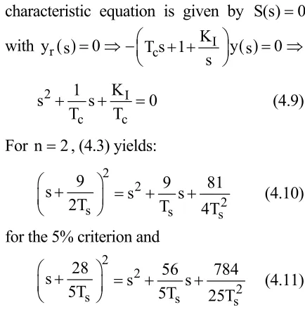
For n 2= , (4.3) yields: 2
2
2
s s s
9 9 81
s s s
2T T 4T
+
= + +
(4.10)
for the 5% criterion and 2
2
2
s s s
28 56 784
s s s
5T 5T 25T
+ = + +
(4.11)
for the 2% criterion. Comparing (4.9) with (4.10) and (4.11) in turn yields the required controller parameters for the chosen criterion:
5% s 5% 2% s 5%
c I c I
s s
T 9 5T 14
T ,K ,T ,K
9 4T 56 5T
= = = =
(4.12)
Note that the plant parameter, b, is not needed, indicating the extreme robustness of SMC.
r y (s) − 2 Plant b s u(s) y(s) c 1 T s+
+ S(s) max u + max u −
K
− KsI
+
Integral + SMC Controller − IPD Controller − 2 Plant b s
u(s) y(s)
p d
K +K s
+
I K
s r
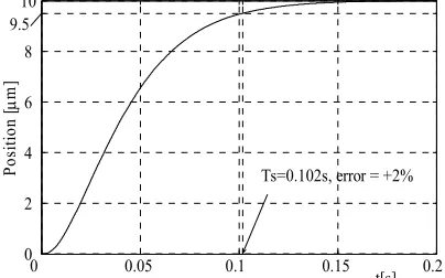
4.4 Experimental results
The plant hardware is briefly described at the beginning of section 4.1. For both controllers, the settling time is set to Ts =0.1s, a step reference position of 10 mµ is applied and the sampling frequency of the DSpace implementation is 40 kHz. For the SMC, the slope of the transfer characteristic realising
0 0.05 0.1 0.15 0.20
0 2 4 6 8 10
t[s]
Po
siti
on
, x
(
µ
m)
9.5
[image:9.595.320.529.237.381.2]Ts=0.102s, error = +2%
Fig. 4.3: Experimental IPD response (5% criterion).
0 0.05 0.08 0.1 0.15 0.2
0 5 10
t[s]
Po
siti
on
, x
[
µ
m]
[image:9.595.82.285.264.409.2]Ts=0.093s, error = -7% 0.98
Fig. 4.4: Experimental IPD response (2% criterion).
0 0.05 0.1 0.15 0.2 0
2 4 6 8 10
Po
si
tio
n [
µ
m]
Ts=0.102s, error = +2% 9.5
t[s]
Fig. 4.5: Experimental SMC response (5% criterion).
the boundary layer is K 2x10= 4. Figs 4.3 to 4.6 show the results. Comparison of the errors in the realised settling time with the theoretical ones in Table 3.1 shows some differences that are attributed to plant modelling errors but these are within acceptable limits for most applications.
0 0.05 0.1 0.15 0.2 0
2 4 6 8 10
Po
sitio
n [µ
m]
Ts=0.10, error = 0% 0.98
[image:9.595.83.285.424.553.2]t[s]
Fig. 4.6: Experimental SMC response (2% criterion).
5. Conclusions and Recommendations
Two settling time formulae have been derived for closed loop systems with coincident poles and their use in control systems design demonstrated. The experimental results show that the desired settling time is accurately realised. Extension to complex conjugate pole placement would be of interest as in a few cases a small amount of overshoot is desirable.
6. Acknowledgement
The author is very grateful to Paul Stadler of the Institute for Mechatronics at the Bern University of Science, Switzerland, for producing the DSpace based experimental results.
References
[image:9.595.83.285.593.719.2]P.A. Stadler, S.J. Dodds and H.G. Wild ‘Simultaneous High Precision Control of the Position and an Oscillatory Mode of a Vacuum Air Bearing Linear Drive’ Proceedings of the 5th International Symposium on Linear Drives
for Industry Applications, 116-119, 2005.