The Effects of Control Domain Size on Optimal Control Problem of Monodomain Model

The Effects of Control Domain Size on Optimal Control

Problem of Monodomain Model

Kin Wei Ng

Department of Mathematical Sciences

Faculty of Science

Universiti Teknologi Malaysia

81310 Johor Bahru, Malaysia

Ahmad Rohanin

Department of Mathematical Sciences

Faculty of Science

Universiti Teknologi Malaysia

81310 Johor Bahru, Malaysia

ABSTRACT

In this paper, we study the effects of the size of the control domain on the optimal control problem of monodomain model. The optimal control problem of monodomain model is a nonlinear optimization problem that is constrained by the monodomain model that represents the electrical behavior of the cardiac tissue. Two test cases with different sizes of control domain are considered, namely Test Case 1 and Test Case 2. Numerical results show that the excitation wavefront is successfully dampened out by the optimal applied current in both test cases. However, Test Case 2 (with smaller size of the control domain) requires more iteration as well as longer time to dampen the excitation wavefront. Our numerical results also indicate that higher current is required in the dampening process when the size of the control domain changed to a smaller one.

Keywords

Galerkin finite element method, Monodomain model, Optimal control, Cardiac electrophysiology

1.

INTRODUCTION

Optimal control problem of monodomain model was first proposed by Nagaiah et al. [1] and has been subsequently studied in [2, 3, 4, 5], with the control objective is to dampen the excitation wavefront of the transmembrane potential using optimal applied current. The optimal control problem of monodomain model is a nonlinear optimization problem that is constrained by the monodomain model that represents the electrical behavior of the cardiac tissue. The monodomain model is a well-known mathematical model extensively used in simulating cardiac electrical activity [6, 7]. It consists of a parabolic partial differential equation coupled to a system of nonlinear ordinary differential equations representing cell ionic activity.

Two types of optimization methods have been applied by researchers for solving the optimal control problem of monodomain model in the literature, which are nonlinear conjugate gradient method and Newton method. Nonlinear conjugate gradient method has low memory requirement but usually requires many iterations to converge to a solution. In contrast, Newton method is likely to converge with less iteration but requires higher memory storage.

The nonlinear conjugate gradient method is first employed by Nagaiah et al. [1] to solve the optimal control problem of monodomain model. Three variants of the nonlinear conjugate gradient method are chosen and compared, namely Polak-Ribière-Polyak (PRP) method [8, 9], Dai-Yuan (DY) method [10] and Hager-Zhang (HZ) method [11].

Later, Nagaiah et al. [2] proposed a second order optimization method, i.e. the Newton method, with the purpose to solve the optimal control problem of monodomain model efficiently. Numerical results indicate that the Newton method converges faster to the solution than the nonlinear conjugate gradient method. Furthermore, this second order optimization method is enhanced by Nagaiah and Kunisch [3] using adaptive grid refinement techniques.

Recently, Ng and Rohanin [5] applied the modified Dai-Yuan (MDY) method [12] for solving the optimal control problem of monodomain model. This modified version of the DY method is based on the idea of the modified BFGS method as proposed by Li and Fukushima [13]. Numerical results show that the MDY method performs quite well under Armijo line search, using only 38 iterations to converge to a solution. Note that the above studies focused on developing efficient numerical techniques to solve the optimal control problem of monodomain model. However, the effects of the size of the control domain on the optimal control problem of monodomain model still has not been studied. The purpose of this paper is therefore to study these effects using different sizes of the control domain in our numerical experiments.

2.

THE OPTIMAL CONTROL

PROBLEM OF MONODOMAIN MODEL

In this section, we present the optimal control problem governed by the monodomain model. Let 2 be the computational domain with Lipschitz boundary , _c be the control domain and _o be the observation domain. The optimal control problem of monodomain model is therefore given by









 

 





 

 

 

 

 

     

     

          

   

 

 





 



 

on , 0 ,

on , 0 ,

, 0 on , 0

, 0 in , 0

, 0 in , 0

s.t.

2 1 , min

0 0

0

2 2

w x w

V x V

T V

D

T f

t w

T I

I t V C V D

dt d I d

V I

V J

ion m

T

c e o

e

o c



 



(1)

where

e

i I I

D D

 



  



Here  is the regularization parameter, T is the final simulation time,  is the unit normal vector directed outwards from , D_i is the intracellular conductivity tensor,

 

xt

V , is the transmembrane potential,  is the surface-to-volume ratio of the cell membrane, C_m is the membrane capacitance per unit area, I_ion



V,w



is the current density flowing through the ionic channels, I_e

 

x,t is the extracellular current density stimulus, w

 

x,t are the ionic current variables, f



V,w



are the prescribed vector-value functions and  is the constant scalar used to relate the intracellular and extracellular conductivity tensors. Both functions Iion



V,w



and f



V,w



depend on the ionic model used. In this paper, a simplified two variable model, namely the Rogers-modified FitzHugh-Nagumo model [14] is chosen, which is given by





cwV

V V V V V c w V I p th

ion , 1 1 1  2

              





_       

 cw

V V c w V f p 4 3 ,

where V_p is the plateau potential, V_th is the threshold potential, and c1,c2,c3,c40 are positive parameters. Notice that the optimal control problem of monodomain model is a PDE-constrained optimization problem with I_e as the control variable while V and w as the state variables. The control variable I_e is chosen such that it is nontrivial only on _c and extended by zero on \_c.

3.

THE OPTIMIZE-THEN-DISCRETIZE

APPROACH

This section describes the numerical approach for solving the optimal control problem defined in (1). We adopt the optimize-then-discretize approach, where the infinite dimensional optimality system is derived first and the resulting optimality system is then discretized.

3.1

First Order Optimality System

For deriving the infinite dimensional optimality system, we defined Lagrange functional, L, as follows





dt d q f t w dt d p I I t V C V D dt d I d V T T ion m T c e o o c        _           _{ }              _{  } 

 

 

 



    2 1 0 0 0 2 2    L (2)

where p

 

x,t and q

 

x,t are Lagrange multipliers. The first order optimality system is stated by requiring stationarity of (2) with respect to the state



V,w



, adjoint

 

p,q and control

 

Ie variables, resulting in





 

 

0

:         

 I p f q

t p C p D

V_o m ion_{V V}

V  

L (3)

 

 

0

:  

  

 f q

t q p

I_{ionw w}

w 

L (4)





0

:        

 I I

t V C V

D _{m ion}

p  

L (5) 0 :     f t w q L (6) 0 1 1 :    p Ie I_e  _

L (7)

where

 

 _V denotes the partial derivative with respect to V ,

 

 w denotes the partial derivative with respect to w, and

o

V denotes the transmembrane potential in the observation domain. Next, the state and adjoint systems can be formed using (3) – (6) together with the following initial, terminal and boundary conditions.

 

x,0 V0, w

 

x,0 w0

V  

 

x,T 0, q

 

x,T 0 p



DV



0,



Dp



0 Consequently, the state system is given by









 

 

                        , 0 , and 0 , , 0 , , 0 0 w x w V x V V D f t w I I V D t V

Cm ion



 

(8)

while the adjoint system is given by





 

 

 

 





 

 

                           , 0 , and 0 , , 0 , , T x q T x p p D q f p I t q V q f p I p D t p C w w ion o V V ion m     (9)

Kunisch and Wagner [4] proved that the control-to-state mapping is well-defined for the optimal control problem in (1). This allows us to rewrite the cost functional in (1) as

 

I V

 

I d I d dt

J T c e o e e o c

 



            0 2 2 2 1

ˆ _{ (10)}

where (10) is known as the reduced cost functional. It follows that the reduced gradient is given by

 

I I p

J e e _



1 1

ˆ

As a result, the first order optimality system consists of the state system in (8), the adjoint system in (9) and the optimality condition in (7) that served as reduced gradient during computation.

3.2

Discretization of Optimality System

Galerkin finite element method in space and Crank-Nicolson method in time. For temporal discretization of the nonlinear ODEs in (8) and (9), the forward Euler method is used. Consequently, the discretized state system is given by

 

 

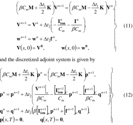
                                                , 0 , , 0 , , , , 2 2 2 1 2 1 1 1 1 0 0 ion w w V V f w w I I V V V K M V K M x x t C C t t C t C n n n m n m n n n n m n m    (11)

and the discretized adjoint system is given by

 

 

 

 





 

 

                                      _        _             , , , , , , , 2 2 1 1 1 1 2 1 1 1 1 1 1 2 1 1 1 1 0 q 0 p q f p I q q q f p I V p p p K M p K M ion ion T x T x t C C C t t C t C n w n n w n n n n m V n n m V n m o n n n n m n m      (12)

where M is the mass matrix,K is the stiffness matrix, t1

and t₂ are the local time-steps.

4.

OPTIMIZATION PROCEDURE

In this paper, the optimization stage is carried out using the modified conjugate gradient method, that is, the MDY method. In order to compute the step-length, the standard Armijo line search is used. Given an initial step-length 0 , 

 

0,1 and 

 

0,1 , choose kmax



,,2,



such that



k k k

  

k k

 

kT k

J J

JˆIe d  ˆIe ˆIe d (13) For the stopping criteria, we consider the following

   

1 3

10 ˆ

ˆ k _ k _ 

J

JIe Ie and

 



 



k k

J JˆIe 10 1 ˆIe

3 _ 

 

(14)

The algorithm for solving the discretized optimal control problem is given as follows

Optimization Algorithm:

Step 0. Provide an initial guess I0e and set k0. Step 1. Solve the discretized state system in (11).

Step 2. Evaluate the reduced cost functional Jˆ

 

Ike . Step 3. Use the result obtained in Step 1 to solve the

discretized adjoint system in (12).

Step 4. Update the reduced gradient J

 

Ike Ike _pk 1

1

ˆ _.

Step 5. For k1, check the stopping criteria in (14). If one of them is met, then stop.

Step 6. Compute the direction

 

 

1

ˆ _{, 0,}

ˆ _{, 0,}

k

k

k k k

J if k

J   if k

         e e I d I d where

 

     

1



1 1 1



2 ˆ ˆ ˆ     _{  }   k k k k k T k k k J J J d I I d I e e e   

 



    





                       2 1 1 1 1 1 2

3 ˆ ˆ

, 0 max ˆ 10 k k k k T k k k

k J J

J

d

I I d

I e e

e

  

Step 7. Compute step-length _k _{that satisfies condition in} (13).

Step 8. Update the control variable I_ek1I_ekkdk. Set 1

 k

k and go to Step 1.

5.

NUMERICAL EXPERIMENTS

5.1

Experiment Setup

A two dimensional computational domain 

   

0,10,1 of size 11 cm2 is considered in our numerical experiments and the final simulation time is set to be T2ms. The computational domain  is discretized into 8192 triangular elements and the temporal discretization were set to

2 1 2.5 10

t 

   ms and t2 103



[image:3.595.56.282.121.333.2]

  ms. Table 1 lists the parameters that we used in our numerical experiments, with some of them adopted from [16].

Table 1. Parameters used in numerical experiments

Parameter Value Units

 3

10 cm1

m

C 3

10 mF 2

cm

l i

D 3

10

3  Scm1

t i D 4 10 1525 .

3   Scm1

th

V 1

10 3 .

1  mV

p

V 2

10 mV

1

c 1.5 mScm2

2

c 4.4 mS 2

cm 3 c 2 10 2 .

1   ms1

4

c 1 dimensionless

 4

10 dimensionless

 1

10 062 .

7   dimensionless

 1 dimensionless

 4

10 dimensionless

 1

10 dimensionless

Figures 1 and 2 illustrate the positions of the sub-domains in the computational domain  for Test Case 1 and Test Case 2, respectively. From the figures, _c1 and _c2 are the control domains, ~_c1 and ~_c2 are the neighborhoods of the control domains,



1 2



~ ~

\ c c

o  

[image:4.595.319.539.130.310.2]

domain and _exi_o is the excitation domain. In our experiment, the control domain might correspond to implantable cardioverter defibrillator (ICD) implanted in the chest of a patient to avoid sudden cardiac death. Consequently, the control domain for Test Case 1 can be interpreted as a heavier (with bigger size) ICD while the control domain for Test Case 2 can be interpreted as a lightly (with smaller size) ICD that can be placed into the chest.

[image:4.595.56.278.168.347.2]

Fig 1: Computational domain  and its sub-domains for Test Case 1

Fig 2: Computational domain  and its sub-domains for Test Case 2

The initial values for the state variables are given as

 

 

 



otherwise,

mV, 0

, mV, 105 0

, x exi

x

V and w

 

x,0 0, x

On the other hand, the initial value for the control variable is set to be zero in the control domain, i.e. no current is applied at the beginning of the numerical experiments.

5.2

Experiment Results

In this section, we present the experiment results for Test Case 1 and Test Case 2. The minimum values of the reduced cost functional Jˆ

 

Iek along the optimization process for both test cases are depicted in Figure 3. As shown in the figure,

Test Case 1 requires 18 iterations to converge to the solution while Test Case 2 takes 30 iterations. This result implies that when the size of the control domain is reduced to a smaller one, more iteration is required to dampen the excitation wavefront of the transmembrane potential.

Fig 3: Minimum values of Jˆ for 2 ms of simulation time

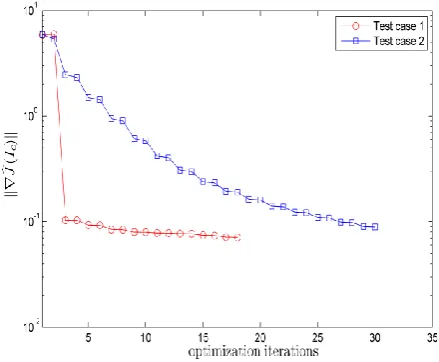
Figure 4 depicts the corresponding norm of reduced gradient

 

k

JˆIe

 for Test Cases 1 and 2. As shown in Figure 4, the gradient for Test Case 1 is decreased sharply at the beginning of optimization process, followed by a smooth decrease to the end. On the other hand, the gradient for Test Case 2 is decreased smoothly started from the beginning to the end of iterations. This phenomenon happens because the applied current is unable to give a significant effect to the dampening process if a small size control domain is used.

Fig 4: Norm of reduced gradient of Jˆ for 2 ms of

simulation time

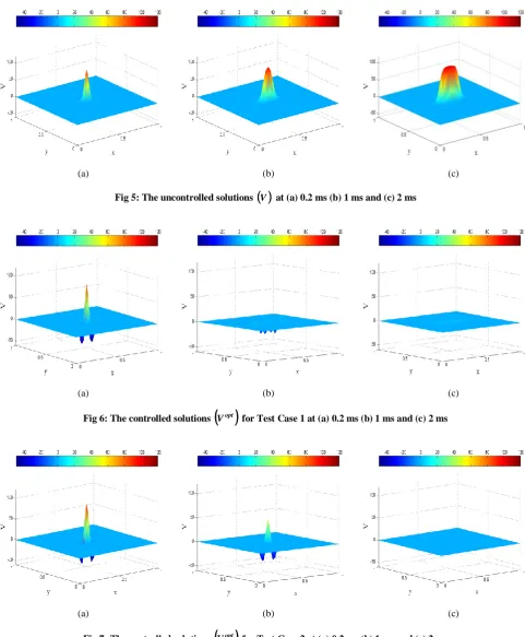
[image:4.595.57.276.393.576.2] [image:4.595.316.536.456.637.2]

wavefront of the transmembrane potential will continue to propagate to the computational domain if the control is not switched on. For the optimally controlled case, the excitation wavefront is successfully dampened out by the optimal applied current Iopt_e for both test cases. Observe that, the

excitation wavefront for Test Case 1 is almost completely dampened out at time 1 ms, however, this is not the case for Test Case 2. For Test Case 2, longer time is needed to dampen out the excitation wavefront if compared to Test Case 1.

[image:5.595.54.536.142.725.2]

(a) (b) (c)

Fig 5: The uncontrolled solutions

 

V at (a) 0.2 ms (b) 1 ms and (c) 2 ms

(a) (b) (c)

Fig 6: The controlled solutions

 

Vopt for Test Case 1 at (a) 0.2 ms (b) 1 ms and (c) 2 ms

(a) (b) (c)

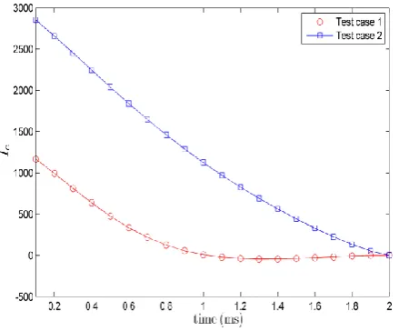
Lastly, Figure 8 displays the optimal applied current opt

e I over the time evolution, at a fixed point in the control domain, i.e.





c

[image:6.595.56.276.140.322.2]

x 0.5625,0.5 . As shown in the figure, Test Case 2 requires higher current than Test Case 1 in the effort to dampen out the excitation wavefront.

Fig 8: Time evolution of the optimal applied current

 

I_eopt

at point x



0.5625,0.5



6.

CONCLUSIONS

In this paper, we have presented the numerical experiment results for the optimal control problem of monodomain model for two test cases. Test Case 1 consists of a bigger size of the control domain, while Test Case 2 consists of a smaller one. Our results show that when the size of the control domain has changed to a smaller one, more iteration is required to dampen the excitation wavefront. Besides that, longer time is also needed for dampening the excitation wavefront if a small size control domain is used. Moreover, by implanting a more lightly ICD, higher electrical shock is required to be delivered to the patient in order to restore the normal heart rhythm. Alternatively, if a heavier ICD is implanted in a patient, lower electrical shock will be delivered to the patient for restoring normal heart rhythm. If we can balance the trade-off between the size (weight of ICD) and the current (electrical shock delivered by ICD), it will be good news for patients that decide to implant ICD.

7.

ACKNOWLEDGMENTS

The work is financed by Zamalah Scholarship provided by Universiti Teknologi Malaysia and the Ministry of Higher Education of Malaysia.

8.

REFERENCES

[1] Nagaiah, C., Kunisch, K., and Plank, G. 2011. Numerical solution for optimal control of the reaction-diffusion equations in cardiac electrophysiology. Comput. Optim. Appl. 49, 149-178.

[2] Nagaiah, C., Kunisch, K., and Plank, G. 2009. Second order numerical solution for optimal control of

monodomain model in cardiac electrophysiology. In Proceedings of ALGORITMY.

[3] Nagaiah, C. and Kunisch, K. 2011. Higher order optimization and adaptive numerical solution for optimal control of monodomain equations in cardiac electrophysiology. Appl. Numer. Math. 61, 53-65. [4] Kunisch, K. and Wagner, M. 2011. Optimal control of

the bidomain system (I): The monodomain approximation with the Rogers-McCulloch model. Nonlinear Anal.: Real World Appl. 13 (4), 1525-1550. [5] Ng, K. W. and Rohanin, A. 2012. Numerical solution for

PDE-constrained optimization problem in cardiac electrophysiology. Int. J. Comput. Appl. 44 (12), 11-15. [6] Belhamadia, Y., Fortin, A., and Bourgault, Y. 2009.

Towards accurate numerical method for monodomain models using a realistic heart geometry. Math. Biosci. 220 (2), 89-101.

[7] Shuaiby, S. M., Hassan, M. A., and El-Melegy, M. 2012. Modeling and simulation of the action potential in human cardiac tissues using finite element method. J. Commun. Comput. Eng. 2 (3), 21-27.

[8] Polak, E. and Ribière, G. 1969. Note sur la convergence de méthodes de directions conjuguées. Rev. Francaise Informat. Recherche Opérationnelle. 16, 35-43. [9] Polyak, B. T. 1969. The conjugate gradient method in

extreme problems. USSR Comp. Math. Math. Phys. 9, 94-112.

[10] Dai, Y. H. and Yuan, Y. 1999. A nonlinear conjugate gradient method with a strong global convergence property. SIAM J. Optim. 10 (1), 177-182.

[11] Hager, W. W. and Zhang, H. 2005. A new conjugate gradient method with guaranteed descent and an efficient line search. SIAM J. Optim. 16, 170-192.

[12] Zhang, L. 2009. Two modified Dai-Yuan nonlinear conjugate gradient methods. Numer. Algor. 50, 1-16. [13] Li, D. H. and Fukushima, M. 2001. A modified BFGS

method and its global convergence in nonconvex minimization. J. Comput. Appl. Math. 129, 15-35. [14] Rogers, J. M. and McCulloch, A. D. 1994. A

collocation-Galerkin finite element model of cardiac action potential propagation. IEEE Trans. Biomed. Eng. 41, 743-757. [15] Qu, Z. and Garfinkel, A. 1999. An advanced algorithm

for solving partial differential equation in cardiac conduction. IEEE Trans. Biomed. Eng. 46 (9), 1166-1168.