http://dx.doi.org/10.4236/jtts.2014.43023
Real-Time Road Traffic Anomaly Detection
Jamal Raiyn
1, Tomer Toledo
21Faculty of Exact Science, Computer Science Department, Al Qasemi Acedemic College, Baqa Al Qarbiah, Israel 2Faculty of Civil and Environmental Engineering, Department of Transportation Engineering, Technion, Haifa,
Israel
Email: [email protected], [email protected]
Received 14 February 2014; revised 12 March 2014; accepted 7 April 2014
Copyright © 2014 by authors and Scientific Research Publishing Inc.
This work is licensed under the Creative Commons Attribution International License (CC BY).
http://creativecommons.org/licenses/by/4.0/
Abstract
Many modeling approaches have been proposed to help forecast and detect incidents. Accident has received the most attention from researchers due to its impacts economically. The traffic gestion costs billions of dollars to economy. The main reasons of major percentage of traffic con-gestion are the incidents. Road accidents continue to increase in digital age. There are many rea-sons for road accidents. This paper will discuss and introduce new algorithm for road accident detection. Various forecast schemes have been proposed to manage the traffic data. In this paper we will introduce road accident detection scheme based on improved exponential moving average. The proposed traffic incident detection algorithm is based on the automatic exponential moving average scheme. The detection algorithm is based on analyzing the collected traffic flow parame-ters. The detection algorithm is based on analyzing the collected traffic flow parameparame-ters. In addi-tion a real-time accident forecast model was developed based on short-term variaaddi-tion of traffic flow characteristics.
Keywords
Anomaly Traffic, Detection Scheme, Moving Average, Intelligent Transportation System
1. Introduction
travelers. The third strategy is to focus on efficient and intelligent utilization of the existing transportation infra-structures. This strategy is a best trade-off and gains more and more attention. Currently, the Intelligent Trans-portation System (ITS) is the most promising approach to implementation of the third strategy. Various forecast schemes [6]-[9] have been proposed to manage the travel flow information. Meanwhile the robustness and ac-curacy of the exponential smoothing forecast are high and impressive. This paper reports on the performance of three moving average techniques in predicting average travel speeds up to 10 minutes ahead of time. The ad-vantage of the exponential smoothing algorithm is simple. However its forecast precision is not high. If a high forecast precision is requested, it is necessary to consider the real-time information includes the non-conditions events. This paper introduces road accident detection scheme. Road accident detection scheme is focused on real-time information. The real-time information has been achieved to update the historical adaptive informa-tion.
To optimize the detection algorithm we have collected travel data by the mobile phone. For a successful fore-cast of traffic flow, it ought to apperceive the variety of environment and can adjust the parameters automatical-ly. Furthermore it is important that the forecast model takes into consideration the abnormal conditions that oc-cur in real-time [4] [10] [11].
The paper is organized as fellow: Section 2 describes the methodology of road accidents detection scheme. Section 3 and section 4 discuss the performance analysis of the proposed detection scheme and illustrate the si-mulation results.
2. Methodology
This section presents a methodology to detect road accidents based on travel time variations. We consider acci-dent during peak periods (i.e., morning or afternoon) and during non-peak periods. The observed traffic data consists of normal and abnormal (accident) travel data. The abnormal record is at least 30 km/h lower traffic speed than the average speed of all records at the same time on the same day of the week. The threshold of 30km/h is a symbolic value of the smallest speed change that people would consider “abnormal”. Threshold de-termination depends on the travel observation data. Equation (1) will be used to forecast the accident scheme.
(
1, ,)
(
, ,) (
1)
(
, ,)
tt t+ k acci = ×α tt t k acci + −α ×EMA t k acci (1)
Alpha can be expressed as follows:
( )
( )
11 Var k
E k
α =
+
where Var(k) is the variance of the expected number of crashes at the reference sites. E(k) is the expected num-ber of crashes at these reference sites.
2.1. Section Mutual Influence
In the real-time forecasting we take into consideration the effect of the upstream (UP) and downstream (DS) as illustrates in Equation (2).
(
1,)
(
1,)
1 desired 2 UP 3 DSH
tt t+ k =tt t+ k + ×
γ
+ ×γ
+ ×γ
(2)where
( )
( )
desired=ttM t k, −ttH t k,
(
)
(
)
upstearm=ttM t k, − −1 ttH t k, −1
(
)
(
)
downstream=ttM t k, + −1 ttH t k, +1
( )
(
)
(
)
abnormal , 1, 1,
( ) (
)
(
tt t k, tt t 1,k)
δ = ∆ − +
k is the desired section, (k − 1) is the upstream section, (k + 1) is the downstream section.
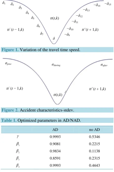
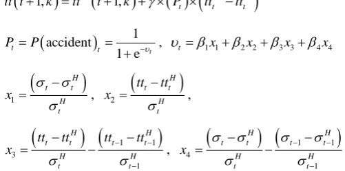
Figure 1 and Figure 2 illustrate the abnormal condition in the up and down stream.
2.2. Accident Detection Strategy
The performance of an incident detection system is determined on two levels: data collection and data pro- cessing. Data collection refers to the detection/sense/surveillance technologies that are used to obtain traffic flow data. Data processing refers to the algorithms used for detecting and classifying incidents through analyzing the traffic parameters from detectors or sensors for the purpose of alerting observers of the occurrence, severity, and location of an incident. The hybrid of data collection strategies and data processing methodologies results in a variety of solutions for incident detection. The main task of the proposed accident detection (AD) algorithm is to identify and distinguish different traffic modes in Table 1. It depends on an upstream occupation increase and a downstream occupation decrease at the level of loop detector where an incident happened. This algorithm com-pares a value of a traffic flow parameter with a known value. The algorithm trusts that an upstream occupation will increase and downstream occupation will decrease where an incident happened. In traffic incident detection, a time sequence is used to describe a traffic state. When a current measured value is deviated from the output of the algorithm seriously, the algorithm will think that an incident has occurred. The time sequence analytic algo-rithms include a moving average algorithm, an exponential smoothing algorithm.
• The accident characterized by temporal variation of speed at fixed road section (location) expressed as the coefficient of variation in speed.
• The spatial variation of speed along road sections expressed as the difference in speed between upstream and downstream location (Q).
tt(t,k)
tt−(t − 1,k) tt+(t + 1,k)
−δ15
−δ14
−δ13
−δ12
−δ11
−δ10
−δ9 δ7
δ6 δ5 δ4 δ3 δ2 δ1
δ
Figure 1.Variation of the travel time speed.
tt−(t − 1,k) tt+(t + 1,k)
σpree σduring σafter
tt(t,k)
[image:3.595.197.428.380.727.2]Figure 2. Accident characteristics-stdev.
Table 1. Optimized parameters in AD/NAD.
AD no AD
γ 0.9993 0.5346
1
β 0.9081 0.2215
2
β 0.9834 0.1138
3
β 0.8591 0.2315
4
( )
, 1(
, 2)
Q= tt t s −tt t s (3)
where tt t s
( )
, 1 , tt t s(
, 2)
average speeds computed over period of t upstream and downstream of a road sec-tions, respectively (km/h).2.3. Incident-Influence Traffic Data
An incident occurring on section i within time interval t is considered to have a significant impact on traffic when traffic measurements from the upstream and downstream stations satisfy the following conditions:
1) The difference between upstream speed si, t and downstream speed si + 1, t is greater than the threshold value;
2) The ratio of the difference between the upstream and downstream speeds to the upstream speed (si, t – si + 1, t/si, t,is greater than the threshold value;
3) The ratio of the difference between the upstream and downstream speeds to the downstream speed (si, t − si + 1, t)/si + 1, t is greater than the threshold value.
The abnormal record shows that at least 30 km/h lower traffic speed than the average speed of all records at the same time on the same day of the week. The threshold of 30 km/h is a symbolic value of the smallest speed change that people would consider “abnormal”. The vehicle speed starts to decrease in upstream however the speed in downstream starts to increase.
When an incident occurs between stations k and k + 1, the congestion causes a clear difference between the occupancies of the upstream and the downstream stations as illustrates Figure 3.
( ) (
)
( )
, 1,
threshold ,
tt k t tt k t
tt k t
− +
> (4)
( )
(
)
(
)
, ) 1,
threshold 1,
tt k t tt k t
tt k t
− +
>
+ (5)
(
)
(
)
1
1 Mean accidents
n i i
N = µ σ
=
∑
− (6)standard deviation,Nnumber of the acidents.
σ
2.4. Real-Time Accident Detection
The travel time forecast model considers the incident and non-incident conditions. We make different between: • Accident during peak time (morning/afternoon);
• Accident during regular time; • Heavy accident;
• Light accident.
The accident is cleared at current time t in section s, the duration is known and the speed is considered to be 30 km reduced of the average speed.
μ − σ1
σpree σafter
σduring
μ + σ1
tt(t,k)
B
A C
(
1,)
H(
1,)
( )
(
M H)
t t t
tt t+ k =tt t+ k + ×γ P × tt −tt
(
)
1accident
1 e t
t t
P =P = −υ
+ , υt =β1 1x +β2x2+β3 3x +β4x4
(
)
1 H t t H tx σ σ
σ
−
= , 2
(
)
H t t H t tt tt x σ − = ,
(
) (
1 1)
3
1
H H
t t t t
H H
t t
tt tt tt tt
x
σ σ
− −
−
− −
= − , 4
(
) (
1 1)
1
H H
t t t t
H H
t t
x σ σ σ σ
σ σ
− −
−
− −
= −
where X denotes the vector of predictor variables. β is the vector of coefficient associated with the predictor va-riables. and can be computed according to the binary logit model. νt is the logit link function (which is a linear
combination of the predictor variables).
2.5. Accident Probability
Based on statistical measurements of historical information and real information, the forecast model can esti-mate the occurrence of abnormal conditions without external information as express Equation (7) and Equation (8).
(
1,)
(
1,)
(
( )
,( )
,)
F H M H
acc acc acc acc
tt t+ k =EMA t+ k +δ tt t k −tt t k (7)
(
)
(
)
(
( )
( )
)
Corrections needed epsilon
1, 1, , ,
F H M H
acc acc acc
tt t k EMA t k δ tt t k tt t k
=
+ = + + −
(8)
where,
( )
(
)
(
( )
)
(
mean EMAnormal k t, mean EMAabnormal k t,)
ε = −
( )
(
)
{
(
( )
)
(
)
}
hist
accident , i , th hist
P tt t k =P σ tt t k >δ (9)
(
)
(
)
{
(
( )
)
(
( )
)
}
real hist
accident 1, i , max ,
M
i i
P tt t+ k =P σ tt t k > σ tt t k (10)
where:
( )
(
)
2 1 hist
th M th
δ >δ
( )
(
ttM t k,)
(
ttM(
t 1,k)
)
σ >σ −
( )
,( )
,M H
tt t k >tt t k
( )
,(
1,)
M H
tt t k >tt t− k
The Total number of the expected accident is expressed as following:
(
) (
real)
accident 1 accident
M
E N = −P ×n (9)
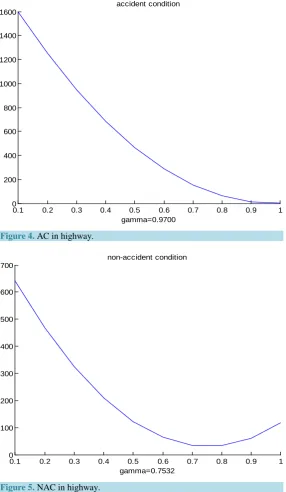
2.6. Smoothed Parameter Optimization
[image:5.595.186.437.93.217.2]To increase the exponential moving average forecast accuracy in real-time, the smoothed parameter alpha and gamma in Equation (4) should be optimized. Figure 4 illustrated the value of the optimized smoothed parameter gamma in real-time accident conditions.
Figure 4. AC in highway.
Figure 5.NAC in highway.
3. Performance Analysis
There are various measures of forecasting accuracy techniques proposed in the literature [5] [12]-[15]. The aim of this study is to evaluate forecast accuracy travel observations. The forecasting accuracy techniques are used to be able to select the most accurate forecast scheme. The forecasting performance of the various models and the measures of the predictive effectiveness was evaluated using various summary statistics. The comparing expe-riments are carried out under normal traffic condition and abnormal traffic condition to evaluate the performance of four main branches of forecasting models on direct travel time data obtained by license plate matching (LPM). The MAE is a measure of overall accuracy that gives an indication of the degree of spread, where all errors are assigned equal weights. The MSE is also a measure of overall accuracy that gives an indication of the degree of spread, but here large errors are given additional weight. It is the most common measure of forecasting accuracy.
0.1 0.2 0.3 0.4 0.5 0.6 0.7 0.8 0.9 1
0 200 400 600 800 1000 1200 1400 1600
gamma=0.9700 accident condition
0.1 0.2 0.3 0.4 0.5 0.6 0.7 0.8 0.9 1
0 100 200 300 400 500 600 700
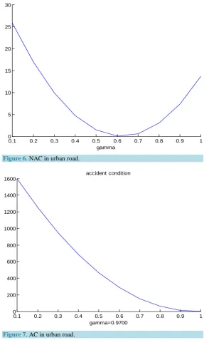
Figure 6.NAC in urban road.
Figure 7. AC in urban road.
Often the square root of the MSE, RMSE, is considered, since the seriousness of the forecast error is then de-noted in the same dimensions as the actual and forecast values themselves. Mean square percentage error (MSPE) is the relative measure that corresponds to the MSE. The more commonly used measure is the root mean square percentage error (RMSPE). Theil’s Coefficient is another statistical measure of forecast accuracy. One specification of Theil’s compares the accuracy of a forecast model to that of a naive model. A Theil’s greater than 1.0 indicates that the forecast model is worse than the naïve model; a value less than 1.0 indicates that it is better. The closer U is to 0, the better the model.
4. Simulation Results
The travel observation data consists of normal and abnormal (accident) travel data. Figure 8(a)and Figure 8(b)
illustrate the abnormal conditions in up and download stream in peak hours. However Figure 8(c)illustrates the abnormal condition in no peak hours.
0.1 0.2 0.3 0.4 0.5 0.6 0.7 0.8 0.9 1
0 5 10 15 20 25 30
gamma
0.1 0.2 0.3 0.4 0.5 0.6 0.7 0.8 0.9 1
0 200 400 600 800 1000 1200 1400 1600
(a)
(b)
[image:8.595.113.512.79.706.2](c)
Figure 8.(a) Travel time variation in AC; (b) Travel time variation in AC; (c) Travel time variation in AC.
967 968 969 970 971 972 973 974
15 20 25 30 35 40
Observation [2.5min]
S
peed [
k
m
/hr
]
start point
end point
10 15 20 25
20 25 30 35 40 45
obserations[monday-07-09-2009/19:23-20:01]
s
peed[
k
m
/hr
]
2 4 6 8 10 12 14
25 30 35 40 45 50 55 60 65 70
observations[saturday-24-10-2009-20:58-21:26]
s
peed[
k
m
/hr
Table 2 and Table 3illustrate the performance analysis of exponential moving average scheme based on his-torical and real time forecasting. The comparison has been introduced based on accident and non accident con-ditions.
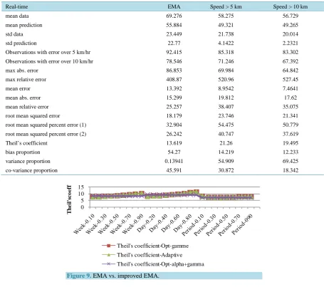
[image:9.595.88.540.189.716.2]Table 4describes the comparison of exponential moving average scheme based on sorted data that the dif-ference between two neighbor observations is bigger than 5 km and 10 km.Figure 9 illustrates the comparison between exponential moving average and improved exponential moving average.
Table 2. Hist vs. real-time in NAC.
Non-Accident Condition Hist Real
mean data 67.805 67.805
mean prediction 65.622 66.798
std data 17.809 17.809
std prediction 18.682 16.968
Observations with error over 5 km/hr 33.086 31.293
Observations with error over 10 km/hr 17.385 15.735
max abs. error 73.39 73.264
max relative error 587.12 586.11
mean error 2.183 1.0076
mean abs. error 6.6768 5.472
mean relative error 12.238 10.562
root mean squared error 12.452 9.2418
root mean squared percent error (1) 26.42 23.514
root mean squared percent error (2) 18.364 13.63
Theil’s coefficient 9.0011 6.6476
bias proportion 3.0737 1.1886
variance proportion 0.49122 0.82716
[image:9.595.84.539.461.719.2]co-variance proportion 96.435 97.984
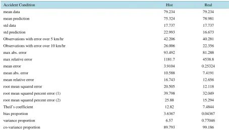
Table 3. Hist vs. real-time in AC.
Accident Condition Hist Real
mean data 79.234 79.234
mean prediction 75.324 78.981
std data 17.737 17.737
std prediction 22.993 16.673
Observations with error over 5 km/hr 42.206 40.281
Observations with error over 10 km/hr 26.006 22.356
max abs. error 93.492 81.288
max relative error 1181.7 4538.8
mean error 3.9104 0.25324
mean abs. error 10.588 7.4191
mean relative error 16.743 12.656
root mean squared error 20.505 12.118
root mean squared percent error (1) 39.798 32.049
root mean squared percent error (2) 25.88 15.294
Theil’s coefficient 12.82 7.4844
bias proportion 3.6367 0.04367
variance proportion 6.57 0.77046
Table 4. Up- and downstream effect.
Real-time EMA Speed > 5 km Speed > 10 km
mean data 69.276 58.275 56.729
mean prediction 55.884 49.321 49.265
std data 23.449 21.738 20.014
std prediction 22.77 4.1422 2.2321
Observations with error over 5 km/hr 92.415 85.318 83.302
Observations with error over 10 km/hr 78.546 71.246 67.392
max abs. error 86.853 69.984 64.842
max relative error 408.87 520.96 527.45
mean error 13.392 8.9542 7.4641
mean abs. error 15.299 19.812 17.62
mean relative error 25.257 38.407 35.075
root mean squared error 18.179 23.746 21.341
root mean squared percent error (1) 32.904 54.475 50.779
root mean squared percent error (2) 26.242 40.747 37.619
Theil’s coefficient 13.619 21.26 19.495
bias proportion 54.27 14.219 12.233
variance proportion 0.13941 54.909 69.425
[image:10.595.83.539.99.502.2]co-variance proportion 45.591 30.872 18.342
Figure 9. EMA vs. improved EMA.
4. Conclusion
Analysis of the road incidents based on the speed variation is not robust enough to develop real-time forecast model. Because a speed observation can be zero when there is no vehicle, or the system collects a wrong speed observation, in this case, the computation of CVS can be done in many variations.
References
[1] Ronen, B., Coman, A. and Schragenheim, E. (2001) Peak Management. International Journal of Production Research, 39, 3183-3193. http://dx.doi.org/10.1080/00207540110054588
[2] Tu, H., Van Lint, H. and Van Zuylen, H. (2008) The Effects of Traffic Accidents on Travel Time Reliability. IEEE Conference on Intelligent Transportation Systems, Beijing, 12-15 October 2008.
[3] Wang, Z. and Murray-Tuite, P. (2010) Modeling Incident-Related Traffic and Estimating Travel Time with a Cellular Automaton Model. Proceedings of Transportation Research Board’s 89th Annual Meeting CD-ROM, 10-14 January 2010, Washington, DC.
[4] Wild, D. (1997) Short-Term Forecasting Based on a Transformation and Classification of Traffic Volume Time Series. International Journal of Forecasting, 13, 63-72. http://dx.doi.org/10.1016/S0169-2070(96)00701-7
[5] Zheng, X. and Liu, M. (2009) An Overview of Accident Forecasting Methodologies. Journal of Loss Prevention in the Process Industries, 22, 484-491. http://dx.doi.org/10.1016/j.jlp.2009.03.005
0 5 10 15
T
h
e
il's
c
o
e
ff
Theil's coefficient-Opt-gamme
Theil's coefficient-Adaptive
[6] Andrada-Felix, J. and Fernandez-Rodriguez, F. (2008) Improving Moving Average Trading Rules with Boosting and Statistical Learning Methods. Journal of Forecasting, 27, 433-449. http://dx.doi.org/10.1002/for.1068
[7] Guin, A. (2006) Travel Time Prediction Using a Seasonal Autoregressive Integrated Moving Average Time Series Mode. Proceedings of the IEEE Intelligent Transportation Systems Conference, Toronto, 17-20 September 2006, 493- 498.
[8] Lv, Y. and Tang, S. (2010) Real-time Highway Traffic Accident Prediction Based on the K-Nearest Neighbor Method. International Conference on Measuring Technology and Mechatronics Automation, Volume 3, 547-550.
[9] Xia, J (2010) Predicting Freeway Travel Time under Incident Condition. Proceedings of Transportation Research Board’s 89th Annual Meeting CD-ROM, 10-14 January 2010, Washington, DC.
[10] Alger, M. (2004) Real-Time Traffic Monitoring Using Mobile Phone Data. Proceedings of 49th European Study Eu-ropean Study Group with Industry, Oxford, United Kingdom.
[11] Stephanedes, Y.J., Michalopoulos, P.G. and Plum, R.A. (1981) Improved Estimation of Traffic Flow for Real-Time Control. Transportation Research Record, 795, 28-39.
[12] Jo, H., Lee, B., Na, Y.-C., Lee, H. and Oh, B. (2007) Prioritized Traffic Information Delivery Based on Historical Data Analysis. Proceedings of the 2007 IEEE Intelligence Transportation Systems Conference, Seattle, September 30-Oc- tober 3 2007, 568-573.
[13] Karim, A. and Adeli, H. (2003) Fast Automatic Incident Detection on Urban and Rural Freeways Using Wavelet Energy Algorithm. Journal of Transportation Engineering, 129, 57-68.
http://dx.doi.org/10.1061/(ASCE)0733-947X(2003)129:1(57)
[14] Lee, H., Chowdhury, K.N. and Chang J. (2008) A New Travel Time Prediction Method for Intelligent Transportation Systems. Springer-Verlag, Berlin, 473-483.
currently publishing more than 200 open access, online, peer-reviewed journals covering a wide range of academic disciplines. SCIRP serves the worldwide academic communities and contributes to the progress and application of science with its publication.
Other selected journals from SCIRP are listed as below. Submit your manuscript to us via either