Numerical Analysis in Econom(etr)ic
Softwares: the Data-Memory Shortage
Management
Buda, Rodolphe
Modem - University of Paris 10
2005
Online at
https://mpra.ub.uni-muenchen.de/9145/
Softwares: the Data-Memory Shortage
Management
Rodolphe Buda
Economix
∗-
UMR 7166 CNRS
University of Paris 10
2005 (Revised 2007)
Summary
The econometricians and the economic modelers have to know and use numerical analysis not only to have a good understand-ing of their results, but sometimes to built their own tools. The increasing tendency to the use of large-scale models leads the softwares to reach the limit of the saturation of the Data-Memory. In this paper, we present an intuitive procedureDMT - i.e. Disk-Matrix Technique - which could help econom(etr)ic software de-velopers to correct the problem of the data-memory shortage dur-ing the builddur-ing of their own software.
Key-words : Algorithms ; Numerical Analysis ; Econom(etr)ic
Softwares ; Operating System ; Data-Memory ; Data Storage
JEL Classification: C15, C82, C87
⋆- Please read "economic and/or econometric".
∗[email protected] - [email protected]-T01-40-97-77-89 -v 01-47-21-46-89 -B200, Avenue de la République, Bât.G 610-C, 92001 NANTERRE Cedex - FRANCE
Econometricians and Economic Modelers usually use black boxes during theirs works1. Most of them use the metalanguage of softwares such as GAMS, MATLAB, MAPLE, Mathematica, SAS, GAUSS, G, and so on. However, econo-metricians and/or economic modelers have to take part to the building of the econom(etr)ic softwares2. That is a condition of understanding between develop-ers and usdevelop-ers - see [1, 3, 4, 10]. Thus, some other prefer to use primary languages such as C, Fortran, Java, Pascal and so on to implement their own procedures [11, 9]. Our paper reports some algorithmic problems we had to solve in building a multi-dimensional3economic modelling software (SIMUL i.e. SystèmeIntégré deModélisation mULtidimensionnelle)4. Since the 70th, the econometric mod-elers developed large-scale models [19] and this use should never decrease in the future, especially if we consider the micro-simulation modelling, the agent-based computational economics, or the artificial societies simulations. That means the software often reach the limits of the Data-memory. Some languages don’t man-age data-memory efficiently5. Even if the memory of computers increases, the size of the data-memory of such language is limited to 640 Ko - e.g. : Turbo-Pascal6. An algorithm has already developed [12] which uses hard disk and a buffer to solve this trouble. However, in this paper we present another algorithm only using hard disk to storage the too large arrays - technique called "disk-matrix technique" (DMT). Such algorithms increase the size of array in programs with-out decreasing readability of the program, but the disk-access delay is longer than the RAM-access delay.
In the first part, we’ll present the solution of the two dimensional problem, then we’ll generalize it in presenting the solution of the multi-dimensional problem. In the second part, we’ll expose the implementation of our algorithm to the matrix
1
- Not at the begin of the econometric period, during the econometricians have to built their programs. About this period, see [15]
2
- Despite of this fact, "There is no ideal software" [20]. 3
- Multi-regional (r), multi-sectoral (s), multi-periodical (t) analysis. 4
- The building of this software is integrated in the economic thesis we are finishing, "Mod-élisation multi-dimensionnelle et analyse multirégionale de l’économie française" under the su-pervision of the Professor Raymond Courbis. Our algorithm has been integrated in the Data bank management moduleGEBANK. This software usually can quickly estimate multi-dimensional econometric equations and solve the whole system: we only need an instruction to implement such equations :Yr,s
t =X
r,s
t .a r,s+ε
r,s
t . So it’s divided into some modules (estimation, data bank
management, resolving, etc.). For an overview ofSIMUL software, see our papers [6, 7]. 5
- As computational economics’ referees said us, Windows 95 introduced virtual memory in Microsoft’s line of operating systems and it has been used in every subsequent version of Windows. It automatically uses disk space if RAM proves insufficient for a program. Further, the limits are quite large today. Windows XP, currently the most common version, supports 4GB of RAM with up to 2 GB per per process. We agree with this, however, we consider this technique useful in the perspective of a very large simulation.
6
product. The third part will present the application of the DMT to the matrix inversion procedure. Then we’ll discuss the relevance of this technique.
1. The Two Dimensional Problem
The location of an element in a matrix is given by the rowiand column jranks. In a vector, there is nor row neither column, so we have to find a relationship between the couple (i,j) and the rank of the same element in an output vector.
The problem is the following : we try to find the rank r in the vectorV of the elementmi,jof a matrixM(N1,N2)-sized. We can observe three steps.
1st step- The first row is filled until the (N1)-th cell.
Matrix Vector
Filling’s Way
: 1 2
. . . N1 1
2 . .
. Filling’s N1 Way
⇓
2nd step- The matrixMis filled until the (j−1)-th following rows.
Matrix Vector
Filling’s Way
:
1 2
. . . N1 1
N1+1 2
.N1 2
. . . . . . . . . . . . Filling’s
(j−2).N1+1 (j−2).N1+2 . . . (j−1).N1 N1 Way . . . ⇓ . . . (j−1).N1
3rd step- When it reaches the j-e row, the algorithm only fill theifirst cells.
Then algorithm has reachedMi,j.
Matrix Vector
Filling’s Way
:
1 2
. . . N1 1
N1+1 2
.N1 2
. . . . . . . . . . . . Filling’s
(j−2).N1+1 (j−2).N1+2 . . . (j−1).N1 N1 Way
. . . . . . . . .
(j−1).N1+1 . . . (j−1).N1+i
. . . (j−1).N1
Thus, the relationshipr= f(i,j)we obtain is given by
r=i+ (j−1).N1
2. The Multi-Dimensional Problem
Let’s consider now anhyper-matrixwithkdimensionsN1,N2,. . .Nk. We want
to find the relationship betweenrand the rank (i1,i2,. . .,ik) of all its dimensions.
Firstly, we can observe that in the two dimensional problem, the formula doesn’t depend on the second dimensionN2
r=i+ (j−1).N1
in three dimensions, the formula doesn’t depend onN3 r=i1+ (i2−1).N1+ (i3−1).N1.N2
in four dimensions, the formula doesn’t depend onN4
r=i1+ (i2−1).N1+ (i3−1).N1.N2+ (i4−1).N1.N2.N3
and so on.
Then, to find the general formula, we have to observe the following equiva-lences
r=i+ (j−1).N1 ⇔ r=1+ (i−1) + (j−1).N1
r=i1+ (i2−1).N1 ⇔ r=1+ (i1−1) + (i2−1).N1
+(i3−1).N1.N2 +(i3−1).N1.N2
r=i1+ (i2−1).N1 ⇔ r=1+ (i1−1) + (i2−1).N1
+(i3−1).N1.N2 +(i3−1).N1.N2
+(i4−1).N1.N2.N3 +(i4−1).N1.N2.N3
hence∀ MK an hyper-matrix withK dimensionsN1H, N2H,. . .,N
H
K, where NiH are
the size of thei-dimensions andV vectorNV-sized
NV = K
∏
j=1 NHj
hence we obtainrthe rank inV of the (i1,i2,. . .,iK)-the element with the formula
r=1+ K
∑
p=1
(ip−1).
p−1
∏
3. Implementation in The Matrix Product Algorithm
The classical algorithm of the matrix product is given by
Algorithm 1- The Classical Matrices Product Algorithm
fori=1 todim1do
for j=1 todim2do
X(i,j)←0.
fork=1 todim2do
X(i,j)←X(i,j) +A(i,k)∗B(k,j)
end for end for end for
To apply our algorithm, we have replaced theARRAY OF REAL of the classical matrix product procedure by a REAL FUNCTION - see Fig.2. The element i,j or
of the arrayX becomes the functionXX applied to the parameters7dim1,i, j.
Algorithm 2- The Disk-Matrix Procedure
FUNCTION xx(VAR f il:FILE OF REAL;
maxsiz1:INTEGER;
x1,x2:INTEGER) : REAL;
VARpos:INTEGER;
data:REAL; BEGIN
pos←(x1−1)∗maxsiz1+x2−1;
SEEK(f il,pos); READ(f il,data);
xx←data; END;
Algorithm 3- The Classical Matrices Product Including the Disk-Matrix Procedure
PROCEDUREnew_promat(VARx:MATRIX); fori=1 todim1do
for j=1 todim2do
x←0.;
fork=1 todim2do
x←x+xx(f1,dim1,i,k)∗xx(f2,dim1,k,j)
end for end for end for
7
4. Application : The Matrix Inversion Procedure
The following procedure of Matrix inversion is translated from the program of [14] - about the numerical analysis see [13] and in Turbo-Pascal [5] too.
PROCEDURE INVMA2(VAR sma:STRING; VAR D1:integer; VAR smb:STRING); Var ii,jj,lig,col:integer;
found_inv,found_piv,acheve:boolean; xdata:real;
_frl:FRL; (*** FRL=FILE OF REAL ***) begin
for ii:=1 to D1 do begin for jj:=1 to D1 do begin
if (ii=jj) then xdata:=1.0 else xdata:=0.0; WM(smb,xdata,D1,D1,ii,jj); end;
end;
jj:=1;
acheve:=false; found_inv:=true;
while ((jj<=D1) and (found_inv=true)) do begin CHEPIV2(sma,D1,D1,jj,lig,col,found_piv); if ((found_piv=true) and (lig=jj)) then
begin
if (col<>jj) then begin ECHCO2(sma,jj,col,D1); ECHCO2(smb,jj,col,D1); end;
ELIDE2(sma,smb,D1,lig,jj); end
else begin
acheve:=true; found_inv:=false; end;
jj:=jj+1; end; { while }
if (found_inv=true) then begin for jj:= D1 DownTo 1 do begin
gotoxy(64,12); write(jj:5); ELIAS2(sma,smb,D1,jj,jj); end;
end;
for ii:=1 to D1 do begin for jj:=1 to D1 do begin
xdata:=RM(smb,D1,D1,ii,jj)/RM(sma,D1,D1,jj,jj); WM(smb,xdata,D1,D1,ii,jj);
end; { jj } end; { ii }
PROCEDURE ELIAS2(VAR smata,smatb:STRING; VAR D1,lig,col:integer); Var ii,jj:integer;
facteur:EXTENDED; xdat:real; begin
for jj:=col-1 DownTo 1 do begin
facteur:=RM(smata,D1,D1,lig,jj)/RM(smata,D1,D1,lig,col); for ii:=1 to D1 do begin
xdat:=RM(smata,D1,D1,ii,jj)-facteur*RM(smata,D1,D1,ii,col); WM(smata,xdat,D1,D1,ii,jj);
xdat:=RM(smatb,D1,D1,ii,jj)-facteur*RM(smatb,D1,D1,ii,col); WM(smatb,xdat,D1,D1,ii,jj);
end; end; end;
PROCEDURE ELIDE2(VAR smata,smatb:STRING; VAR D1,lig,col:integer); Var ii,jj:integer;
facteur:EXTENDED; xdat:real; begin
for jj:=col+1 to D1 do begin
facteur:=RM(smata,D1,D1,lig,jj)/RM(smata,D1,D1,lig,col); for ii:=1 to D1 do begin
xdat:=RM(smata,D1,D1,ii,jj)-facteur*RM(smata,D1,D1,ii,col); WM(smata,xdat,D1,D1,ii,jj);
xdat:=RM(smatb,D1,D1,ii,jj)-facteur*RM(smatb,D1,D1,ii,col); WM(smatb,xdat,D1,D1,ii,jj);
end; end; end;
PROCEDURE CHEPIV2(VAR _smatr:STRING; VAR D1,D2:integer; VAR ordre:integer; VAR lig,col:integer; VAR found:boolean); Var jj:integer;
max:EXTENDED; xval:real; begin
max:=Epsilon; found:=false; lig:=ordre; repeat
for jj:=lig to D2 do begin xval:=RM(_smatr,D2,D1,lig,jj); if (abs(xval)>max) then begin
found:=true; col:=jj; max:=abs(xval); end;
end;
PROCEDURE ECHCO2(VAR _sm:STRING;
VAR col1,col2,D1:integer); Var ii:integer;
tmp1,tmp2:real; begin
for ii:=1 to D1 do begin tmp1:=RM(_sm,d1,d1,ii,col1); tmp2:=RM(_sm,d1,d1,ii,col2); WM(_sm,tmp2,d1,d1,ii,col1); WM(_sm,tmp1,d1,d1,ii,col2); end;
end;
FUNCTION RM(VAR _smat:STRING; VAR _dd1,_dd2:INTEGER; VAR _iii,_jjj:INTEGER): REAL; VAR _pos:longint;
_fr:FRL; _x:REAL; BEGIN
Assign(_fr,’\LARGMAT\’+_smat+’.FRL’); Reset(_fr);
_pos:=1+(_iii-1)+(_jjj-1)*_dd1; Seek(_fr,_pos);
read(_fr,_x); Close(_fr); RM:=_x; END;
PROCEDURE WM(VAR _SMAT:STRING; VAR _x:REAL;
VAR _dd1,_dd2:INTEGER; VAR _iii,_jjj:INTEGER); VAR _pos:longint;
IOError:INTEGER; _fr:FRL; BEGIN
Assign(_fr,’\LARGMAT\’+_smat+’.FRL’); Reset(_fr);
_pos:=1+(_iii-1)+(_jjj-1)*_dd1; Seek(_fr,_pos);
write(_fr,_x); Close(_fr); END;
5. Conclusion
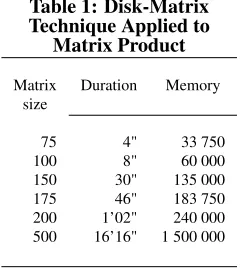
[image:10.612.319.433.269.463.2] [image:10.612.117.237.274.408.2]The DMT function and procedure are easy to implement and can be integrated in a library. The classical numerical analysis procedures can be easily changed to receive the DMT function and procedure, and the new procedures are always easily readable. The inconvenient of this technique is the time of calculation - see Tables 1 and 2. However, except the progress of the hardware, there is no really alternative, in considering the economic modelers should built more and more large-scale models, whatever the field: econometrics, micro-simulation, artificial life8, ACE9. We have assume we used the "classical" calculation algorithms, how-ever, we have to quote the recent advances of matrix multiplication techniques [8, 17, 18] which could help to economize a lot of resources10.
Table 1: Disk-Matrix Technique Applied to
Matrix Product
Matrix Duration Memory size
75 4" 33 750 100 8" 60 000 150 30" 135 000 175 46" 183 750 200 1’02" 240 000 500 16’16" 1 500 000
With 3 GHz CPU.
Table 2: Disk-Matrix Technique Applied to
Matrix Inversion
Size Durations According Methods
Pointers Disk-Matrix
10 01” 01”
20 01” 02”
50 02” 10”
80 03” 44”
100 05” 1′24” 200 - 11′38”
250 - 26′34”
500 - 180′00”
With 3 GHz CPU
8
- See [23] 9
- See the paper of L.Tesfatsion [21]. 10
- About some sophisticated algorithms see http://www.nag.co.uk or
References
[1] Almon C., "Scientific Programming with Borland’s C++Builder", Working Paper Inforum, 98-003, University of Mary-land, 1998, 16 p.
[2] Althaus M., Turbo-Pascal 6.0, Paris, Sybex, 1990, 894 p.
[3] Amman H.M., D.A.Kendrick & J.Rust (Eds), Handbook of Computational Economics, Vol.1, Amsterdam, North-Holland, 1996, 827 p.
[4] Amman H.M. & D.A.Kendrick, "Pro-gramming languages in economics",
Computational Economics, 14(1–2),
1999, pp.151–181.
[5] Borland,Turbo-Pascal Numerical Meth-ods Toolbox, Borland Press, 1987.
[6] Buda R., "SIMUL - Manuel de références et guide d’utilisation version 3.1", Mimeo GAMA, Université de Paris 10, 60 p., 1999 + Le logiciel SIMUL.
[7] ———–, "Les algorithmes de la mod-élisation : une analyse critique pour la modélisation économique", Document de recherche MODEM, Université de Paris 10, 01(44), 2001, 97 p.
[8] Cohn H. & C.Umans, "A Group-theoretic Approach to Fast Matrix Multiplication", arXiv:math.GR/0307321,Proceedings of the 44th Annual IEEE Symposium on Foundations of Computer Science, 11-14 October 2003, Cambridge, MA, IEEE Computer Society, 2003, pp.438–449.
[9] Cribari-Neto F., "C for Econometri-cians",Computational Economics, 14(1– 2), 1999, pp.135–149.
[10] Fair R., "Computational Methods for Macroeconometric Models," in
H.M.Amman, D.A.Kendrick & J.Rust (Eds.), Handbook of Computational
Economics, North-Holland, 1996,
pp.143–169.
[11] Herbert R.D., "Modelling programming languages - appropriate tools?",Journal of Economic and Social Measurement, 29(1–3), 2004, pp.321–337.
[12] Khanniche M.S. & S.H.Yong, "A Solu-tion to Memory Limit of DOS Based Large Finite Element Programs", Ad-vances in Engineering Software, 21, 1994, pp.99–112.
[13] Knuth D.E., The Art of Programming - tome 2, Seminumerical Algorithms, (Third ed.), Reading (Mass.), Addison-Wesley, 762 p., 1997.
[14] Monasse D.,Mathématiques et informa-tique - classes préparatoires aux grandes écoles scientifiques, Paris, Vuibert, Coll. Cours et travaux dirigés, 1988, 223 p.
[15] Nerlove M., "Programming languages: A short history for economists",Journal of Economic and Social Measurement, 29(1–3), 2004, pp.189–203.
[16] Press W.H., S.A.Teukolsky, W.T.Vetterling & B.P.Flannery,
Nu-merical Recipes in C++: The Art
of Scientific Computing, Cambridge, Cambridge University Press, 2002, 1002 p.
[17] Raz R., "On the complexity of matrix product", in Proceedings of the thirty-fourth annual ACM symposium on The-ory of computing, ACM Press, 2002.
[18] Robinson S., "Toward an Optimal Algo-rithm for Matrix Multiplication", SIAM News, 38(9), nov., 2005.
[19] Schink G.R., "Simulation with large econometric models: The quest for a so-lution",Journal of Economic and Social Measurement, 29(1–3), 2004, pp.135– 143.
Measurement, 29(1–3), 2004, pp.205– 259.
[21] Tesfatsion L., "Agent-based Computa-tional Economics: Growing Economies from the Bottom Up", Working Paper Iowa State university, N◦1, Dept. of Eco-nomics, 2002.
[22] Tischer M., Turbo-Pascal 5.0 & 5.5 : Programmation système, Paris, Micro-application, 1990, 823 p.