Classification of Normal and Pathological Voice using GA and SVM

Classification of Normal and Pathological Voice using

GA and SVM

V.Srinivasan

Dept of Computer Science and Engg,

Annamalai University-608002

V.Ramalingam

,

Dept of Computer Science and Engg,

Annamalai University-608002

V.Sellam*

Dept of Computer Science and Engg,

Annamalai University-608002

ABSTRACT

The analysis of pathological voice is a challenging and an important area of research in speech processing. Acoustic characteristics of voice are used mainly to discriminate normal voices from pathological voices. This study explores methods to find the ability of acoustic parameters in discrimination of normal voices from pathological voices. An attempt is made to analyze and to classify pathological voice from normal voice in children. The classification of pathological voice from normal voice is implemented using support vector machine (SVM). The normal and pathological voices of children are used to train and test the classifier. A dataset is constructed by recording speech utterances of a set of Tamil phrases. The speech signal is then analyzed in order to extract the acoustic parameters such as the Signal Energy, pitch, formant frequencies, Mean Square Residual signal, Reflection coefficients, Jitter and Shimmer. In this study various acoustic features are combined to form a feature set, so as to detect voice disorders in children based on which further treatments can be prescribed by a pathologist. A Genetic Algorithm (GA) based feature selection is utilized to select best set of features which improves the classification accuracy.

General Terms

Feature Extraction, Feature Selection, Pattern Classification

Keywords

Pitch, Formants, Jitter, Shimmer, Signal Energy, Reflection Coefficients, Genetic Algorithm, SVM.

1.

INTRODUCTION

Speech pathology is a field of the health science which deals with the evaluation of speech, language, and voice disorders. The voice disorders are caused due to defects in the speech organs, mental illness, hearing impairment, autism, paralysis, or multiple disabilities. Clinically a number of guidelines and methods are used in practice for detection of voice disorders in children. In this study an automatic classification of pathological voice disorder using acoustic features is proposed. Acoustic features, which are used to identify voice disorders, best describe the functioning and condition of various speech organs. Pitch is an attribute which represents the structure and size of the larynx and vocal folds. Pitch is closely related to frequency, but the two are not equivalent. Formants are the distinguishing or meaningful frequency components of human speech that humans require to distinguish between vowels. The formant with the lowest frequency is called f1, the second f2, and the third f3. Most

often the first two formants, f1 and f2, are enough to

disambiguate the vowel. These two formants determine the quality of vowels in terms of the open/close and front/back

dimensions. LPC is generally used for speech analysis and re-synthesis. During speech synthesis the values of the reflection coefficients are used to define the digital lattice filter which acts as the vocal tract in this speech synthesis system. In general if the energy of the speech signal is higher, then the volume of the output speech signal will also be higher. Using these acoustic features an extensive number of research are carried and various algorithms are used for extracting these features from the speech signal. The goal of the feature extractor is to characterize an object to be recognized by measurements whose values are very similar for objects in the same category and very different for the objects in different categories leading to the idea of seeking distinguishing features that are invariant to irrelevant transformations of the input. Although a large number of different methods have been proposed for detecting pitch, the autocorrelation pitch detector is still one of the most robust and reliable of all pitch detectors.

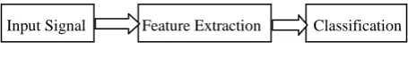
After feature extraction, a dimensionality reduction process based on Genetic algorithm is carried out to select the best feature set so that the classification of feature vectors using SVM is efficient. The patterns for training the SVM were obtained from the recordings of children voices with normal voice and children with pathological voice. Since there are different types of kernels, we are cross validating the kernels to find the best hyperparameters. The basis of SVM approach is the projection of low-dimensional training data in a higher dimensional feature space, because it is easier to separate input data. Hence SVM classifies the pathological voice from normal voice. The general process of classification is shown in Fig. 1.

Input Signal Feature Extraction Classification

Fig 1: Overview of Classification

1.1

Related Works:

on classification part rather than feature extraction [4]. [5] Compares various kernel functions and helps to identify Laryngeal disorder. [6] Evaluates the computational time and hence feature extraction is carried out using MFCC and classified using GMM. This paper deals with the extraction of acoustic parameters from the residue signal and diagnoses 21 different voice disorders [7].

2.

ACOUSTIC FEATURE EXTRACTION

2.1

Signal Energy

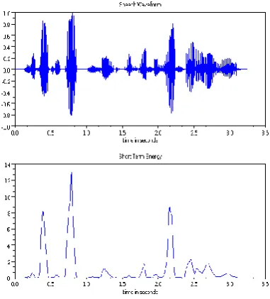
The amplitude of unvoiced segments is noticeably lower than that of the voiced segments. The higher the energy, the higher the volume of the output speech signals. The short-time energy of speech signals reflects the amplitude variation and is defined using the equation below as in [1].

 

 

1 n N

1 i E

 

 _{, (1)}

N is the length of the sample.

In order to reflect the amplitude variations in time (for this a short window is necessary), and considering the need for a low pass filter to provide smoothing, h(n) was chosen to be a hamming window powered by 2. It has been shown to give good results in terms of reflecting amplitude variations.

Fig 2: A speech signal (a) Speech Waveform (b) Short Term Energy.

In voiced speech the short-time energy values are much higher than in unvoiced speech, which has a higher zero crossing rate.

2.2

Pitch

Voiced speech signals can be considered as quasi-periodic. The basic period is called the pitch period. The average pitch frequency (in short, the pitch), time pattern, gain, and fluctuation change from one individual speaker to another. For speech signal analysis, and especially for synthesis, identifying the pitch is extremely important. A well-known method for pitch detection is given in [9]. It is based on the

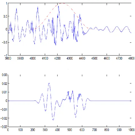
fact that two consecutive pitch cycles have a high cross-correlation value, as opposed to two consecutive speech fractions of the same length but different from the pitch cycle time. The Fig 3 below describes a vocal phoneme, in which the pitch marks are denoted in red.

The pitch detector’s algorithm can be given by the equation as below.

Fig 3: A phoneme with its pitch cycle marks (in red).

3.

PATTERN CLASSIFICATION

3.1

Support Vector Machine

In machine learning, support vector machines are supervised learning models with associated learning algorithms that

analyze data and recognize patterns, used

for classification and regression analysis. The basic SVM takes a set of input data and predicts, for each given input, which of two possible classes forms the output, making it a non-probabilistic binary linear classifier. Given a set of training examples, each marked as belonging to one of two categories, an SVM training algorithm builds a model that assigns new examples into one category or the other. An SVM model is a representation of the examples as points in space, mapped so that the examples of the separate categories are divided by a clear gap that is as wide as possible. New examples are then mapped into that same space and predicted to belong to a category based on which side of the gap they fall on. A support vector machine constructs a hyperplane or set of hyperplanes in a high- or infinite-dimensional space, which can be used for classification, regression, or other tasks. Intuitively, a good separation is achieved by the hyperplane that has the largest distance to the nearest training data point of any class (so-called functional margin), since in general the larger the margin the lower the generalization error of the classifier.

A linear support vector machine is composed of a set of given support vectors z and a set of weights w.The computation for the output of a given SVM with N support vectors z1, z2 ….,zN

and weights w1,w2,…….,wN is then given by:

; ǁ

(2)

Fig 4: Principle of SVM

4.

PROPOSED METHODOLOGY

The speech from the pathological voiced children and normal children was recorded. They are trained to utter same set of phrases and the silences in between speech utterances are clipped off using a silence removal algorithm.

Fig 5: System overview for classifying the normal and pathological voice.

4.1

Silence Removal

Silence removal is considered to be one of the efficient dimensionality reduction processes. The signal energy and spectral centroid are used for silence removal in speech signal. The segments are decided based on the threshold value, which is extracted from the feature sequences of the input signal. Signal Energy of the ith frame is defined using the formula

 

 

n i x N

1 n N 1 i E

  

, (4)

N is the length of the sample.

The spectral centroid, Ci is defined as the center of gravity of

the spectrum.



  

 

 

i x N

1 k

k i x 1 k N

1 k i C

 

  

 , (5)

where

x

4.2

Windowing

Speech is non-stationary signal where properties change quite rapidly over time. This is completely natural and nice thing but makes the use of DFT or autocorrelation as such impossible. For most phonemes the properties of the speech

remain invariant for a short period of time (5-100 ms). Thus for a short window of time, traditional signal processing methods can be applied relatively successfully. Most of speech processing in fact is done in this way: by taking short windows (overlapping possibly) and processing them. The short window of signal like this is called frame. In implementation view, the windowing corresponds to what is understood in filter design as window-method: a long signal (of speech for instance or ideal impulse response) is multiplied with a window function of finite length, giving finite length weighted (usually) version of the original signal and is shown below in Fig. 6.

Fig 6: (a) Original Signal (b)Windowed Signal.

4.3

Fundamental Frequency Estimation

A pitch detection algorithm (PDA) is an algorithm designed to

estimate the pitch or fundamental frequency of

a quasiperiodic or virtually periodic signal, usually a digital recording of speech or a musical note or tone. Fundamental Frequency (f0) or pitch voice corresponds perceptually to the number of times per second the vocal folds come together during phonation. Fundamental frequency has long been difficult parameter to reliably estimate from the speech signal. Previously it was neglected for number of reasons, including large computational burden required for accurate estimation, the concern that unreliable estimation would be a barrier achieving high performance, and the difficulty in characterizing complex interactions between and suprasegmental phenomena. The time-domain pitch period estimation techniques use auto-correlation function (ACF). The basic idea of correlation-based pitch tracking is that the correlation signal will have a peak of large magnitude at a lag corresponding to the pitch period. The autocorrelation computation is made directly on the waveform and is a fairly straightforward computation [1].

The information about pitch period 'To'is more pronounced in

the autocorrelation sequence of voiced speech compared to the speech segment itself. Since autocorrelation sequence is symmetric with respect to zero lag, only positive lag values are considered. The 'To' information is more pronounced in

the autocorrelation sequence compared to speech. By that, the Silence

Removal

Feature Selection using GA Classification

by SVM

Windowing Feature

Extraction

second largest peak is the autocorrelation sequence, represents pitch T0 andcan be picked up easily by a simple peak picking

algorithm compared to finding 'To' from the speech segment

itself. Hence autocorrelation method is preferred over other direct methods of pitch estimation from speech.

Autocorrelation function for a signal x(n) is computed as given in [1]:

The autocorrelation function of a signal is basically a (non-invertible) transformation of the signal which is useful for displaying structure in the waveform. Thus, for pitch detection, if we assume x(n) is exactly periodic with period P, i.e. x(n)=x(n+P) for all n, then the autocorrelation function

Øx(m) is also periodic with the same period,

.

4.4

Formant Estimation

Linear Predictive Coding analyzes the speech signal by estimating the formants, removing their effects from the speech signal, and estimating the intensity and frequency of the remaining buzz. The process of removing the formants is called inverse filtering, and the remaining signal after the subtraction of the filtered modelled signal is called the residue. A formant or resonance of the vocal tract above the vocal folds is a frequency region that will strongly pass energy in that frequency region if it receives energy at those frequencies from the glottal source (glottal flow). The formant frequencies depend upon the size and shape of the vocal tract. In autoregressive coding of speech, it is essential that the LPC model contain accurate information about the first three formants; specifically, that the LPC spectrum should reproduce the correct formant frequencies and the corresponding bandwidths. The modified linear predictive coder (MLPC) is superior to the widely used linear predictive coder (LPC) when the data frames are short. Perception of these syllables critically depends on accurate detection of the rapid frequency changes in the first milliseconds of voicing (formant transitions). Inaccurate detection of these formant transitions inevitably interferes with the identification of the phonological cues that are typical for spoken language. The resonant(formant) frequency of a uniform tube, which is a model of the vocal tract [4] is given by the equation below:

Where

Fn nth formant frequency[Hz]

c sound velocity [m/s] L vocal tract Length[m].

The aim of linear prediction is to estimate the transfer function of the vocal tract from the speech. The signal model can be defined as:

Where NLP, αLP and e(n) represent, respectively, the number

of coefficients in the model the linear prediction coefficients and the error in the model. The above equation can be written in Z-transform notation as a linear filtering operation:

4.5

Jitter Estimation

Jitter deals with varying loudness in the voice. Jitter is said to be the interval between the maximum effects or minimum effects of a signal characteristic that changes regularly in time. The average absolute difference between consecutive periods is expressed as in [8]:

Where Ti are the extracted F0 period lengths and N is the

number of extracted F0 periods.

Jitter (relative) is the average absolute difference between consecutive periods, divided by the average period and is expressed as a percentage [8]:

4.6

Shimmer Estimation

Shimmer deals with a frequent back and forth change in amplitude in the voice. . The average absolute base-10 logarithm of the difference between the amplitudes of consecutive periods, multiplied by 20 as in [8]:

Where Ai is the extracted peak-to-peak amplitude data and N

is the number of extracted fundamental frequency periods.

Shimmer (relative) is defined as the average absolute difference between the amplitudes of consecutive periods, divided by the average amplitude, expressed as in [8]:

4.7

Reflection Coefficients

A reflection coefficient calculated from the cross-sectional areas of vocal tubes expresses the rate of reflection.. Let the cross-sectional area of the left tube be Sn and of the right tube

be Sn+1. The reflection coefficient kn is defined as follows:

4.8

Feature Selection Using GA

The feature selection deals with the task of selecting the best feature set which reduces the classifier training time and as well as increase the classification accuracy. From a given set of the features, the feature selection algorithm selects a subset of size m which increases the classification accuracy [10]. If the size of the feature set is m then there will be 2m _possible

feature subsets. The selection of best feature subset can be viewed as a combinatorial optimization problem and is solved using Genetic Algorithms as proposed in [11]. Each speech sample is processed by the above mentioned techniques in the literature and acoustic features are extracted. In the representation method used in this study, the chromosome is

(8)

Jitter (absolute) = | (10)

Jitter (relative)= (11)

Shimmer (relative) = (13)

(14)

(6)

= (7)

represented using a bit string whose length is same as the number of eigenvectors. For each feature vector one bit in the string is associated. If the ith bit is 1, then the ith feature vector is selected, otherwise, that component is ignored. Thus each chromosome represents a different feature subset. The main aim of using the feature selection algorithm is to use fewer features to attain the same or better classification accuracy. Therefore, the fitness evaluation contains two terms: (i) accuracy and (ii) number of features used. The fitness function is calculated as proposed in [12]

fitness = 104 Accuracy + 0.4 × Zeros (15)

where Accuracy is the classification accuracy rate that an individual feature set achieves, and Zeros is the number of zeros in the chromosome. If the accuracy is higher, then the fitness will also be higher.

4.9

Classification

The SVM algorithm can construct a variety of learning machines by use of different kernel functions [4]. Three kinds of kernel functions are usually used

4.9.1 Linear Kernel

The Linear kernel is the simplest kernel function. It is given by the common inner product <x,y> plus an optional constant c. Kernel algorithms using a linear kernel are equivalent to their non-kernel counterparts.

(16)

4.9.2 Polynomial Kernel

The polynomial kernel is a non-stationary kernel. It is well suited for problems where all data is normalized.

(17)

4.9.3 Gaussian Kernel

Gaussian kernel is one of the most versatile kernels. The width parameter of the Gaussian kernel controls the flexibility of the resulting classifier.

5.

EXPERIMENTS AND RESULTS

The experiments were performed using the recorded speech samples from the children. The database contains speech samples 10 distinct subjects (5 normal, 5 pathological children). All the speech samples were recorded in noise free environment using a microphone array. Each speech sample is pre-processed using a silence removal algorithm and a windowing technique. Using Autocorrelation method the fundamental frequency is estimated, and Linear predictive analysis is used to extract the formant frequencies F1 and F2. The two first formants, f1 and f2, are enough to disambiguate

the normal and pathological voices. Since the number of formants is same for all the utterances the peaks of the formant frequencies are found using a magnitude threshold based peak detection algorithm. The feature vector is constructed using the peaks of Formant frequencies, average pitch period, the signal energy, mean square residual signal, reflection coefficients, jitter and shimmer. Combining all these feature vectors forms a 16 coefficient feature set. Using the Genetic algorithm based feature selection method the

optimal feature subset is extracted using the fitness function. The classifier is trained and tested with feature set and the classification accuracy is calculated using the formula.

Classification Accuracy = (Total No. of samples taken – No. of samples misclassified) / Total No. of samples taken

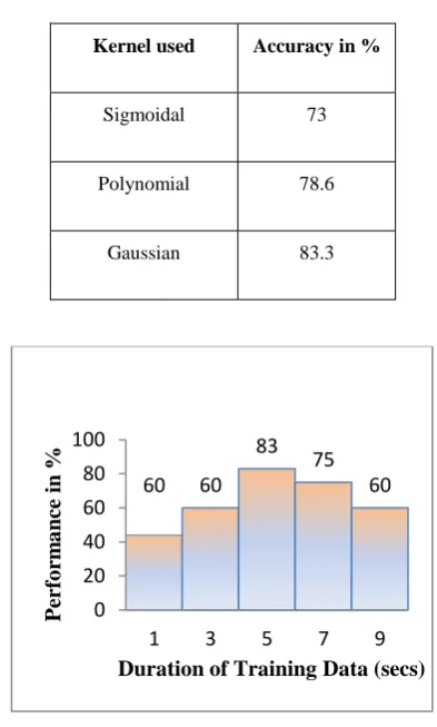
The Table 1 shows the classification accuracy of the various kernels used for classification. Of all the kernels used in this study the Gaussian Kernel shows better performance in terms of classification accuracy.

Table 1: Classification Performance Using Different Kernel Functions.

Kernel used Accuracy in %

Sigmoidal 73

Polynomial 78.6

Gaussian 83.3

Fig: 7 Performance of Gaussian Kernel

Fig.7 infers that the performance is optimum when the speech signal duration is around 5 seconds.

6.

CONCLUSION

In this paper several acoustic techniques for extracting different acoustic parameters and providing a hybrid approach of feature extraction is being presented. A feature selection is done for selecting the best feature set. The feature set is then classified using 3 different kernels of SVM classifier. Out of those kernels “Gaussian kernel” provides better classification accuracy when compared with others. The future work will be based on extracting different feature sets and comparing those with the present features. Considering all the features, a combined feature set may be constructed for measuring their performance. Further this feature set will be used to implement different classification models so as to compare with SVM kernel functions.

60 60

83 75

60

0 20 40 60 80 100

1 3 5 7 9

Per

fo

rm

a

n

ce

in

%

Duration of Training Data (secs)

ACKNOWLEDGEMENTS

The authors would like to thank S.Palanivel and P.Dhanalakshmi for providing the lab facilities of AICTE funded project (RPS) and UGC funded project.

REFERENCES

[1] L.Salhi, M.Talbi, A.Cherif “Voice Disorders Identification Using Hybrid Approach: Wavelet Analysis and Multilayer Neural Networks”, World Academy of Science, Engineering and Technology 2008.

[2] Awrence R.Rabiner,”On the Use of Autocorrelation Analysis for Pitch Detection”, IEEE Transactions on Acoustics, Speech, and Signal Processing, Vol ASSP-25, No.1, Feb 1977.

[3] Pend Ce, Xu Qiujing, Wan Baikun, Chen Wenxi,” Pathological Voice Classification Based on Features Dimension Optimization”, Transactions of Tianjin University,Vol.13,No.6,Dec 2007.

[4] P.Dhanalakshmi*,S.Palanivel,V.Ramalingam,”Classifica tion of Audio Signals Using SVM and RBFNN”, Expert Systems with Applications 36(2009) 6069-6075 .

[5] Evaldas Vaiciukynas, Adas Gelzins, Marija Bacauskiene, Antanas Verikas,Aurelija Vegiene,” Exploring Kernels in SVM-Based Classification of Larynx Pathology from Human Voice”,Department of Electrical and Control Instrumentation, Kaunas University of Technology, Lithuania.

[6] Pravena D, Dhivya S,Durga DeviA,”Pathological Voice Recognition for Vocal Fold Didease”, International

Journal of Computer Applications(0975-888), Volume 47-No.13,June 2012

[7] Marcelo de Oliviera Rosa*,Jose Carlos Pereira, and Marcos Grellet,” Adaptive Estimation of Residue Signal for Voice Pathology Diagnosis” IEEE Transactions on Biomedical Engineering,Vol.47, No.1,Jan 2000.

[8] Mireia Farra, Javier Hernando, Pascual Ejarque,” Jitter and Shimmer Measurements for Speaker Recognition”, TALP Research Center, Department of Signal Theory and Communicati0ons, Universitat Politecnica de Catalunya, Barcelona,Spain.

[9] L.R.Rabiner, R.W.Schafer,”Digital Processing of Speech Signals”

[10]Yoav Meden, Eyal Yair, and Dan Chazan,” Super Resolution Pitch Determination of Speech Signals”, IEEE transactions on Signal Processing,Vol.39,No.1,Jan 1991.

[11]Ahmed Al-Ani,” Ant Colony Optimization for Feature Subset Selection”, Proceedings of World Academy of Science, Engineering and Technology, Feb 2005, Vol.4 ISSN1307-6884.

[11] O.Ludwig, U.Nunes,” Novel Maximum Margin Training algorithms for Supervised Neural Networks”, IEEE Transactions on Neural Networks,vol.21,issue 6,pp.972-984,Jun.2010.

[12] Z.Sun, X.Yuan, G.Bebis, S.Louis,” Neural Network Based Gender Classification Using Genetic Eigen Feature Extraction”, IEEE International Joint Conference