Implementation and Analysis of the Bee Colony Optimization algorithm for Fault based Regression Test Suite Prioritization

Implementation and Analysis of the Bee Colony

Optimization algorithm for Fault based Regression Test

Suite Prioritization

Arvinder Kaur

University School of Information Technology Guru Gobind Singh Indraprastha University

Sec 16-c, Dwarka, Delhi

Shivangi Goyal

University School of Information Technology Guru Gobind Singh Indraprastha University

Sec 16-c, Dwarka, Delhi

ABSTRACT

Regression Testing is an important maintenance phase testing activity. The importance of this activity lies in the fact that it imparts confidence and accuracy in the modified code, as well as keeps a check on the unmodified parts, if they are affected or not. But there is a severe requirement to reorder the development testing test suite because of the constrained software development budget, time and effort. So techniques have to be developed to prioritize test cases to reduce budget, time and effort constraints effectively. In this paper implementation and analysis of an existing fault based regression test suite has been done. The prioritization algorithm is based on the nature inspired algorithm called Bee Colony Optimization (BCO) algorithm. The algorithm is a two step procedure which maps the food foraging behavior of scout bee and forager bee one after the other to reach to the solution. The analysis of the examples using the code developed indicates that the two step BCO algorithm is able to produce results which are comparable to optimal results.

General Terms

Regression Testing, Implementation, Analysis.

Keywords

Fault based Test Suite Prioritization, Bee Colony Optimization (BCO).

1.

INTRODUCTION

In SDLC, the maintenance phase is a phase that extends from 10 to 15 years. In these maintenance years the software undergoes a number of editions/omissions/up-gradations. These changes are like mini-softwares in which the SDLC are executed but in budget, time and effort constraints. So, while testing software‟s reformed version we cannot use the same old development testing process, since for development testing there is ample amount of budget, time and effort sanctioned. So there is a requirement to reorder or prioritize the test suite so that the relevant ones are executed first within permissible budget and time constraints. There are many ways to prioritize the regression test suites. Some of them being Fault based prioritization [1], code coverage based prioritization [2], statement coverage based prioritization [4], branch coverage based prioritization [4], and failure rates

based prioritization [3].

In fault based regression test suite prioritization in [1] the fault seeding method has been used to insert faults into the existing code. Then the test cases are ordered according to the number of faults detected by a test case. Hence test cases with more fault detection capabilities become the first ones to fall into the ordering.

In the year 2011 kaur et al proposed a BCO algorithm for fault based regression test suite prioritization. The algorithm proposed in this paper was implemented but the implementation was not analyzed. The [1] paper has been used as s basis for this paper. In this paper the algorithm has been analyzed.

2.

BEE COLONY OPTIMIZATION

Bee Colony Optimization is a nature inspired optimization technique in which the food foraging behavior of honey bees is mapped to find solution to the problem in hand. Bee colony system can also be thought of as a Particle Swarm Optimization in which the agents are bees. Bee colony has been considered as an excellent example of team work, labor distribution, coordinated message passing, synchronization etc. In Bee Colony the worker bee‟s food foraging behavior is studied and mapped to find solution to the problem in hand.

The proposed algorithm is a two step algorithm in which the scout‟s and forager‟s food foraging behaviors have been mapped step by step to formalize the solution to the fault based prioritization.

3.

BCO ALGORITHM

In the proposed BCO technique in [1] the test cases are prioritized in such a manner so as to achieve maximum fault coverage within minimum execution time. To ensure that all the faults are covered by the test cases selected in the prioritized ordering we use mutation testing. In this we deliberately alter a program‟s code, then re-run a suite of valid test cases against the mutated program. A good test will detect the change (fault) in the program and fail accordingly.

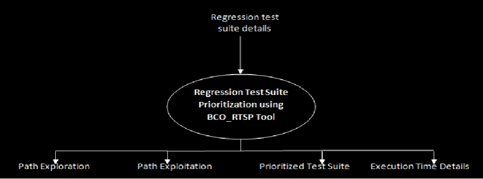
Thus, the proposed algorithm‟s effectiveness is measured using mutation testing. The block diagram of the BCO

Fig 1: Block Diagram of BCO_RTSP tool.

4.

IMPLENEMTATION DETAILS

The algorithm has been coded as “BCO_RTSP” which is a C++ code compiled using TURBO C++ compiler, implemented on an Intel core 2 duo Processor T8100 at 2.10 Ghz (2 Gb RAM).

The BCO tool is made up of 10 modules having 3 global functions, 2 global structures, 12 global temporary variables. Following is the explanation of a few modules which were implemented:

1. BCO_Init()

It is an initialization module for the „bee‟ structure. It is called before the start of the BCO algorithm.

2. TS_Input()

This module inputs the regression test suite details from the user which would be prioritized by the BCO algorithm.

3. BCO()

This module is the heart of the BCO_RTSP tool. It is called from the main() module and it gives the prioritized test suite as output. This module is executed with the initial bee values initialized by the BCO_Init() module. In this module path exploration, path exploitation, final prioritized path display processes are executed.

Screenshots for the processing and output of the BCO_RTSP tool have been shown in fig 2 and 3. In order to compute the efficiency of the BCO_RTSP tool, it was executed on 5 examples taken from [1]. The BCO_RTSP tool was run 10 times on each example and the outcome of each execution was recorded. All the details of execution and the outcomes of each execution are presented in detail in the following Analysis section.

Fig 3: Screenshot 2 of BCO_RTSP tool.

5.

ANALYSIS

In the proposed BCO technique the test cases were prioritized so as to achieve maximum or total fault coverage. Mutation testing was used to ensure that all the faults have been covered by the test cases selected in the prioritized ordering.

5.1. Example 1

The problem taken is “college program for admission in courses”. The problem specification is available at website http://www.planet-source-code.com. In example 1 a test suite with 9 test cases covering a total of 5 faults.

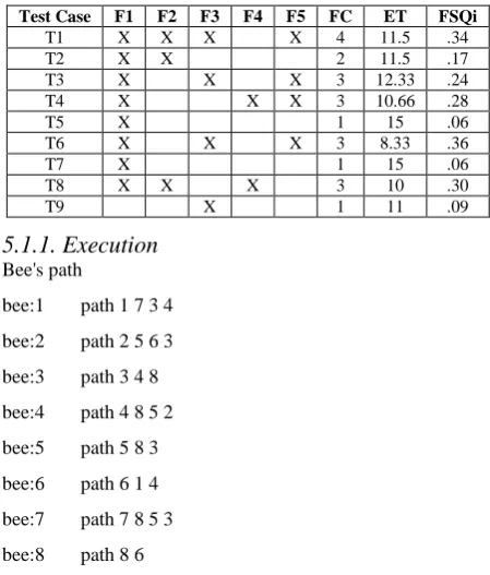
The input test suite contains 9 test cases with default ordering {T1, T2, T3, T4, T5, T6, T7, T8, T9}, the faults covered (FC) by each test case, the execution time (ET) required by each test case in finding faults and food source quality (FSQ) are as shown in Table 1.

Table 1. Test cases with the faults covered, execution time and food source quality

Test Case F1 F2 F3 F4 F5 FC ET FSQi

T1 X X X X 4 11.5 .34

T2 X X 2 11.5 .17

T3 X X X 3 12.33 .24 T4 X X X 3 10.66 .28

T5 X 1 15 .06

T6 X X X 3 8.33 .36

T7 X 1 15 .06

T8 X X X 3 10 .30

T9 X 1 11 .09

5.1.1. Execution

Bee's path

bee:1 path 1 7 3 4 bee:2 path 2 5 6 3 bee:3 path 3 4 8 bee:4 path 4 8 5 2 bee:5 path 5 8 3 bee:6 path 6 1 4 bee:7 path 7 8 5 3 bee:8 path 8 6

bee:9 path 9 3 4 2 1 4 ex. time: 22.16 6 2 ex. time: 32.989998 8 4 3 ex. time: 20.66 8 4 ex. time: 20.66 8 3 ex. time: 22.33 6 1 4 ex. time: 30.49 8 3 ex. time: 22.33 6 8 ex. time: 18.33 4 3 2 ex. time: 34.489998 FINAL PATH : 6 8

exc. time : 18.33

5.1.2. Analysis

Example 1, presented in section 5.1. was executed 10 times for the given test suite. There were a bunch of varying results for the same which had the optimal result also. The optimal test suite prioritization order for example 1 is T6 T8 with execution time of 18.33 units, which was found out to be appearing 6 times. The code produced other outputs also which have been shown below and have also been summarized in Table 2.

Table 2. Summary of outcomes of 10 runs of example 1.

S. No

BCO ORDER

EXECUTIO N TIME

IS ORDER OPTIMAL?

Y/N

NO. OF TIMES OF

THIS OUTCOME

1 T6, T8 18.33 Y 5

2 T1, T8 21.50 N 1

3 T1, T4 22.16 N 2

4 T8, T3 22.33 N 1

5 T6, T4 18.99 N 1

5.2. Example 2

The input test suite contains 5 test cases with default ordering {T1, T2, T3, T4, T5}, the faults covered (FC) by each test case, the execution time (ET) required by each test case in finding faults and food source quality (FSQ) are as shown in Table 3.

Table 3. Test cases with the faults covered, execution time and food source quality.

Test Case

F1 F2 F3 F4 F5 FC ET FSQi

T1 x x x 3 12.2 .2459

T2 x 1 10 .10

T3 x x x 3 10.67 .28

T4 x 1 7 .14

T5 x x x x 4 9.97 .40

5.2.1. Execution

Bee's path bee:1 path 1 2 bee:2 path 2 4 bee:3 path 3 4 bee:4 path 4 1 bee:5 path 5 3 3 1 ex. times: 23.07 4 2 ex. time: 17 3 ex. time: 10.67 1 4 ex. time: 19.4 5 3 ex. time: 20.639999 FINAL PATH: 5 3

exc. time: 20.639999

5.2.2. Analysis

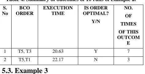
Example 2 was executed 10 times for the given test suite. There were a bunch of varying results for the same which had the optimal result also. The optimal test suite prioritization order for example 2 is T5 T3 with execution time of 20.63 units, which was found out to be appearing 7 times. The code produced other outputs also which have been shown below and have also been summarized in Table 4.

Table 4. Summary of outcomes of 10 runs of example 2.

S. No

BCO ORDER

EXECUTION TIME

IS ORDER OPTIMAL?

Y/N

NO. OF TIMES OF THIS OUTCOM

E

1 T5, T3 20.63 Y 7

2 T5,T1 22.17 N 3

5.3. Example 3

The problem in taken example 3 is “the triangle problem”. The problem specification is available in [81]. In this example a test suite has been developed which consisted of 12 test cases. The input test suite contains 12 test cases with default ordering {T1, T2, T3, T4, T5, T6, T7, T8, T9, T10, T11,

T12}, the faults covered (FC) by each test case and the execution time (ET) required by each test case in finding faults are as shown in Table 5.

Table 5. Test cases with the faults covered, execution time and food source quality.

Test Case

F1 F2 F3 F4 F5 F6 FC ET

T1 X X X 3 5

T2 X X X X 4 2 T3 X X X X 4 3 T4 X X X X 4 4 T5 X X X X X 5 5 T6 X X X X 4 6

T7 X X X 3 4

T8 X X X X 4 5 T9 X X X X X 5 8 T10 X X X X 4 4

T11 X X X 3 3

T12 X X X X 4 2

5.3.1. Execution

5.3.2. Analysis

Example 3 was executed 10 times for the given test suite. There were a bunch of varying results for the same which had the optimal result also. The optimal test suite prioritization order for example 3 is T5 T2 with execution time of 7 units, which was found out to be appearing 7 times. The code produced other outputs also which have been shown below and have also been summarized in Table 6.

5.4. Example 4

The problem taken is “the quadratic equation problem”. The problem specification is available [5]. In this example a test suite has been developed which consisted of 18 test cases. For simplified explanation of the working of the algorithm, a test suite with 9 test cases is considered in it, covering a total of 9 faults.

Table 6. Summary of outcomes of 10 runs of example 3.

S. No

BCO ORDER

EXECUTION TIME

IS ORDER OPTIMAL?

Y/N

NO. OF TIMES OF

THIS OUTCOME

1 T5, T7 9 N 1

2 T2, T5 7 Y 6

3 T2, T9 10 N 1

4 T12, T5 7 Y 1

5 T3, T5 8 N 1

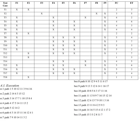
The input test suite contains 9 test cases with default ordering {T1, T2, T3, T4, T5, T6, T7, T8, T9, T10, T11, T12, T13, T14, T15, T16, T17, T18}, the faults covered (FC) by each test case, the execution time (ET) required by each test case in finding faults and are as shown in Table 7.

Table 7. Test cases with the faults covered, execution time and food source quality.

Test Case

F1 F2 F3 F4 F5 F6 F7 F8 F9 FC ET

T1 X X 2 3

T2 X X X 3 5

T3 X X X X 4 2

T4 X X X X 4 6

T5 X X X X 4 3

T6 X X X X 4 4

T7 X X 2 2

T8 X X X X X 5 4

T9 X X X X X 5 7

T10 X X X X X 5 3

T11 X X X X X 5 2

T12 X X X X X 1 7

T13 X 1 3

T14 X X X X 4 5

T15 X X X X X 5 6

T16 X X X X X 5 3

T17 X X X X X 5 4

T18 X 1 1

5.4.1. Execution

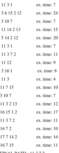
bee:1 path 1 5 10 12 11 3 9 6 16 bee:2 path 2 14 6 3 15 12 bee:3 path 3 14 17 7 1 10 15 8 4 bee:4 path 4 17 5 14 11 13 2 bee:5 path 5 12 14 2

bee:6 path 6 3 14 15 11 16 12 4 1 bee:7 path 7 9 10 14 11 3 2

bee:16 path 16 6 2 4 8 9 13 7 1 bee:17 path 17 2 7 4 9 14 bee:18 path 18 15 9 4 16 6 7 12 5 11 3 1 ex. time: 7 3 6 15 2 12 ex. time: 24 3 10 7 ex. time: 7 11 14 2 13 ex. time: 15 5 14 2 12 ex. time: 20 11 3 1 ex. time: 7 11 3 7 2 ex. time: 11 11 12 ex. time: 9 3 16 1 ex. time: 8

11 3 ex. time: 4

11 7 15 ex. time: 10

3 10 7 ex. time: 7

11 3 2 13 ex. time: 12 16 15 1 2 ex. time: 17 11 3 7 2 ex. time: 11

16 7 2 ex. time: 10

17 7 14 2 ex. time: 16 16 7 15 ex. time: 11 FINAL PATH : 11 3 7 2 exc. time: 11

5.4.1. Analysis

Example 4 was executed 10 times for the given test suite. There were a bunch of varying results for the same which had the optimal result also. The optimal test suite prioritization order for example 4 is T11 T13 T7 T2 with execution time of 11 units, which was found out to be appearing 3 times. The code produced other outputs also which have been shown below and have also been summarized in Table 8.

Table 8. Summary of outcomes of 10 runs of example 4.

S. No BCO ORDER EXECUTION TIME IS ORDER OPTIMAL? Y/N NO. OF TIMES OF THIS OUTCOME

1 T10, T15, T2,

T13

17 N 1

2 T3, T10, T2, T7

12 N 1

3 T11, T3, T7, T2

11 Y 3

4 T3, T16, T7, T2

12 N 1

5 T11, T7, T14, T2

14 N 1

6 T8, T18, T14, T2

15 N 1

7 T3, T17, T1, T2

14 N 1

8 T11, T3, T2, T13

12 N 1

5.5. Example 5

The problem taken is “the railway ticketing system”. The problem specification is available at website http://www.planet-source-code.com. In this example a test suite has been developed which consisted of 35 test cases. For simplified explanation of the working of the algorithm, a test suite with 9 test cases is considered in it, covering a total of 5 faults.

The input test suite contains 14 test cases with default ordering {T1, T2, T3, T4, T5, T6, T7, T8, T9, T11, T12, T13, T14}, the faults covered (FC) by each test case, the execution time (ET) required by each test case in finding faults are as shown in Table 9.

Table 9. Test cases with the faults covered, execution time and food source quality.

Test Case F 1 F 2 F 3 F 4 F 5 F 6 F 7 F 8 F 9 F 1 0 F C ET

T1 X 1 8

T2 X X X X 4 12

T3 X X X X X X 6 16 T4 X X X X X X X 7 18

T5 X X X 3 16

T6 X X X 3 14

T7 X X X 3 15

T8 X X X 3 12

T9 X X X X 4 13

T10 X X X X 4 15

T11 X X X X 4 13

T12 X X X X 4 14

T13 X X X X 4 13

5.5.1. Execution

Bee's path

bee:1 path 1 6 13 10 8 12 4 bee:2 path 2 11 6 9 4 13 8 bee:3 path 3 11 13 10 5 1 4 bee:4 path 4 2 13 12 5 11 8 bee:5 path 5 9 6 10 13 8 12 bee:6 path 6 9 13 8 7 4 2 bee:7 path 7 5 9 12 13 4 11 bee:8 path 8 2 10 5 11 4 12 bee:9 path 9 5 1 12 4 13 6 bee:10 path 10 4 8 1 2 3 bee:11 path 11 13 2 7 9 4 1 bee:12 path 12 7 10 9 6 8 4 bee:13 path 13 2 1 8 10 4 3 bee:14 path 14 9 10 12 6 8 11

4 13 ex. time: 31

4 2 9 ex. time: 43 4 3 11 ex. time: 47 4 2 11 ex. time: 43

9 13 ex. time: 26

4 2 9 ex. time: 43 4 9 13 ex. time: 44 4 2 11 ex. time: 43 4 9 13 ex. time: 44

4 3 10 ex. time: 49

4 2 9 ex. time: 43

4 9 12 ex. time: 45

4 3 13 ex. time: 47

14 ex. time: 13

FINAL PATH : 4 3 11 exc. time: 47

5.5.2. Analysis

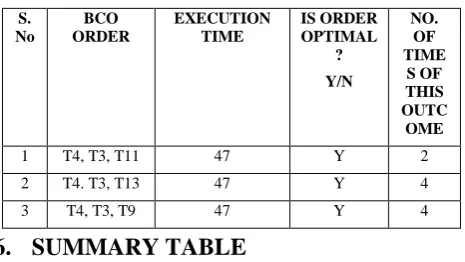
Example 5 was executed 10 times for the given test suite. There were a bunch of varying results for the same which had the optimal result also. The optimal test suite prioritization order for example 5 is T4 T3 T13 with execution time of 47 units, which was found out to be appearing 10 times. The code produced other outputs also which have been shown below and have also been summarized in Table 10

Table 10 Summary of outcomes of 10 runs of example 5.

S. No

BCO ORDER

EXECUTION TIME

IS ORDER OPTIMAL

? Y/N

NO. OF TIME

S OF THIS OUTC OME

1 T4, T3, T11 47 Y 2 2 T4. T3, T13 47 Y 4

3 T4, T3, T9 47 Y 4

6.

SUMMARY TABLE

The proposed BCO algorithm has been analyzed by running it 10 times a for particular example. We compute the Efficiency (EF) and %Savings (%S) of the proposed algorithm using following formulas:

Table 11. Summary of outcomes of 10 runs of 5 examples of fault coverage.

EXAM PLE

NO. OF TEST CASES

NO. OF FAULTS

BCO ORDER ET

NO. OF RUNS

NO.OF OPTIMAL RUNS

EFFICIEN CY %

%SAVING S

1 9 5 T6, T8 18.33 10 5 50 77.77

2 5 5 T5, T3 20. 10 7 70 60

3 12 6 T5, 52 7 10 7 70 83.33

4 18 9

T11, T13,

T7,T2 11 10 3 30 77.77

5 14 10

T4, T3,

Fig 4: Chart depicting EF of examples of fault coverage

Fig 5: Chart depicting %S in test suite of examples of fault coverage.

The values of EF and %S for the various examples discussed in section 5 have been computed and tabulated in table 11. Fig 4 and 5 gives the plots of the EF and %S for the same examples.

7.

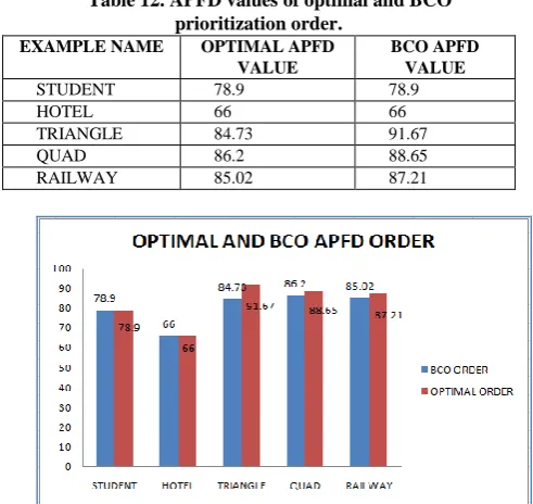
For the examples mentioned in section 5 we have computed APFD, Average Percentage of Faults Detected [5] for the BCO order and the Optimal order, the values for which are given in table 12.

APFD =

Where,

T - The test suite under evaluation

m - The number of faults contained in the program under test P

n - The total number of test cases in and

TFi - The position of the first test in T that exposes ith fault. The results obtained for the examples explained above have been plotted in APFD charts in Fig. 6. These show that the APFD values for the prioritization achieved using the proposed BCO algorithm are comparable to that obtained with the optimum ordering. The APFD values obtained for the BCO orderings for various examples of fault coverage

have been compared with the optimal orderings APFD values. Plots have also been drawn for the same.

Table 12. APFD values of optimal and BCO prioritization order.

EXAMPLE NAME OPTIMAL APFD VALUE

BCO APFD VALUE

STUDENT 78.9 78.9

HOTEL 66 66

TRIANGLE 84.73 91.67

QUAD 86.2 88.65

RAILWAY 85.02 87.21

Fig 6: APFD chart for optimal and BCO orders

8.

CONCLUSION AND FUTURE WORK

The BCO Algorithm for maximum fault coverage have been implemented and analyzed on 5 examples. It has been found out that BCO is a very efficient technique for regression test suite prioritization. The analysis work done on the examples of fault coverage shows encouraging results. The percentage savings of test cases is atleast 60% which is a remarkable reduction in the test suite size. However, the efficiency of the algorithm ranges between 30-100 %, which could be improved. Also, The APFD values of BCO order are comparable to the optimal order values. All these factors

indicate that the BCO technique could be used to prioritize the regression test suite.

REFERENCES

[1] Kaur, A. and Goyal, S., 2011. A Bee Colony Optimization Algorithm for Fault Coverage Based Regression Test Suite Prioritization, IJAST, Vol. 29(3), pp.:17-29, April 2011.

[2] Kaur, A. and Goyal, S., 2011. A Bee Colony Optimization Algorithm for Code Coverage Test Suite Prioritization. IJEST, Vol.3(4), pp.:2786-2795.April 2011.

[3] Rothermel, G. Untch, R. H., Chu, C., and Horrold, M. J., 1999. Test Case Prioritization: An Empirical Study,

Proceedings of the International Conference on Software Maintenance, pp.: 179-188, September 1999.

[4] Walcott , K. R.,So, M. L., Kapfhammer, G. M., and Roos, R. S.,2006. Time aware test suite prioritization, ISSTA, pp.: 1-11, 2006.