An Electrothermal Model Based Adaptive Control of Resistance Spot Welding Process

http://dx.doi.org/10.4236/ica.2015.62014

An Electrothermal Model Based Adaptive

Control of Resistance Spot Welding Process

Ziyad Kas, Manohar Das

Department of Electrical and Computer Engineering, Oakland University, Rochester, USA Email: [email protected], [email protected]

Received 26 February 2015; accepted 18 May 2015; published 22 May 2015

Copyright © 2015 by authors and Scientific Research Publishing Inc.

This work is licensed under the Creative Commons Attribution International License (CC BY). http://creativecommons.org/licenses/by/4.0/

Abstract

Resistance Spot Welding (RSW) is a process commonly used for joining a stack of two or three metal sheets at desired spots. The weld is accomplished by holding the metallic workpieces to-gether by applying pressure through the tips of a pair of electrodes and then passing a strong electric current for a short duration. Inconsistent weld and insufficient nugget size are some of the common problems associated with RSW. To overcome these problems, a new adaptive control scheme is proposed in this paper. It is based on an electrothermal dynamical model of the RSW process, and utilizes the principle of adaptive one-step-ahead control. It is basically a tracking controller that adjusts the weld current continuously to make sure that the temperature of the workpieces or the weld nugget tracks a desired reference temperature profile. The proposed con-trol scheme is expected to reduce energy consumption by 5% or more per weld, which can result in significant energy savings for any application requiring a high volume of spot welds. The design steps are discussed in details. Also, results of some simulation studies are presented.

Keywords

Resistance Spot Welding, Adaptive Control, Nugget Formation, Energy Saving

1. Introduction

[image:2.595.208.388.90.268.2]

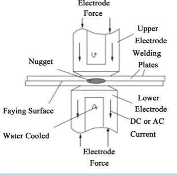
Figure 1. Resistance spot welding system.

there. Depending on the thickness and type of material, welding current ranges from 1,000 to 20,000 amperes or more, while the voltage typically is between 1 and 30 volts [2].

A Resistance Spot Welding cycle consists of three main stages as follows:

Stage 1: Squeeze time, which is the time when electrodes press the welded workpieces together.

Stage 2: Weld time, which is the time when welding current is applied producing heat at the faying surface of the workpieces and thus creating a weld nugget.

Stage 3: Hold time, which is the time when electrode force still presses the workpieces together and cools the weld down after the welding current is switched off.

One of the most common applications of resistance spot welding is in the automobile manufacturing industry, where it is used almost universally to weld the sheet metals to form the car body and parts. A typical automotive vehicle today requires about 4000 - 6000 spot welds per vehicle. Considering a worldwide annual production volume of 80 million automotive vehicles, an energy saving RSW controller can result in significant energy savings and reduce carbon footprint accordingly.

During the past two decades, a number of studies have been carried out to improve the RSW process, which focuses on monitoring and control of weld parameters to improve weld quality. The RSW control techniques proposed to date include Proportional-Integral (PI) [3], Proportional-Derivative (PD) [4], Proportional-Integral- Derivative (PID) [5], Fuzzy [6]-[8], Neural Networks (NN) [9] [10], or a combination of Fuzzy and NN [11]. The main drawback of these techniques is that they do not take into account the thermal dynamics of the RSW process, i.e. they do not utilize dynamical models that govern the heat transfer and nugget formation in the RSW process. Also, these systems don’t take into account any welding process variations, such as variations in coat-ing materials, electrode degradation, and weld force variations.

In this paper, a novel approach to RSW control is presented. This approach has not been explored by other researchers. We start with a simplified heat balance model of a RSW process proposed in [12] and [13], and then use it to design a controller. This thermal model of the heat balance is a function of nugget growth and it deter-mines the temperature variation during welding time. This model is used later to design an adaptive-one-step- ahead (AOSA) controller and an adaptive-weighted one-step-ahead (AWOSA) controller that compensate for unknown process variations and track a desired reference temperature profile. Finally, some simulation results that show the performance of the proposed controllers are presented and compared to the performance of a PID controller. Simulation results show that AOSA and AWOSA controllers are capable of tracking a reference temperature profile when the weld parameters are unknown, as well as reduce the energy needed to make a weld by 6%.

2. Electrothermal Dynamical Model of a RSW Nugget Formation Process

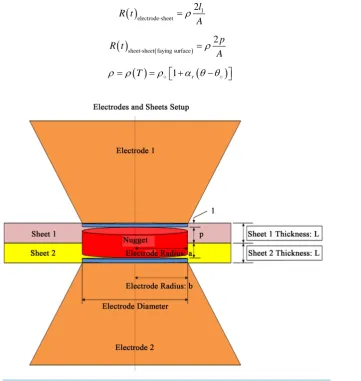
To start with, we consider a simplified heat balance model of a RSW process, presented in [13]. The simplified dynamical model of a RSW process determines the heat balance in the system as a function of nugget tempera-ture. For a simplified nugget model, shown in Figure 2, the heat balance can be described by the following equ-ations:

The total heat generation rate, Qg

( )

t is given by

( )

2

( ) ( )

g

Q t =I t R t (1a)

( )

w c e

R t =R +R +R (1b)

where I t

( )

denotes the welding current, and R t

( )

denotes the total resistance consisting of the resistance of work pieces, Rw, contact resistance, Rc, and electrode resistance, Re. Since Rw and Re are very small compared to the total contact resistance Rc, Rw and Re can be neglected in (1b).

The total contact resistance can then be described as,

( )

electrode-sheet

( )

sheet-sheet faying surface_{( )} c

R =R t +R t (1c)

A linear relationship between the resistance and temperature is assumed to model the heat generated as a function of temperature. Thus,

( )

1

electrode-sheet 2l R t

A ρ

= (1d)

( )

sheet-sheet faying surface_{( )} 2p R t

A ρ

= (1e)

( )

T 1 _r

(

)

[image:3.595.134.496.328.710.2]

ρ ρ= =ρ__ +α θ θ− _ _ (1f)

where ρ denotes the resistivity of the material, l1 denotes the distance from the melting interface to electrode contact surface, p denotes the penetration, A is the cross sectional area, ρ_ denotes the resistivity at reference temperature θ_, θ and αr are the temperature to be controlled and the temperature coefficient respectively.

Substituting (1f) in (1d) and (1e) we get

( )

electrode-sheet 1

( )

2

R t =cθ t +c (1g)

( )

sheet-sheet faying surface_{( )} 3

( )

4

R t =cθ t +c (1h)

where 1 1 2l c A ρ α_°

= (1i)

(

)

1 2 2 1 r l c A

ρ° _{α θ}

°

= − (1j)

3 2p c

A ρ α_°

= (1k)

(

)

4 2 1 r p c A

ρ_{° α θ}

°

= − (1l)

Substituting (1g) and (1h) in (1a) we get

( )

2

( )

(

( )

( )

)

1 2 3 4

g

Q t =I t cθ t + +c cθ t +c (1m)

( ) ( )

( )

2 2

5 6

c I t θ t c I t

= + (1n)

where

5 1 3

c = +c c (1o)

6 2 4

c =c +c (1p)

The heat of fusion required for nugget formation is given by:

f n

H = ∆H V (2a)

2 π

n

V a p

∆ = (2b)

where H denotes the heat of fusion per unit volume, ∆Vn denotes the nugget volume, and p, a denote the pene-tration and nugget radius respectively. Substituting (2b) in (2a) and normalizing over the weld duration, ∆t, we get the heat of fusion per unit time:

2 7 π

f

H

H a p c

t = =

∆ (2c)

Neglecting the heat loss in the surroundings and the electrodes, the heat required to raise temperature by

( )

dθ t is given by

( )

( )

dQ_T t =ρC_pdθ t ∆V (3a)

where ρ denotes the density, Cp denotes the specific heat, V is the volume, and dθ

( )

t is the tempera-ture rise. We rewrite (3a) as:

( )

8

( )

where

2 8 pπ c =ρC a p

(3c)

The total heat loss rate is given by

( )

( )

( )

L a r

Q t =Q t +Q t (4a)

( )

1

( )

2 1

1

10

π t t L

k a

l b

θ θ θ β

α −   = _ + _  

( )

2 2 2

1 1 1 1

1 1

π 10 π π

k a k a L k a

t

l b l

β _θ θ

α   =_ + _ −  

( )

9 10

cθ t c

= − (4b)

where

2 2

1 1

9 1

π 10 π

k a k a L

c l b β α   =_ + _

  (4c)

2 1 1 10 1 π k a c l θ = (4d)

In the above equations, Qa

( )

t and Q tr

( )

denote the axial and radial loss rates, respectively; k1 repre-

sents thermal conductivity, a is the nugget radius; θ

( )

t , θ1, represent the melting temperature and the inter-face temperature at the work piece respectively; l1 is the distance from the melting interface to the electrodes contact area; β represents the final penetration to work piece thickness ratio; L is the sheet thickness; ,bα represent the electrode radius and thermal diffusivity of work piece respectively.

The heat balance equation over time

(

t t, +dt

)

is given by

( )

f d d

( )

( )

d

g T L

H

Q t t Q t Q t t

t

= + +

∆

  ₍₅₎

Substituting (1n), (2c), (3b), and (4b) in (5) and rearranging it, we get

( )

2

_{( ) ( )}

2

_{( )}

_{( )}

8 5 6 9 10 7

d

d t

c c I t t c I t c t c c

t θ

θ θ

= + − + − (6a)

or, equivalently,

( )

2

_{( ) ( )}

2

_{( )}

_{( )}

11 12 13 14

d d

t

c I t t c I t c t c

t θ

θ θ

= + − + (6b)

where

11 5 8

c =c c (6c)

12 6 8

c =c c (6b)

13 9 8

c =c c (6c)

(

)

14 10 7 8

For the sake of notational convenience, let y t

( )

=θ

( )

t and _{u t}

( )

=_I2

( )

_t

. Then (6b) can rewritten as

( )

_{( ) ( )}

_{( )}

_{( )}

11 12 13 14

d

d y t

c u t y t c u t c y t c

t = + − + (7)

Equation (7) represents a bilinear electrothermal dynamical model of a RSW process. Note that this simplified model neglects the heat required to raise the temperature of the electrodes and the nugget surroundings. Also, it assumes that most of the heating occurs near the faying surface due to its high contact resistance. The size of the workpieces is assumed to be infinite in the radial direction and the nugget shape is assumed to be a disk growing radially and axially in the same proportions. The nominal nugget diameter is assumed to be 4.5 L, where L is the sheet thickness.

Using a first order Euler approximation for d d y

t with a sampling period Ts, the following discrete time equ-ation is derived from the system Equequ-ation (7):

(

) ( )

_{( ) ( )}

_{( )}

_{( )}

11 12 13 14

1

s

y k y k

c u k y k c u k c y k c

T + −

= + − + (8a)

or

(

1

)

( )

( )

( ) ( )

y k+ =Ay k +Bu k +Cu k y k +D (8b)

where

13

1 _s

A= −c T (8c)

12 s

B=c T (8d)

11 s

C=c T (8e)

14 s

D=c T (8f)

Also, k denotes the discrete time index

(

k=0,1, 2,

)

and kTs denote the sampling instances. The above electrothermal model is characterized by four unknown parameters, namely, A, B, C, and D.

3. Design of a RSW Controller

To develop a control scheme for controlling the nugget temperature of the RSW model presented by Equation (8a), we realize that it presents a bilinear system characterized by some unknown parameters. These parameters can vary from weld to weld, and in most cases we have no prior knowledge of the parameter values. In view of this, we propose to use an adaptive OSA and WOSA controllers.

The proposed adaptive control scheme involves measurement of the inputs and outputs of the system, estima-tion of unknown system parameters using a recursive least squares (RLS) parameter estimaestima-tion algorithm, and computation of a control signal based on the estimated parameter values. Also, the temperature of the weld nugget is monitored indirectly by assuming it to be proportional to the contact resistance.

3.1. Adaptive OSA and WOSA Controllers

In an adaptive controller, the sampled measurements, u k

( )

and y k

( )

, are used to estimate the model para-meters, A B C, , and D in Equation (8b), using a recursive parameter estimation method, such as recursive least square (RLS). The estimated values of these parameters are then used to compute the OSA/WOSA control sig-nals.

3.2. Parameter Estimation

First we write model Equation (7) in the following form:

(

₁

)

( )

T *

where

( )

T

(

) (

) (

) (

)

T

1 1 1 1 1

k y k u k y k u k

ϕ =_ − − − ∗ − _ (9b)

[

]

T

*

X = A B C D (9c)

Next, the estimated value of θ° is computed recursively using the following RLS algorithm:

( )

(

)

(

) (

)

(

) (

) (

)

( ) (

) (

)

T T

2 1

ˆ ˆ _{1 1} ˆ _{1 ; 1}

1 1 2 1

P k k

k k y k k k k

k P k k

ϕ

θ θ ϕ θ

ϕ κ

− − _{ }

= − + _ − − − _ ≥

+ − − − (10a)

(

)

(

)

(

) (

) (

) (

)

(

) (

) (

)

T T

2 1 1 2

1 2

1 1 2 1

P k k k P k

P k P k

k P k k

ϕ ϕ

ϕ ϕ

− − − −

− = − −

+ − − − (10b)

( )

[

]

T

ˆ 0 0 0 0

X = γ (10c)

( )

1

P − =σI (10d)

where γ >0 is a small number and σ >0 is chosen to be large. Also, C kˆ

( )

is always constrained to be non-negative, i.e.,

( )

ˆ _{0 for all}

C k > >ε k (10e)

Given an estimate X kˆ

( )

of *

X , we define the predicted output at time k+1 as:

(

)

( )

T _ˆ

( )

ˆ 1

y k+ =ϕ k X k (11)

3.3. Adaptive-One-Step-Ahead Tracking Controller

One-step-ahead (OSA) control scheme for linear systems has been well investigated in [14]. An OSA controller attempts to bring the predicted output, y k

(

+1

)

at time k+1, to the desired value, _y*

(

_k+1

)

in one step. Thus, it minimizes the following cost function:

(

)

(

)

_*

(

)

2

1

1

1 1 1

2

J k+ = _y k+ −y k+ _ (12)

The corresponding OSA control law is given by [14]:

( )

y*

(

k 1

)

Ay k

_{( )}

( )

D u k

B Cy k

+ − −

=

+ (13)

The above control signal needs to be constrained by the maximum current delivery capacity of the controller,

max

u , as follows:

( )

( )

( )

( )

( )

max max max

, if 0

0, if 0

, if )

u k u k u

u k u k

u u k u

< <   =_ ≤  _≥  (14)

The adaptive OSA controller uses the estimate, X kˆ

( )

in Equation (11) to compute the control signal, u k

( )

, from the following adaptive version of Equation (13) above:

( )

(

)

( ) ( )

( )

( )

( ) ( )

* _{ˆ ˆ}

1 ˆ ˆ

y k A k y k D k

u k

B k C k y k

+ − −

=

+ (15)

where A kˆ

( ) ( ) ( )

,B kˆ ,C kˆ , and D kˆ

( )

denote the estimated values of A B C, , , and D, respectively, at time

One of the potential drawbacks of OSA controllers is excessive control efforts that often result from attempt-ing to brattempt-ing y k

(

+1

)

to *

(

)

1

y k+ in one step. To address this potential problem, an AWOSA controller is discussed below.

3.4. Adaptive Weighted One-Step-Ahead Controller

The excessive effort to bring the output y k

(

+1

)

to the desired value _y*

(

_k+1

)

in one step using AOSA may result in an unfavorable saturation of the input. The adaptive weighted one-step-ahead controller attempts to seek a tradeoff between tracking accuracy and control effort by considering a slight generalization of the cost function (12) to the form (16) given below. Thus, it minimizes the following cost function:

(

)

(

)

*

(

)

2

( )

2

2

1

1 1 1

2 2

J k+ = _y k+ −y k+ _ +λu k (16)

where, 0< <λ 1 is chosen to provide a desired tradeoff.

The minimization of the cost function in (16) leads to the weighted one-step-ahead control law [14]:

( )

(

( )

)

(

(

)

( )

)

( )

(

)

2

1

B Cy k y k Ay k D

u k

B Cy k λ

+ + − −

=

+ + (17)

The above control law is also constrained by the maximum current delivery capacity, umax, as shown in Equa- tion (14) above. The choice of λ provides a desired tradeoff between tracking accuracy and control effort. A small λ results in good tracking but requires high level of control effort. A large λ, on the other hand, re-duces control efforts at the cost of tracking accuracy.

The adaptive WOSA controller uses the estimate, X kˆ

( )

, in Equation (11) to compute the control signal,

( )

u k from the following adaptive version of Equation (17) above:

( )

(

( )

( ) ( )

)

(

(

)

( ) ( )

( )

)

( )

( ) ( )

(

)

2

ˆ ˆ

ˆ ₁ ˆ

ˆ ˆ

B k C k y k y k A k y k D k

u k

B k C k y k λ

+ + − −

=

+ + (18)

where A kˆ

( ) ( ) ( )

,B kˆ ,C kˆ , and D kˆ

( )

denote the estimated values of A B C, , , and D, respectively, at time

. k

4. Simulation Results and Discussion

This section presents the results of a simulation study showing the performance of the system with the proposed AOSA and AWOSA controllers and also compare them with a PID controller. Each controller is designed for tracking a reference temperature profile.

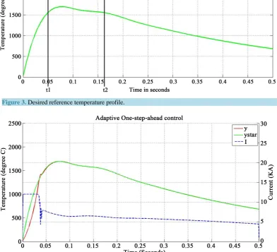
The reference temperature profile is a good indicator of the weld quality. Therefore, it is desirable to keep the temperature variation close to a desired variation curve, which may be experimentally predetermined for the good welds. A typical reference temperature profile for good weld is shown inFigure 3 below [1]. Basically, such a curve is characterized by a fast rise of temperature to melting point, melting of the workpieces at the fay-ing surface area which causes a slight drop in temperature, followed by a coolfay-ing zone that results from removal of weld current. The actual nugget temperature is measured during the weld cycle using the relationship de-scribed by Equation (1f). Depending on the tracking error signal, the welding current is adjusted so as to reduce the temperature error.

[image:9.595.102.492.279.459.2]

Figure 4 shows the performance of the AOSA controller using Imax =12 KA, where Imax denotes the maximum current delivery capacity of the weld controller. We can see that the AOSA controller adapts to the parameter change and force the output temperature profile to follow the desired temperature profile. Also, we can see that the energy required for the weld is lower than that of the PID controller.

Figure 5 and Figure 6 show the performance of AWOSA controller using Imax =12 KA with λ=0.1 and 1, respectively. Here we notice that when λ is high, the output temperature profile does not follow the desired output temperature profile well. However, increasing λ results in decreasing the total energy required for the weld.

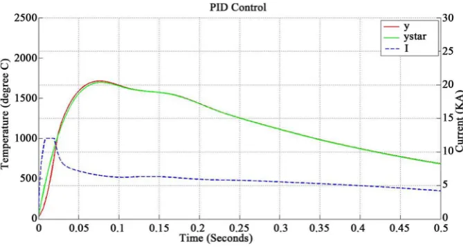
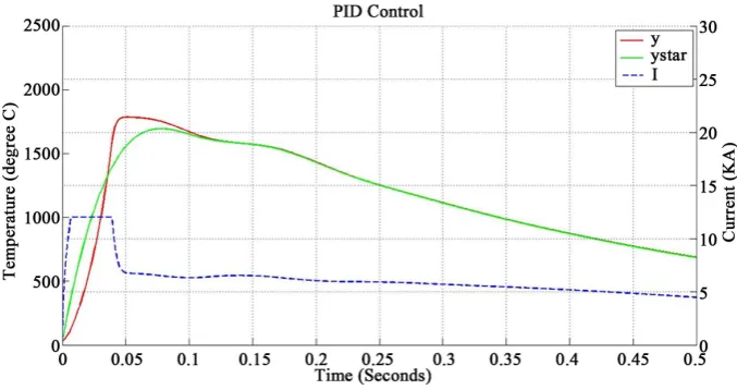
Figure 7 shows the performance of the PID controller prior to any parameter change using Imax =12 KA. After multiple trial and error attempts to get satisfactory results, the parameters of the PID controllers are: Pro-portional (P) = 0.5, Integral (I) = 26.56, Derivative (D) = 0.

In Figure 8we see that the PID controller looses track of the reference temperature profile due to weld para-meters change. Also, we can see that PID controller requires more energy for the weld comparing to AOSA and AWOSA.

[image:9.595.102.495.325.682.2]

Figure 3. Desired reference temperature profile.

[image:10.595.129.464.86.263.2] [image:10.595.135.462.305.470.2]

Figure 5. Performance of AWOSA Controller with 20% increase in nugget diameter and 50% increase in indentation; λ=0.1,I_max=12 KA, Energy=2558 W.

Figure 6. Performance of AWOSA Controller with 20% increase in nugget diameter and 50% increase in indentation; λ=1,Imax=12 KA, Energy=2470 W.

Figure 7. Performance of PID Controller prior to unknown parameter variations; Imax =

[image:10.595.130.465.513.692.2]

[image:11.595.128.467.85.264.2]

Figure 8. Performance of PID Controller with 20% increase in nugget diameter and 50% in-crease in indentation; I_max=12 KA, Energy=2632 W .

Comparing the simulation results for the three controllers, we can see that AOSA and AWOSA controllers compensate for the parameter variations and track the reference temperature profile quite well. Simulation re-sults in Figure 5for the AWOSA controller show satisfactory performance and a good tradeoff between track-ing error and total energy required for the weld regardless of change in weld parameters. The output temperature profile follows the desired temperature profile reasonably well during the heating stage prior to the melting point. Also, we can see that the total energy required to make a weld using AWOSA is reduced by 6% comparing to the PID controller when Imax =12 KA. This can result in significant energy savings for applications requiring a high volume of spot welds, such as manufacturing of automotive vehicles.

5. Conclusion

This paper presents a new approach for designing adaptive OSA and WOSA controllers for resistance spot welding processes by utilizing a simplified electrothermal dynamical model of the process. Simulation results of AOSA and AWOSA performance are compared with those of a PID controller. These results indicate that using the proposed AOSA and AWOSA controllers, the nugget temperature profile is forced to track a desired refer-ence temperature profile in presrefer-ence of unknown parameter variations. Also, these controllers reduce the energy consumed to perform a spot weld, which can result in significant energy savings for applications requiring a high volume of spot welds, such as manufacturing of automotive vehicles.

References

[1] Zhang, H. and Senkara, J. (2012) Resistance Welding Fundamentals and Applications. Taylor & Francis Group, Boca Raton.

[2] Govik, A. (2009) Modeling of the Resistance Spot Welding Process. M.S. Thesis, Institute of Technology, Linkopings University, Linkoping.

[3] Won, Y.J., Cho, H.S. and Lee, C.W. (1983) A Microprocessor-Based Control System for Resistance Spot Welding Process. Proceedings of ACC, San Francisco,22-24 June 1983, 734-738.

[4] Zhou, K. and Cai, L. (2014) A Nonlinear Current Control Method for Resistance Spot Welding. Proceedings of ASME Transactions on Mechatronics, 19, 559-569. http://dx.doi.org/10.1109/TMECH.2013.2251351

[5] Salem, M. and Brown, L.J. (2011) Improved Consistency of Resistance Spot Welding with Tip Voltage Control. Pro-ceedings of CCECE, Niagara Falls, 8-11 May 2011, 548-551. http://dx.doi.org/10.1109/ccece.2011.6030511

[6] Chen, X., Araki, K. and Mizuno, T. (1997) Modeling and Fuzzy Control of the Resistance Spot Welding Process. Pro-ceedings of SICE, Tokushima, 29-31 July 1997, 898-994.

[7] El-Banna, M., Filev, D. and Chinnam, R.B. (2006) Intelligent Constant Current Control for Resistance Spot Welding.

Proceedings of IEEE Conference on Fuzzy Systems, Vancouver, 16-21 July 2006, 1570-1577.

[8] Chen, X. and Araki, K. (1997) Fuzzy Adaptive Process Control of Resistance Spot Welding with a Current Reference Model. Proceedings of IEEE Conference on Intelligent Processing Systems, Beijing, 28-31 October 1997, 190-194. [9] Shriver, J., Peng, H. and Hu, S.J. (1999) Control of Resistance Spot Welding. Proceedings of ACC, San Diego, 2-4

June 1999, 187-191. http://dx.doi.org/10.1109/acc.1999.782766

[10] Ivezic, N., Allen Jr, J.D. and Zacharia, T. (1999) Neural Network-Based Resistance Spot Welding Control and Quality Prediction. Proceedings of IPMM, Honolulu, 10-15 July 1999, 989-994. http://dx.doi.org/10.1109/ipmm.1999.791516

[11] Messler Jr, R.W., Jou, M. and Li, C.J. (1995) An Intelligent Control System for Resistance Spot Welding Using a Neural Network and Fuzzy Logic. Proceeding of IAC, Orlando, October 1995, 1757-1763.

http://dx.doi.org/10.1109/ias.1995.530518

[12] Kim, E.W. and Eagar, T.W. (1988) Parametric Analysis of Resistance Spot Welding Lobe Curve. SAE Technical Pa-per Series, Warrendale.

[13] Kas, Z. and Das, M. (2014) A Thermal Dynamical Model Based Control of Resistance Spot Welding. Proceedings of IEEE EIT 2014, Milwaukee, 5-7 June 2014, 264-269. http://dx.doi.org/10.1109/eit.2014.6871774

Appendix

Boundedness of Nugget Temperature

Since a RSW is a time limited process (∆ <t 0.5 sec usually), establishing a proof of asymptotic tracking would be meaningless. However, it is important to make sure that the nugget temperature remains bounded during time

(

0,∆t

)

. A theoretical upper bound of the nugget temperature rise, ∆θ

( )

t , during time,

(

0,∆t

)

, can be estab-lished as follows.

Notice the amount of heat absorbed = the amount of heat supplied – the amount of heat loss Suppose

θ

∆ = rise in temperature during time,

(

0,∆t

)

Thus,

( )

Amount of heat obsorbed=CA∆θ t (19)

where CA is a constant.

( ) ( )

2 2

max max 0

Amount of heat supplied d

t

I t R t t tI R

∆

=

_∫

≤ ∆ (20a)

where

max r

R =R_°+ ∆α θ (20b)

and Imax denotes the maximum weld current.

Amount of heat lost=C_L∆θ (21)

where, CL is a constant. Thus,

(

)

2 max

A r L

C ∆ ≤ ∆θ tI R_°+ ∆ −α θ C ∆θ (22a)

or,

(

2

)

2

max max

A r L

C tI C tI R

θ α _°

∆ − ∆ + ≤ ∆ (22b)

or,

2 max 2 max

A r L

tI R

C tI C

θ

α° ∆ ∆ ≤

− ∆ + (22c)