A New No-reference Method for Color Image
Quality Assessment
Sonia Ouni
1,21
Team of research SIIVA, RIADI Laboratory
2
CReSTIC, University of Reims Champagne Ardenne Abou Raihane Bayrouni 2080,
Ariana, TUNISIA
Ezzeddine Zagrouba
Team of research SIIVA, RIADI Laboratory, University of Tunis El Manar, High Institute of ComputerScience (ISI)
Abou Raihane Bayrouni 2080, Ariana, TUNISIA
Majed Chambah
CReSTIC, University of ReimsChampagne Ardenne Rue des crayères BP 1035 51687
REIMS Cedex 2, FRANCE
ABSTRACT
Image quality assessment (IQA) is a complex problem due to subjective nature of human visual perception. Human have always seen the world in color. The widely objective metrics used are mean squared error (MSE), peak signal to noise ratio (PSNR), and human visual system based on structural similarity and edge based similarity. The problem of these objective metrics that they evaluate the quality of grayscale images only and don’t make use of image color information. Also, we must have the presence of original image. Unfortunately, the field of no-reference (NR) color IQA has been largely unexplored although the color is a powerful descriptor that often simplifies the object identification and extraction from a scene so color information also could influence human beings’ judgments. So, in this paper a new no reference methods for color IQA are proposed. These methods are based on different statistical analyses and easy to calculate and applicable to various image processing. This proposed metrics are mathematically defined and overcame the limitations of existing metrics to assess the quality of the color in the image. The experiment results on various image distortion show that our proposed no reference metrics have a comparable performance to the other traditional error summation metrics and to the leading metrics available in literature.
Keywords
Image Quality Assessment (IQA), No Reference (NR), color, objective metric, human visual perception.
1.
INTRODUCTION
In recent years, digital images and video data are subject to various kinds of distortions during acquisition, compression, processing, restoration, transmission, and reproduction. Measurement of image quality is fundamental importance to numerous grayscale image processing applications. So, in the last three decades, there has been rapid and enormous transition from grayscale image to colors ones [1]. The color plays a crucial role in many applications like print, photographs, television, restoration, cinema movies, database indexing and retrieval. Despite the importance of color there has been widely utilized and exploited for its properties in applications. But unfortunately, these images are subjected to wide variety of defects during its acquisition, subsequent compression, transmission, processing and then reproduction, which degrade visual quality. So, measurement of image quality is crucial for many image processing systems. The task of image quality assessment can be divided on two ways: subjective and objective [2].
Subjective methods for digital image (video) quality assessment are defined in ITU-R Rec. BT.500-11 [3]. They can be subdivided in three methods: Double Stimulus Impairment Scale Method (DSIS or EBU), Double-Stimulus Continuous-Quality Scale Method (DSCQS), Single-Stimulus and Stimulus-Comparison methods. In DSIS method, both reference and distorted set are shown to the assessor, which is expected to vote on the distorted set, while "keeping in mind the reference".
In Single Stimulus scaling, assessment is done on the image individually without any reference. In stimulus comparison scaling, assessment is done by comparing different distortions against each other. In DSIS method, single-stimulus and stimulus comparison methods, assessor is expected to grade using a list of possible values described verbally (imperceptible, perceptible but not annoying, slightly annoying, annoying, very annoying). In DSCQS method grading is on a continuous scale.
The basic idea of subjective methods is that a group of assessors (or even a single assessor) judges the quality of an image or video being presented to them. The overall difference in quality is given as the mean opinion score (MOS) which is computed as the mean value of the differences from all observers. Subjective methods are the most accurate in determining “how much” of image distortion can be perceived, and thus can measure the performance of objective assessment methods. The subjective methods are expensive and impossible to be included in automatic systems.
Instead, an objective image or video quality metric can provide a quality value for a given image or video automatically in a relatively short time. This is very important for real time applications. Objective metrics have, therefore, attracted more attention during recent years [4]. This approach can be classified into three categories: Full-reference (FR), Reduced-reference (RR) and No-reference (NR). Full-reference image quality assessment (FR-IQA) is based on measurement of differences between the original image or video and the distorted one. FR-IQA metrics have been intensively studied in literature.
assessment (NR-IQA), which looks only at the image or video under test, has no need for reference information. It is complicated in such application (digital photography, printing,…) where a reference is not available to measure the quality. Since the Human Visual System (HVS) never requires a reference to define the quality of an image it perceives, the principal problem is how to assess the image quality without no-reference. This way presents a new research direction, with promising applications but little progress [4] [5]. This paper presents a no reference image quality assessment method for color images where original test image is not available.
The objective image quality assessment metrics can be classified into two categories. The first is based on mathematical measures like Mean Squared Error (MSE), Mean Absolute Error (MAE), Root Mean Square Error (RMSE), Mean Absolute Error (MAE), Signal to Noise Ratio (SNR), Peak Signal-to-Noise Ratio (PSNR) and Spatial Color Image Quality Metric (SCID) [6]. The second is based on characteristics of the Human Visual System (HVS) like mean structural similarity index (MSSIM) [7]. Visual information fidelity in pixel domain (VIFP), structure and hue similarity (SHSIM) [8]. Also, most of these objective measures evaluate the quality of grayscale images only and don’t make use of image color information and they are FR-IQA. However, it is not always possible to get the reference images to assess image quality. Human observers can easily recognize the distortion and degradation of image without referring to the original image. Therefore, there is absolutely necessary to develop objective color quality assessment image.
In this paper, a new NR-IQA color is developed which overcomes the limitation of existing methods and takes in to account of the distribution of the chrominance in image. Parameters are selected based on the fact that they must be sensitive to distortions. The rest of the paper is organized as follows: Section II describes different existing methods of IQA and discusses the related work showing the reason why objective image quality assessment is important and necessary. In section III, presents highlights color image fundamentals. Section IV discusses the formulation of the proposed No Reference which is based on color followed by section V showing implementation and analysis of results. Finally, section VI draws conclusions and provides future works.
2.
IMAGE QUALITY ASSESSMENT
In this paper, we examined several commonly most widely used objective quality measures which give better correlation results with subjective [9]. There are as follows:
1. MSE 2. PSNR
3. Mean Structural Similarity Index MSSIM 4. Universal Image quality Index UQI 5. Visual information fidelity VIF
2.1
MSE & PSNR
The simplest and the most used metric is the mean squared error (MSE) which represents the power of noise or the difference between original and tested images.
N M j i b j i aMSE i j
. ,
, 2
(1)
where a(i,j) and b(i,j) are corresponding pixels from the original and tested images, and M and N describe height and width of an image.
Peak Signal Noise Ratio (PSNR) is also widely used although there is very well matched to human judgment of image. It represents the ratio between the maximum possible power of a signal and the power of noise. PSNR is usually expressed in terms of the logarithmic decibel, is given by:
MSE
PSNR10log10 255 (2)
where 255 is maximum possible amplitude for an 8-bit image.
2.2
Mean Structural Similarity Index
The Structural Similarity (SSIM) quality metric is built on the hypothesis that the human visual system is adapted to extract structural information from the scene [10]. Structural information can be defined as “the attributes that represent the structure of objects in the scene, independent of the average luminance and contrast” [11]. Thus, the perceived image distortion can be approximated by the structural information change detected between the reference and the test image. The similarity measure compares the original and the distorted signal considering three main features of images: the luminance, the contrast and the structure.Let X={xi|i=1,2,..,.N} and Y={yi|i=1,2,..,.N} be the original and test image respectively. The SSIM is given by this equation: [ ( , )] [ ( , )] )] , ( [ ) ,
(x y lx y cx y sx y
SSIM
(3)
Where α, β, and γ are parameters to define the relative importance of the three components l(x,y) is luminance comparison (eq. 4), c(x,y) is contrast comparison (eq. 5), and s(x,y) is structural comparison (eq. 6).
1 2 2 1 2 ) , ( C C y x l y x y x
(4) 2 2 2 2 2 ) , ( C C y x c y x y x
(5) 3 3 ) , ( C C y x s y x xy
(6) 3 2 1,C ,C
C are constants. x, y, x, y, xy are defined as
following:
1 1 1 1 , 1 1 , 1 , 1 1 1 2 2 1 2 2
N i y i x i xy N i y i y N i x i x N i i y N i i x y x N y N x N y N x N (7)
They applied the SSIM indexing algorithm for image quality assessment using a sliding window approach. The window moves pixel-by-pixel across the whole image space. At each step, the SSIM index is calculated within the local window. If one of the image being compared is considered to have perfect quality, then the resulting SSIM index map can be viewed as the quality map of the other (distorted) image. Instead of using a 8 × 8 square window is used for local statistics to avoid “blocking artifacts”. Finally, a mean SSIM (MSSIM) index of the quality map is used to evaluate the overall image quality and is defined as:
M
j SSIMxj yj
M Y X MSSIM 1 , 1 ) ,
(
(8)
2.3
Universal Image quality Index (UQI)
Instead of using traditional error summation methods, the method proposed by Wang and Bovik was designed to model any image distortion via a combination of three factors: loss of correlation, luminance distortion, and contrast distortion [12].Let X={xi|i=1,2,..,.N} and Y={yi|i=1,2,..,.N} be the original and test image respectively. μx is the mean of x, σx is variance of x, σy is variance of y and σxy is the covariance of x, y (eq. 7). So the Universal Quality Index UQI is defined as followed:
2 2 2 2 4 y x y x y x xy UIQ
(9)
This equation can be divided on three components and can be written as:
2 2
2 2
2 2 2 2 y x xy y x y x y x xy UIQ
(10)
The first component is the correlation coefficient between x and y, which measures the degree of linear correlation between and x and y. The second component measures how close the mean luminance is between x and y. The third component measures how similar the contrasts of the images are as σx and σy can be viewed as estimate of the contrast of x and y.
UIQ = correlation • (luminance) • contrast
2.4
Visual Information Fidelity in Pixel
Domain (VIFP)
The visual information fidelity in pixel domain (VIFP) measures the mutual information between the input and the output of the HVS channel for both the original and distorted images. Assumption was made that, in the absence of any distortions, this signal passes through the HVS channel of a human observer before entering the brain, which extracts cognitive information from it. For distorted images, it was assumed that the reference signal has passed through another distortion channel before entering the HVS. Combining these two quantities, a visual information fidelity measure for IQA is derived. But, for distortion types that are significantly different from blur and white noise, such as JPEG compression, the model fails to reproduce the perceptual annoyance adequately and also to implement VIFP criterion in, a number of assumptions are needed about the source, distortion, and HVS models.
3.
COLOR IMAGE QUALITY
A color image can be represented in different color space for different applications. In color image processing, there are various color models in use today. The RGB model is mostly used in hardware oriented application such as color monitor. In the RGB model, images are represented by three components, one for each primary color : red, green and blue. Although human eye is strongly perceptive to red, green, and blue, the RGB representation is not well suited for describing color image from human perception point of view. Moreover, a color is not simply formed by these three primary colors. When viewing a color object, human visual system characterizes it by its brightness and chromaticity. The latter is defined by hue and saturation. Brightness is a subjective measure of luminous intensity. It embodies the achromatic notion of intensity. Hue is a color attribute and represents a
dominant color. Saturation is an expression of the relative purity or the degree to which a pure color is diluted by white light. The HSV model is motivated by the human visual system. In the HSV model, the luminous component (brightness) is decoupled from color-carrying information (hue and saturation). The HSV color model is defined as follows [13]: MAX V if MAX if MAX MAX S if MAX defined not B if MAX B G G if MAX B G R if MAX B G H 0 0 0 0 4 60 2 60 60
(11)
where δ=(MAX-MIN), MAX=max(R,G,B) and MIN=min(R,G,B). It is more natural for human visual system to describe a color image by the HSV model than by the RGB model.
[image:3.595.330.525.485.678.2]Intuitively, the features extracted in the HSV color space can capture the distinct characteristics of computer graphics better. For example, computer graphics is more color smooth than photographic images in the texture area. Fewer colors are contained in computer graphics. Intensity of computer graphics reveals different characteristic of edge and shade. These differences between computer graphics and photographic images are best described by decoupling the intensity from chromatic information, say, hue and saturation. Inspired by the way human visual system perceives the color object, we propose to construct a metrics from the HSV color space. For the purpose performance color metrics, in the next section, we will base on HSV color model.
4.
PROPOSED COLOR IMAGE
QUALITY
4.1
Hue Polar Histogram
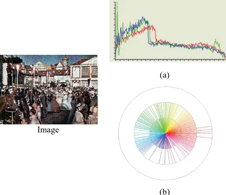
The most important evaluation is related to color cast and chromatic diversity. Our evaluation is based on the proposed hue polar histogram (HPH). It represents a hue circle of all the hues present in the image. Each hue is represented by a spoke (radius) joining the centre to the hue value. The histogram is made easier to read by plotting each spoke with the color it represents. Hence the HPH summarizes the chromatic diversity of the image.
The length of the spokes is proportional to the size of the population having the same hue. It shows the predominant hues of the image. Figure 2 illustrates in the first the histograms of image and in the second the usefulness of the HPH in evaluating the predominant color and the chromatic diversity of the image.
Image
(a)
(b)
Fig 2: (a) histograms, (b) Hue Polar Histogram.
4.2
Dispersion of the dominant color in the
image:
To determine the quality of the image color, we will be interested in the presence of the image dominant color. We propose a no reference measure named: Dispersion of the dominant color and noted: . It is based on the circular statistical and directions that can analyze data [14] (example the hue). Von Mises distribution is the most frequently used in the analysis of direction and in circular statistics, it plays a role similar to the usual normal distribution N (,2). The (concentration) is very similar to the variance , it can be interpreted by a low variance of thus a high value of variance. The following equation defines the parameter of the set {Xi}i=1,n :
i i
i i i
i x x
x n
A1 1 cos with : arctan sin , cos
1
(12)
The parameter is the means and the function arctan gives the angle between the axis X and the vector. The function
1 1
A is the inverse function of the first order Bessel function. This approach is very reliable for the detection and
identification of a dominant color. Fig. 2 presents two images and their hue polar histogram.
The first one presents a chromatic diversity but the second one shows a bleu dominant color which is illustrated by their hue polar histogram.
(a) μ= 123(deg), κ= 18.33614
(b)
[image:4.595.330.547.140.351.2]μ= 231(deg), κ = 114.972
Fig 3: Example of the dominant color dispersion.
This metric can detect the presence of a dominant color having hue equal μ. Having a large value of κ or a high concentration indicates a dominating color that is illustrated in figure 3. Therefore, in figure 4, the polar histogram image presents a concentration explained by the high value of k but in this case, the dominant color is natural and it is not an artifact. Thus, in this case, this metric can not distinguish the difference between natural and artifact color dominant.
[image:4.595.55.287.280.481.2]μ = 177, k = 87.27745, Π = 0.8381
Fig 4: Example of the dominant color dispersion.
To resolve this problem, we propose to define a new no reference color assessment metric named: Spatial Distribution of the dominant color. It permits to indicate if the dominant color is an artifact when the color is propagate in all image or if there is a natural dominant (such as sea, sky…).
4.3
Portion of the dominant color:
Π
The portion Π represents the percentage of pixels belonging to the dominant color and it is defined as follows:
N M NPDC I
[image:4.595.330.517.470.562.2]where M× N represents the size of image I. NPDC is a set of pixels which belongs to the dominant color.
xi j i N j M colorxi j c
NPDC , , =1... , =1... / , (14)
4.4
Spatial distribution of the dominant
color:
DS
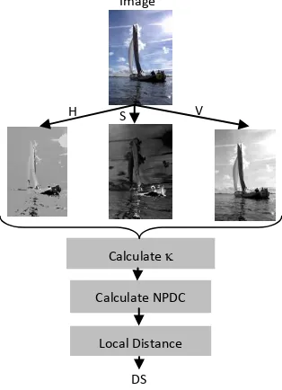
[image:5.595.81.238.216.433.2]The statically metrics and Π are not sufficient for evaluating color image so we define a new criterion named Spatial Distribution of the dominant color and noted DS. The figure 5 presents the different steps.
Fig 5: Different steps of Spatial Distribution.
The criterion defines a measure of the spatial dispersion of the dominant color in the image. Let NPDC is the set of pixels which belongs to the dominant color. The distance between every pixel Pi and all the pixels of this set is the local distance (LD) calculates as follow:
P NPDCNPDC card
P P d P
P
LD i
NPDC
j j i
j
i
,
,
, 1 (15)
where:d
Pi,Pj
xPixPj
2 yPiyPj
2 (16)Subsequently, the spatial dispersion of the dominant color in the image I is as follows:
NPDC card
LD I
DS
NPDC
i i
1 (17)
The examples in Figure 8 show the importance of this metric to give information about the spatial dispersion of the dominant color.
Fig 6: Example of spatial distribution.
In fig 6 (a) and (b), we observe that the two images have the same portion of a dominant color Π1= Π2=0.69 but this is not sufficient to define whether there is a dominant color situated in the part or in the whole image. Therefore, the dominant which is situated in a partial part of the image generally presents a natural image. For example, the dominant color represents the color of an object; however, if the dominant color is situated in the whole image, it will then indicate that it is not a chromatic diversity. As a result, we are having a fading color and a bad quality. The metric of Spatial Distribution permits to give this information in Fig 6(a) and (b) although we have the same proportion of the dominant color but we have not the same value of spatial distribution.
The first one presents a dominant color concentrated in the part of the image but the second is propagates in the whole image. When the DS is increasing, this explains that the dominant is situated in all parts of the image which is the case in Fig 6 (b).
5.
EXPERIMENTAL RESULTS &
DISCUSSION
In order to evaluate the performance of proposed quality metrics we propose a new image database. Although, the largest database of distorted test images has been created, they are dedicated to specific domain applications like compression or transmission. The LIVE image database [15] is composed of 982 distorted images: 29 color reference images and their distorted images using the following distortion type: JPEG2000, JPEG, White noise, Gaussian blur, and bit errors, 5-7 distortion levels. Every distorted image includes corresponding Difference Mean Opinion Score (DMOS). However, the LIVE database as well as the other ones, do not allow to adequately evaluating metrics of image visual quality [15]. This is due to the limited number of the modeled types of distortions, for example in LIVE, we find JPEG and JPEG2000 compression, arising from transmission errors for JPEG2000, modeled by white noise and Gaussian blur.
Among them, only the distortion caused by JPEG compression allows the evaluation of the correspondence of the tested metrics to one feature of HVS. Therefore, [16] defines the TID2008 database which contains 25 reference images and 1700 distorted images (25 reference images x 17
(a) Π1 = 0.69 DS= 0.0098
(b)
Π2 = 0.69 DS =0.0020936
S Image
Calculate
Calculate NPDC
Local Distance
H V
types of distortions x 4 levels of distortions). All of these distortions are detailed in [17] [16]. The LIVE and the TID2008 databases present some types of distortions especially induced by JPEG and JPEG2000. In our case, we interested in evaluating the color of quality image which is based on many artifact for example the effect of dye bleaching is seen as an overall color cast and a loss of contrast, saturation and chromatic diversity. This artifact is due of the presence of illuminant like in fig.7 (a) or old photographic images fig 7(b).
[image:6.595.313.544.85.243.2]
(a) (b)
Fig 7 : Example of the effect of dye bleaching.
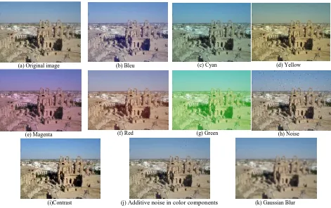
[image:6.595.58.276.186.291.2]For this reason, we propose a test database that contains color images with different textural characteristics, various percentages of homogeneous regions, edges and details. This database is composed of 15 reference images of varied themes altered with 10 types of degradation for each one (fig.8). The distortions are shown in the table 1. For every type of distortion, there are 6 different levels. Images are judged by 15 observers with the protocol SSCQS to rate the overall quality of the image.
Table 1. Different distortions used N Type of distortion
(six levels for each distortion)
Correspondence to practical situation
1 Dominant color Red Image acquisition 2 Dominant color Green Image acquisition 3 Dominant color Bleu Image acquisition 4 Dominant color cyan Image acquisition 5 Dominant color magenta Image acquisition 6 Dominant color Yellow Image acquisition 7 Additive noise in color
components
Image acquisition
8 Contrast Image acquisition
9 Impulse noise Image acquisition 10 Gaussian Blur Image registration The proposed color metrics is no reference it can be applied for any image without the necessity of the presence of the original one but in the literature the most used metrics are full reference to assess the quality.
For this reason to prove the performance of the proposed metrics we will compare it to different quality full reference measures like MSE, PSNR [18], MSSIM [19], UQI, VIFP. Quality will also be evaluated for different levels of distortions for each quality metric. However, performance of proposed metrics and other existing metrics will also be checked at all level of distortions i.e. level 1 (minimum distortion), level 2, level 3, level 4, level 5, level 6 (maximum distortion).
(a) Original image (b) Bleu (c) Cyan (d) Yellow
(e) Magenta (f) Red (g) Green (h) Noise
(i)Contrast (j) Additive noise in color components (k) Gaussian Blur
[image:6.595.71.542.403.699.2]The original image is compared with distorted one for the full reference. In case of original image 3(a) values of these metrics is maximum i.e. unity since it is completely undistorted image. MSE will be zero and PSNR will be infinite. For our proposed metric Dispersion of the dominant color () is no reference, so when we applied to original image we note that the value of k is the minimum. This means that there is a chromatic diversity in image. From table 2 it is HVS since PSNR qualityvalues are almost the same across
clear that, MSE & PSNR results are fully inconsistent with various distortion types although they are having different visual perception. Where, MSE values must increase in different distortions from example 3(b) to 3(i) according to HVS. But MSE results are completely inconsistent only in impulse noise image 3(h). Figure 9 and table 2 shows that proposed metric working accurately to prove the quality assessment of every distorted image especially for the distortion of color component.
Fig.
No Type of distortion
Quality Metrics
No-Reference Full - Reference
K Π DS UQI VIFP MSSIM PSNR MSE
3(a) Original Image 0.3205 0.0325 0.0339 1 1 1 Infinite 0
3(b) Dominant color Bleu 2.0107 0.9282 0.0015 0.9945 1 1 44.54 0.0839
3(c) Dominant color cyan 2.0208 0.9682 0.0014 0.9932 0.9838 0.9999 43.44 0.0823
3(d) Dominant color Yellow 1.3560 0.2156 0.0048 0.9932 0.9838 0.9999 43.66 0.0923
3(e) Dominant color magenta 2.1078 0.9559 0.0014 0.8380 0.9796 0.9994 43.07 0.0950
3(f) Dominant color Red 1.5022 0.2286 0.0058 0.9745 1.0558 0.9998 43.43 0.09103
3(g) Dominant color Green 2.3196 0.9982 0.0014 0.9078 0.9987 0.9996 44.34 0.0825
3(h) Impulse noise 1.6013 0.2482 0.0068 0.0151 0.0352 0.9933 29.17 0.5534
3(i) Contrast 0.7502 0.03603 0.0021 0.5547 1.0320 0.9991 40.13 0.1551
3(j) Additive noise in color
components 2.1018 0.9459 0.0014 0.8380 0.9796 0.9994 43.07 0.0950
3(k) Gaussian Blur 0.5876 0.6197 0.0048 0.7046 0.3858 0.9998 48.73 0.0583
0.9999 43.66 0.0923
3(e) Dominant color magenta 2.1078 0.9559 0.0014 0.8380
0,9796 0.9994 43.07 0.0950 3(f) Dominant color Red 1.5022 0.2286 0.0058 0.9745
1,0558 0.9998 43.43 0.09103 3(g) Dominant color Green 2.3196 0.9982 0.0014 0.9078
0,9987 0.9996 44.34 0.0825 3(h) Impulse noise 1.6013 0.2482 0.0068 0.0151
0,0352 0.9933 29.17 0.5534
3(i) Contrast 0.7502 0.03603 0.0021 0.5547
1,032 0.9991 40.13 0.1551 3(j) Additive noise in color
components 2.1018 0.9459 0.0014 0.8380 0,9796 0.9994 43.07 0.0950
3(k) Gaussian Blur 0.5876 0.6197 0.0048 0.7046
0,3858 0.9998 48.73 0.0583
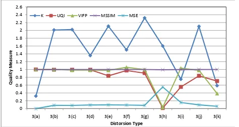
Table 2. Comparative quality measurement of image with different types of distortions at level 6.
0 0.2 0.4 0.6 0.8 1 1.2 1.4 1.6 1.8 2 2.2 2.4 2.6
3(a) 3(b) 3(c) 3(d) 3(e) 3(f) 3(g) 3(h) 3(i) 3(j) 3(k)
Qu
al
ity M
e
asu
re
Distorsion Type
[image:7.595.66.561.94.367.2]K UQI VIFP MSSIM MSE
[image:7.595.62.536.480.733.2]But UQI results are not consistent with HVS since the quality sequence is not followed by it.UQI is showing color distortion image 3(b) until 3(g) to be of higher quality which is not accordance to HVS. However, UQI show a less value of quality in additional noise 3(h) contrasted image 3(i) and blur image 3 (k) which is totally in consistent with HVS.
Also, results of visual information fidelity (VIFP) are completely violating HVS in case of distortion color, but very less value of quality even noise 3(h) contrast 3(i) and blur 3 (k). Similarly, the results of MSSIM are completely violating HVS in case of color image distortions 3(b) and 3(h) showing, maximum value of quality. Also MSSIM values are not following HVS based sequence of quality across other distortions. Inconsistent values of MSSIM values are in all types of distortions. The performance of the proposed metric is out of the other ones especially to evaluate the quality of the color in image.
6.
CONCLUSION
The most objective metrics are not interest to assess the color in image which presents important information for the human perception. In this paper, we present a new color no reference color method to IQA.
Experiments performed, on standard color images for wide variety of distortions indicate that proposed new color image quality metric in spatial domain is overcoming the limitation of existing quality methods discussed in the paper.
It is concluded that, MSE and PSNR values are showing very poor correlation with HVS. MSSIM, VIFP and UQI values are also not showing full consistency with HVS across various distortions discussed. However, the new no reference metric values are following desired HVS sequence of quality across various distortions as well as showing the consistent results at different levels of distortions especially to define the dominant color.
Until now, there is no common approach to evaluate the quality of images in different distortions caused by various automated image processing application like image compression, communication, acquisition, display, restoration, enhancement, segmentation, detection, and classification of photographic images, medical images, geographic images, satellite images, and the astronomical images. But to achieve the best image quality evaluation for these specific applications, there is still a lot more work to do. Color image quality assessment can be further extended to video quality assessment.
7.
REFERENCES
[1] N. Thakur and S. Devi. "A new Method for Color Image Quality Assessment ". International Journal of Computer Applications 15(2):10–17, February 2011.
[2] S. Ouni, M. Herbin, E. Zagrouba. "Are existing procedures enough? Image and video quality assessment: review of subjective and objective metrics ". Image Quality and System Performance, SPIE/IS&T Electronic Imaging, Proc. SPIE 6808, 68080Q, California, USA, 28-30 January 2008.
[3] Rec. ITU-R BT.500-11. Methodology for the subjective assessment of the quality of television pictures. ITU-R, 1974-2002.
[4] Y. Tian, M. Zhu, L. Wang, Analysis and Design of No-Reference Image Quality Assessment, pp.349-352, 2008 International Conference on Multi Media and Information Technology, 2008.
[5] S. Ouni, E. Zagrouba, M. Chambah, M. Herbin. No-Reference Image Semantic Quality Approach Using Neural Network. IEEE International Symposium on Signal Processing and Information Technology (ISSPIT) pp.95-102,December 14-17, Bilbao – Spain, 2011. [6] S. Ouni, M. Chambah, M. Herbin, E. Zagrouba. SCID:
Full Reference Spatial Color Image Quality Metric, SPIE/IS&T Electronic Imaging, Proc. SPIE 7242, 72420U, California, USA, 28-30 January 2009.
[7] Z. Wang, A. C. Bovik, H. R. Sheikh, and E. P. Simoncelli. "Image quality assessment: From error measurement to structural similarity", IEEE Transaction on Image Processing, vol. 13, pp. 600-612, 2004. [8] Y. Shi, Y. Ding Z, R.hang, Jun Li. "Structure and Hue
Similarity for Color Image Quality Assessment". In Proceedings of International Conference on Electronic Computer Technology, pp. 329 – 33, 2009.
[9] E. Dumic, S. Grgic and M. Grgic, "New image-quality measure based on wavelets". J. Electron. Imaging 19, 011018, 2010.
[10] Z. Wang, A. C. Bovik, H. R. Sheikh, and E. P. Simoncelli, "Image quality assessment: From error visibility to structural similarity", IEEE Transactions on Image Processing, vol. 13, no. 4, pp. 600-612, April 2004.
[11]A. B. Watson, A. J. Ahumada.A standard model for foveal detection of spatial contrast. Journal of Vision, vol. 5, no. 9, pp. 717-740. 2005.
http://vision.arc.nasa.gov/dctune/
[12]Z. Wang and A. C. Bovik. "A universal image quality index", IEEE Signal Processing Letters, vol. 9, pp. 81-84, 2002.
[13]Wen Chen, Yun Q. Shi, Guorong Xuan, "Identifying Computer Graphics Using HSV Color Model and Statistical Moments of Characteristic Functions", 2007 IEEE International Conference on Multimedia and Expo (ICME 2007), Beijing, China, July2-5, 2007.
[14] S. Rao Jammalamadaka, A. Sengupta, Topics in Circular Statistics, World Scientific Publishing Company. 2001. [15]A. Bouzerdoum, A. Havstad and A. Beghdadi. Image
quality assessment using a neural network approach, Proc. Fourth IEEE Intern. Symposium on Signal Processing and Information Technology (ISSPIT-2004), pp. 330–333, Rome, Italy, 18-21 Dec. 2004.
[16]Ponomarenko N., Carli M., Lukin V., Egiazarian K., Astola J., Battisti F. Color Image Database for Evaluation of Image Quality Metrics, Proc. of Intern. Workshop on Multimedia Signal Processing, Australia, pp. 403-408, Oct. 2008.
http://www.ponomarenko.info/tid2008.htm
[17]H. R. Sheikh, Z. Wang, L. Cormack, and A. C. Bovik, LIVE Image Quality Assessment Database, Rel. 2, 2005. http://live.ece.utexas.edu/research/quality
[18]Z. Wang and A. C. Bovik. "Mean squared error: love it or leave it? - A new look at signal fidelity measures". IEEE Signal Processing Magazine, vol. 26, no. 1, pp. 98-117, Jan. 2009.
![Fig 1: Single Hexcone HSV Color Model [13].](https://thumb-us.123doks.com/thumbv2/123dok_us/8124304.795067/3.595.330.525.485.678/fig-single-hexcone-hsv-color-model.webp)