Do interest rates matter? credit demand in the Dhaka Slums

Munich Personal RePEc Archive

Do interest rates matter? credit demand

in the Dhaka Slums

Dehejia, Rajeev and Montgomery, Heather and Morduch,

Jonathan

Asian Development Bank Institute

September 2005

Online at

https://mpra.ub.uni-muenchen.de/33146/

ADB Institute Discussion Paper No. 37

Do Interest Rates Matter?

Credit Demand in the Dhaka Slums

Rajeev Dehejia

Heather Montgomery

Jonathan Morduch

September 2005

Abstract

If the demand for credit by the poor changes little when interest rates increase, lenders can raise fees to cost-covering levels without losing customers. This claim is at the core of sustainable microfinance strategies that aim to provide banking services to the poor while eschewing long-term subsidies, but, so far, there is little direct evidence of this. This paper uses data from SafeSave, a credit cooperative in the slums of Dhaka, Bangladesh, to examine how sensitive borrowers are to increases in the interest rate on loans. Using unanticipated between-branch variation in the interest rate we estimate interest elasticities of loan demand ranging from -0.73 to -1.04. Less wealthy

Do Interest Rates Matter? Credit Demand in the Dhaka Slums*

1. Introduction

The advent of microfinance lending in the last two decades has been hailed as a key development in the fight against poverty. The New York Times (1997) editorial page, for example, has promoted microfinance as “a much-needed revolution” and “the world’s hot idea for reducing poverty,” and the United Nations General Assembly recognized the trend by marking 2005 as the International Year of Microcredit. Microfinance involves new banking institutions that work in poor communities, aiming to achieve both financial viability and transformational social impacts. New credit contracts have led to

surprisingly high loan repayment rates (most established microlenders can claim repayment rates well above 95 percent), and economists have focused on the way that the contracts mitigate adverse selection and moral hazard, problems that undermined alternative attempts to lend to poor households without collateral (e.g., Stiglitz, 1990; Laffont and Rey, 2003; Rai and Sjöström, 2003).1

But high repayment rates are insufficient to drive a revolution. The key to the expansion of microfinance globally, it is argued, depends on the success of microfinance as a commercial phenomenon, free from subsidy (Drake and Rhyne, 2002; Robinson, 2001). The promise hinges as much (or more) on the ability to contain costs and to price loans at interest rates that are high enough to generate profits. Once profitability is in hand, microlenders can expand globally with minimal external support. The logic of this part of the microfinance revolution is built on the idea that poor households are willing and able to pay interest rates for loans that fully cover the costs of lenders. A corollary of this logic is that the poorest borrowers, who also tend to be the most expensive to serve, will pay the highest prices for capital.

Implicit in this argument is a key – and untested – assumption: that poor households of the kind that take advantage of microfinance are not very responsive to changes in interest rates. Specifically, it is argued that poor households primarily seek

access to credit, not necessarily “cheap” credit. When poor households are not very

sensitive to price changes, prices can be raised without fear of losing the core customer base and suffering from mission drift.2 When that is so, microfinance institutions can offer credit at a sufficiently high interest rate to cover their operating costs and at the same time not merely skim the cream by appealing only to the most eligible borrowers.

In this paper, we test this something-for-nothing view. We take advantage of an unexpected price increase imposed by a lender in the slums of Dhaka to examine the degree to which poor households reduce their borrowing when faced with a higher interest rate.

* _{We are very grateful for access to data from SafeSave, Dhaka. Stuart Rutherford, Mark Staehle, and the}

senior staff of SafeSave have been very generous with their time in answering questions about the data and product rules. Elvira Kurmanalieva provided expert research assistance in Tokyo, and Sarojini Hirshleifer helped with the industry-level microfinance data. We have benefited from comments from Jonathan Zinman, David Porteus, and seminar participants at Columbia. We take all responsibility for the analyses and any errors.

1 _{The July 2003}

Microbanking Bulletin provides the highest quality data available, covering 124 leading microlenders. Their average portfolio at risk greater than 30 days is 2.8 percent.

2 _{This argument has held greater force in Latin America and Africa, where microfinance interest rates have}

Other than Karlan and Zinman (2005), we know of no other econometric estimates of interest elasticities for customers in the microfinance market.3 The main methodological difficulty is that the schedule of interest rates seldom varies within a given program, and, when it does change, it does so for everyone across the board. Thus it is typically impossible to disentangle the effect of the interest rate change from broader changes occurring simultaneously (e.g., macroeconomic shocks). It may be possible to compare clients of different institutions who face different interest rates at any given moment, but then researchers face the question of why some customers selected one institution and why others selected another. It is also difficult to disentangle the effects of non-price differences among programs.

We use the administrative records of SafeSave, an innovative microfinance institution operating in the slums of Dhaka, to address this question. Identification is based on unanticipated between-branch variation in the interest rate. At the time of our study, SafeSave operated three urban branches, with slightly different products and prices in one of the branches. By comparing times at which product rules changed in two locations but not in the third, we can make inferences about the sensitivity of

customer behavior to interest rates. The SafeSave data allow a clean comparison based on an unexpected policy change made within a single institution that maintains a uniform philosophy and operating protocol throughout.

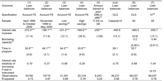
Our results suggest that borrowers are in fact highly sensitive to interest rate changes. After controlling for generally upward trends in loan demand, the implied elasticities of loan demand with respect to changes in the interest rate are in the range -0.73 to -0.88, with estimates as low as -1.04. We also find that less wealthy households (as measured by initial savings balances) are particularly sensitive to the interest rate increase (an elasticity of -0.86 compared to -0.26), and consequently that the bank’s portfolio shifted slightly away from its poorest borrowers when it increased the interest rate. The rate increase helped SafeSave to improve its financial condition, but not without a cost in terms of outreach to the poorest clients.

The paper is organized as follows. Section 2 reviews the prior literature and debates on interest rates. Section 3 provides details on SafeSave. Section 4

summarizes our data. Section 5 outlines our identification strategy. Section 6 presents results on the interest elasticity of loan demand. Section 7 concludes.

2. Interest Rate Debates

The assumption of inelastic demand for capital is a radical break from past thinking. In the 1970s and 1980s, usury laws were common, and they restricted interest rates on loans to low levels. These caps were often combined with directives on who should get subsidized loans and for what purpose.4 The laws were driven by the belief that high

3

Gross and Souleles (2002) provide estimates of the sensitivity of credit card customers in the United States to interest rate changes. Their findings are in the same range as ours. They find that the long-run (at the end of one year) elasticity of debt to the interest rate is -1.3, which is greater (in absolute value) than our estimates, but they find a smaller (in absolute value) elasticity for interest rate increases than decreases. Under half of their elasticity comes from shifting balances between accounts and the rest is from reduction in total debt. Karlan and Zinman (2005) provide interesting evidence that relates to the question here, finding that a one percentage point per month increase in the stated interest rate for loans (offered in a direct mail solicitation letter by a bank in South Africa) reduces the take-up of the solicitation by -0.3 percentage points (from an average take-up rate of 7 percent).

4 _{See, for example, the critical discussion in Adams, et al (1984). Homer and Sylla (1996) document how}

interest rates on working capital would consume most of the surpluses generated by small-scale entrepreneurs, leaving borrowers with little net gain. In Brazil in the early 1970s, for example, interest rates on loans for working capital were fixed at 17 percent per year while inflation rates ranged from 20 to 40 percent per year.5 _{Even where}

interest rate caps allowed positive real interest rates, they were seldom high enough to permit banks to cover costs. As a result, lending to the poor was a heavily-subsidized activity, monopolized by state-run banks. Too often, the subsidized resources went to non-poor households and political elites. Financial services tended to be low-quality, and scale was constrained by the size of government budgets.6

Microfinance advocates challenge the assumptions upon which the state-subsidized banks were built. Most microfinance interest rates now fall between 30 percent and 60 percent per year (in places where inflation runs no higher than 10 percent per year). Figure 1 shows the range of costs charged by over 100 leading microlenders, averaged by countries. The figure gives real portfolio yields (calculated as the financial revenue from the loan portfolio as a fraction of the average gross loan portfolio, adjusted for inflation). The portfolio yields thus give average effective interest rates charged on loans, together with any extra loan-related service charges. The figures range from 0 percent at the bottom (for a single lender in Yugoslavia) to over 70 percent at the top, with a median of 30 percent; the 25th percentile has a real interest rate of 20 percent per year while the 75th percentile has a rate of 47 percent per year.

Donors who are shaping microfinance policy have spent much effort making the argument that raising real interests to 50 percent and higher is unlikely, in fact, to dissuade credit-worthy borrowers. The assertion stems from two ideas. The first is that marginal returns to capital diminish with scale. If that is so, poor borrowers who are starved for capital ought to have high marginal returns to their investments—and ought to be willing to pay high interest rates as a result (Consultative Group to Assist the Poor, 1996). The second idea is that poor households already pay very high interest rates to moneylenders (often 100 percent per year or more), so that if poor households can keep moneylenders in business, it should be no surprise that loans at half the moneylender rate are welcomed. Influential advocates now argue that poor

households are so insensitive to interest rates that the standard practice ought to be to set fees high enough that institutions generate profits, cutting donors out of the loop after a short period of start-up subsidies.7 _{If this is so, microfinance can readily expand}

to serve the hundreds of millions of currently excluded households, without sacrificing depth of outreach.

This claim is far from clear as a general proposition. First, the assumption of diminishing marginal returns to capital disregards the possibility of non-convexities in production processes and unequal access to non-capital inputs like managerial skills and human capital. Moreover, raising interest rates can in principle exacerbate moral hazard and adverse selection, worsening loan repayment rates and screening out the

Greeks did away with restrictions under Solon’s rule, but the Romans brought them back, limiting charges on loans to 8 1/3 percent per year. Charlemagne forbade all interest, a view continued by most theologians in the Middle Ages, only to be undone in northern Europe with the Reformation. England continued without restrictions, while in the contemporary United States individual states set limits on interest rates on personal loans at around 30-45 percent per year. In developing countries today, interest rate restrictions remain the norm, and in many cases special laws have had to be written to give microlenders the leeway needed to work in poor communities while covering costs.

5 _{Sayad (1983, p. 381).}

6 _{The phenomenon is part of a broader problem of financial repression as described by McKinnon (1973).} 7 _{The argument often invokes a simple version of the idea of diminishing marginal returns to capital (e.g.,}

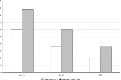
most reliable borrowers.8 And, while microlenders may still find a pool of customers after real interest rates are raised, the customers may not be from the same pool that was willing and able to pay the lower rates. Fears like these, coupled with a strongly-felt moral imperative to keep costs as low as possible for the poor, have compelled the larger microlenders in Bangladesh to keep real interest rates below 40 percent per year, even if it means turning to subsidized resources to cover costs (e.g., Morduch, 1999). Figure 1 shows that the average fees charged by two large lenders in Bangladesh are just under 30 percent. The Grameen Bank (which is not one of the two) keeps their interest rates and fees close to 20 percent per year (nominal) on their main lending products—and they deflect suggestions to raise rates. Figure 2 shows differences in real interest rates across continents, with South Asia at the low end. Figure 3 shows that institutions serving the poorest customers tend also to charge higher interest rates and face higher costs relative to lenders serving clients upmarket.

3. The SafeSave Program

About one third of Dhaka’s 11 million people live in slums. Most adult slum residents are poor but working, finding informal sector jobs such as being a driver, domestic help, or construction worker. Some find work in factories, particularly in the garment industry. The slums have active economies of their own, but they are poorly served by formal financial intermediaries. Instead, traditional means of saving and borrowing, like joining rotating saving and credit associations (ROSCAs) or finding a friend willing to serve as a “money guard”, are common ways to manage funds.9

SafeSave was launched in 1996 with the mission of offering its clients “the most

convenient possible way to turn their savings into usefully large sums of money.”10 To do this, SafeSave clients are served by “collectors” who visit them in their homes or businesses six days a week. Each day, clients can choose to add to their savings, pay down loans, or to draw down their savings, in amounts that are variable and freely chosen. Clients must visit the branch office only to withdraw more than 500 taka in a day or to get a loan. Once clients obtain a loan, they can pay it back on their own

schedule – in small frequent bits, in a lump sum, quickly, or stretched out over time. The only stipulation is that interest on the outstanding balance must be paid each month. The program thus combines the convenience of a ROSCA with the flexibility that a bank can offer. While borrowers are required to hold savings accounts, savers are not

required to borrow; at any time, about two thirds of clients hold loans. None of the loans require assets to be pledged as collateral, although, as we describe below, a form of “financial collateral” is employed.11

The first branches were in western Dhaka. Apart from residence in the slum, there are no additional eligibility requirements or means tests. The first branches served were in Tikkapara and Kalyanpur, a mix of densely-populated slums where squatters live in rows of lightweight huts built on bamboo frames, with woven bamboo walls and, in better circumstances, tin roofs. The third branch was opened in Geneva slum, a

community of Bihari refugees with government-provided concrete housing along a grid of

8 _{The arguments are reviewed in Armendariz and Morduch (2005). McKenzie and Woodruff (2003) give}

evidence from Mexico that shows no signs of non-convexities in production for small-scale entrepreneurs.

9 _{Rutherford (1997) describes a survey of informal finance in the Dhaka slums. Half of the sample, collected}

from financial diaries described in Rutherford (2004), is from the Dhaka slums. Both studies provide rich data on a relatively small sample. In contrast, the present study takes advantage of a large sample but just a limited number of variables.

10 _{The quote is taken from www.safesave.org in April 2004.}

narrow lanes. The analysis below compares interest rate changes in Tikkapara and Kalyanpur to ongoing conditions in Geneva.

4. The Data

After making their daily rounds to the homes and businesses of their customers, the records of SafeSave collectors are entered into database software for use by management. We use the daily data to calculate basic measures of saving and borrowing and then aggregate them to the monthly level. Most of the variation in loan balances occurs between months, rather than within, so little relevant information was sacrificed through aggregation. In addition to financial variables, we also know the customers’ ages, gender, and length of time with the bank. Given the long time-series dimension, we can control for time invariant unobservables using fixed effects.

Most of the analysis focuses on 68,037 month-customer observations between January 1999 and January 2001. They reflect data on 5,147 customers, not all of whom are part of the program during the entire period. The change in the interest rate occurs midway through the sample, in February 2000.

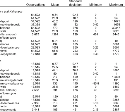
Table 1 provides summary statistics for the sample, restricted to the dates we study. Two thirds of the clients are women (or girls), with an average age in the late twenties. The financial data show that in all three branches, monthly deposits to savings are small, averaging about 55 taka (or $2.53 in January 2000 US dollars). In Tikkapara and Kalyanpur, which had started several years before Geneva, accumulated savings balances averaged 579 taka (or $26), while in Geneva the average savings balance was 217 taka (or $10). Average loan sizes are small relative to those from other

microlenders (at 1051 taka, or $48, in Tikkapara and Kalyanpur and 891 taka, or $37, in Geneva). Loan balances (which reflect partial repayments) are similar in the branches – about 434 taka ($20) in Tikkapara and Kalyanpur and 480 taka (or $22) in Geneva. The typical length of a loan cycle is short, approximately one month between the time a loan is taken and repaid. Each repayment is relatively small, 200 taka (or $9.25) in Tikkapara and Kalyanpur and 405 taka (or $18.66) in Geneva, corresponding on average to repaying a quarter of the loan each week or half every two weeks.

5. Estimation and Identification

Identification of the impact of the February 2000 interest rate increase (from 2 percent per month to 3 percent per month) exploits the fact that the change occurred in Tikkapara and Kalyanpur branches, but not in Geneva Branch. Geneva had already started with an interest rate of 3 percent per month when it opened in March 1999.

Identification hinges on the presumed lack of correlation of the timing of the interest rate change with other events occurring in Tikkapara and Kalyanpur. Based on interviews with the bank, the timing of the switch seems to have been both arbitrary and unexpected.12 Contemporaneous changes that occur in all three branches will be controlled for through the inclusion of data from Geneva branch and the estimation of baseline trends using those data.

This setup suggests a difference-in-difference estimator, although there is one feature that merits particular attention here. Unlike a situation in which customers move from one equilibrium to another with little else in the environment changing but the price,

12 _{As Stuart Rutherford, the founder of SafeSave, remembers the switch: “It was fairly arbitrary… I don't}

here customers are steadily building up savings and the capacity to borrow. New

customers are also joining, and some older customers are beginning to depart. Because we have records for all customers, past and present, concern with attrition is limited here, but we pay close attention to the underlying upward trends in borrowing and saving. It is against those trends that we see a reduction of demand for borrowing. The net effect we will find is a slowing down in the rate of borrowing in the year following the interest rate increase.

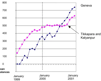
The basic trends can be seen in Figure 4, which gives average monthly loan balances in Geneva Branch versus Tikkapara and Kalyanpur combined. Since Geneva started only in March 1999, we find a steady rise from zero upward, whereas growth in the other two branches starts at a higher level and flattens in the middle of the period. The vertical line marks January 2000, the month prior to the interest rate increase. It is notable that in 1999 both groups have a similar, linear trend. This suggests that the differences-in-differences assumption is plausible. Hence, we begin with a simple difference-in-difference specification:

yit = β0 + β1Treatedi+ β2Postt + β3Treatedi×Postt + εit (1)

where: i indexes clients and t the month; yit is the dependent variable (typically average monthly loan balances, but also an indicator for loans, amount loaned, and repayments);

Treatedi takes on a value of 1 for individuals in Tikkapara and Kalyanpur and 0 for those

in Geneva; and Postt refers to time periods after the interest rate increase. Hence, β3

gives the impact of the interest rate increase: the change in borrowing before and after the interest rate increase in Tikkapara and Kalyanpur, relative to the contemporaneous change in Geneva.

We proceed to refine this estimation strategy along a number of dimensions. First, we control for borrower characteristics, including age and length of time in the program. Second, rather than simply controlling for time effects with a before-versus-after dummy, we include a full set of month-year dummies. Third, we include account fixed effects; this then controls for all non-time-varying differences among borrowers. Fourth, we allow for trend differences between the treated and comparison groups, in addition to a shift in the level of borrowing. Finally, the basic setup is expanded to consider the heterogeneity of responses (along dimensions such as gender, wealth, and age).

We extend these results with an alternative specification that uses knowledge of

SafeSave’s product rules to control for credit supply. In particular, we use the exact formula used by SafeSave to determine and control for an individual’s maximum

borrowing capacity. For example, in Tikkapara and Kalyanpur, borrowers are not allowed to borrow until they have been customers for at least two months and their savings have reached 500 taka (just under $10 in January 2000).13 At that point they can borrow their saving balance plus 1000 taka. The next time, they can increase the loan size by another 500 taka, and so on, without limit, adding another 500 taka to their credit limit with each successive cycle. (The exact rules are in the appendix.)

This is an important advantage of the data we are using because individuals might respond differently to changes in the interest rate based on their ability to borrow. For example, individuals with low (or zero) borrowing capacity cannot significantly respond to changes in interest rates. Since borrowing capacity hinges in part on savings behavior, and since savings behavior is likely to be jointly determined with borrowing, there is a fear that simultaneity and, possibly, omitted variables will bias the results. We thus instrument for capacity using the length of time the accountholder has been with the bank. Time in program is a valid instrument for capacity under three assumptions, all of

which seem reasonable for our data: exogeneity (since time in program increases linearly it is unlikely to be correlated with simultaneous shocks to borrowing and saving), relevance (the longer individuals are in the program typically the more savings they accumulate), and exclusion (assuming we have correctly computed borrowing capacity, which is reasonable since we observe all the information that the bank does, then the only reason that time in program should affect borrowing is through savings and in turn capacity).

6. Results

6.1 Diffs-in-diffs and fixed effects

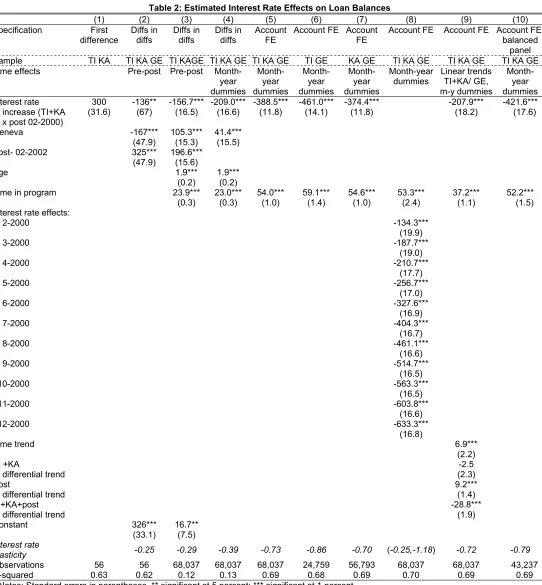
The first column of Table 2 gives the results of a simple difference in loan balances before and after the interest rate increase in Tikkapara and Kalyanpur. The coefficient is positive, reflecting the upward trend in overall loan balances (as seen in Figure 4). The basic differences-in-differences estimator (column 2) uses Geneva to estimate and subtract off this trend; the net impact of the interest rate increase is a 136 taka reduction in loan demand. The impact is small (the implied elasticity is -0.25) but, given the large sample size, statistically significant.

The interest rate elasticity falls (to -0.29) once customer age and their time with the bank are included as controls in the third column. The fourth column increases the flexibility of the specification by allowing for a full set of month-year dummy variables. The ability to better control for underlying trends lowers the interest rate elasticity further, to -0.39.

Few controls for heterogeneity in customer tastes and constraints are available in the data, but the long time series dimension of the panel allows precise estimation of account fixed effects. Adding controls for account fixed effects in column 5 absorbs a significant amount of variation (the R-squared increases from 0.13 to 0.69) and reduces the interest rate elasticity to -0.73. The next two columns show that the elasticities are in a similar range when estimated for Tikkapara (-0.86) and Kalyanpur (-0.70) separately. The eighth column of Table 2 allows the estimated impacts to vary by month; we see that the immediate responsiveness is small (an elasticity of -0.18), but increases substantially over time (to -1.18 a year after the change). The ninth column allows trends in Tikkapara and Kalyanpur to differ from Geneva’s base trend both before and after the interest rate change (we retain the differential intercepts of the standard diffs-in-diffs model, in addition to account fixed effects). The treatment effect in this model is both the shift in the intercept and the differential trend associated with being in Tikkapara or Kalyanpur in the months after the interest rate increase. The average elasticity in this specification is -0.72, which is in the same range as the previous results.

The panel used above is not balanced: customers enter the program at different points and some exit before January 2001. One concern is that the changing mix of customers over time affects the results. So, in column 10, we restrict attention to a balanced panel made up of customers who are in the panel for at least six months prior to the February 2000 interest rate increase. These estimates from the balanced panel yield similar results to the base specification in column 5; the estimated interest rate elasticity is -0.79.

6.2 Heterogeneous effects

In this subsection we examine the heterogeneity of our main result along three dimensions: estimation window, lower wealth versus higher wealth, and borrowing capacity.

6.2.1 Estimation window

We begin by examining how the choice of estimation window affects our results. In our main results, we include the period 12 months before and after the change in interest rates. The concern is that with a longer estimation window trends in the data could be driving the results. Thus in Table 3, columns 1 and 2, we narrow the window to nine months and to three months before and after the policy change. Dropping the last three months of our sample is useful because of the apparent increase in the growth of loans seen in Tikkapara and Kalyanpur in Figure 4 at the end of the sample period. For the narrower window, the estimated elasticity is -0.7, similar to our baseline estimate. In column 2, for the narrowest window, the estimated responsiveness is smaller, though still negative and significant at standard levels. The elasticity in this specification is -0.37.

6.2.2 Lower-wealth versus higher-wealth borrowers

In the next three columns, we investigate how wealth affects the impact of interest rates on loan balances. Without a comprehensive measure of wealth, we turn to data on average saving balances. In column 3, the sample is restricted to households who did not save at least 100 taka during one of the months between June 1999 and August 1999,14 _{and the estimation window is restricted to October 1999 to January 2001.}

Column 4 considers households who saved over 100 taka during any month in the June to August period. The estimates show that the “low-saving” group is more responsive to the interest rate than the “highsaving” group, with an elasticity of 0.86 compared to -0.26. We conclude that the composition of SafeSave’s loan portfolio shifted toward (relatively) wealthier clients compared to the composition before the increase.

We examine this effect directly in column 5 where we estimate the effect of the interest rate change on size of loans taken by poor borrowers. We use a

triple-differences estimator: we are comparing the growth in the amount loaned to the poor relative to the rich in Tikkapara and Kalyanpur, before and after the interest rate

increase, subtracting out the same difference from Geneva to control for the time trend. We find that there was a 250 taka decrease in the typical size of loan taken by poor borrowers because of the interest rate change, a decrease of 12 percent relative to the mean. Note that the decrease in amount loaned is relative to Geneva. In absolute terms, the amount loaned to the poor relative to the rich decreased in Tikkapara and Kalyanpur by 624 taka, compared to a decrease of 373 in Geneva over the same period.

We also explored possible differences in responsiveness by gender and age (in specifications not reported here), but do not find substantial differences in estimated elasticities.

6.2.3 Borrowing capacity

Table 2 presented a range of estimates of the change in loan balances in response to changes in the interest rate. Though these estimates account for time trends, time effects more flexibly, and observed and unobserved individual characteristics, the

14 _{Alternative definitions, based on cash inflows (did the customer make deposits or repay loans in amounts}

estimates do not account for variation in borrowing capacity. In particular, individuals with low borrowing capacity are less able to respond to changes in interest rates than individuals with higher capacity (this is most transparent for individuals with zero borrowing capacity). In columns 6 and 7 we address this by taking advantage of our knowledge of the rules used by SafeSave to determine the maximum loan capacity of borrowers (the rules are detailed in the appendix).

Column 6 introduces capacity as a control in our main specification. The estimated interest-rate responsiveness and elasticity are somewhat greater than our baseline result, -0.88 compared to -0.73. The coefficient on capacity is 0.2, which suggests that households increase their borrowing by only 20 percent of an increase in borrowing capacity.

However, measurement error, simultaneity, and omitted variable bias with respect to the capacity measure are serious concerns. Though in principle we measure borrowing capacity precisely, there is always scope for some variation in a branch’s loan decision. There is also a serious concern of simultaneity. A common shock could drive both savings (which is the most important component of capacity) and borrowing. In particular, the presumption is that a negative shock would decrease savings and increase the demand for loans, potentially biasing our results downward. Finally, borrowing capacity is determined mostly by savings, which could affect the demand for loans for reasons other than borrowing capacity.

We address all of these concerns by instrumenting for loan capacity using the length of time the individual has been in the program. As discussed in Section 5, time in program plausibly satisfies the key requirements for a valid instrumental variable. Results are presented in column 7. We note that the F-statistic of the instrument in the first stage is reasonably high (10.75). The estimated effect of interest rates on borrowing increases in absolute value. The implied interest rate elasticity is now -1.04, the lowest elasticity that we find in any specification.

6.3 Mechanisms

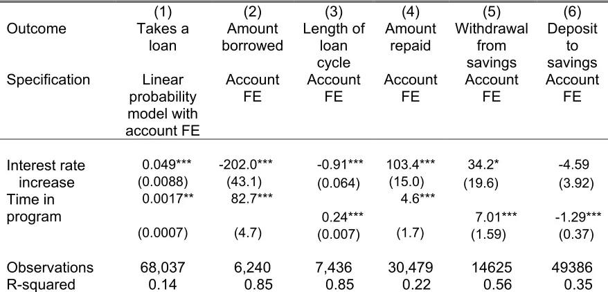
Several mechanisms could account for our results: reductions in the probability of taking loans, reductions in the size of those loans, increased speed in repaying loans, or some combination of these. In Table 4 we examine each of these outcomes using our base specification.

In column 1 we begin by considering a linear probability model where the

dependent variable is a dummy variable for whether the borrower takes a loan in a given month. We find a five percentage point increase in the probability of taking a loan. If borrowers are taking more loans, but average loan balances are decreasing, it would suggest either that the size of loans is decreasing or that repayment rates are

accelerating. Columns 2, 3, and 4 show that both of these are the case. We find that the amount borrowed decreases by about 17 percent relative to the typical loan size. For the amount repaid, we find an increase of approximately 100 taka, or 60 percent relative to the typical monthly repayment. At the same time, the time between loans fell by about one month, suggesting that the interest rate increase induced borrowers to take more frequent, smaller loans and to repay them more quickly than before.

7. Conclusion

We have examined the widely held view that the loan elasticity of demand in

microfinance institutions is low. The goal of reaching as many unbanked customers as possible has pushed microlenders to pursue profitability. Once profitable, microlenders can expand as far as the market will allow, without concern for the availability of funds from donors. The natural fear, though, is that raising interest rates too high will erode surpluses generated by customers and reduce the demand for financial services, undermining the original intention of the push for microfinance. This concern has, however, been largely ignored, with the argument that poor customers are apt to be insensitive to interest rates and have ample surpluses with which to pay cost-covering fees. We examine this tradeoff in the context of SafeSave, a microfinance organization operating within the slums of Dhaka.

Appendix:

SafeSave product rules15 Product P2

Offered in Tikkapara and Kalyanpur branches as of November 1997. Not changed (except for the February 2000 interest rate rise on loans) until August 2003.

Eligibility: Anyone in the slum including children (children allowed to borrow); multiple accounts per person allowed and per household allowed.

Account Fees: no account opening, closing, or monthly fees.

Savings: Deposit any sum any time; withdraw any sum any time unless a loan is held in which case no withdrawal allowed; interest paid in two ways (a) if account held for 5 years, then 25 percent of final balance paid at the end of the term (provided certain safeguards against ‘end loading’ were satisfied) (b) if account closed before 5 years interest paid retrospectively at closure at 1 percent a month for accounts that attained and maintained 1000 balance.

Loans: Account must be 2 months old and savings must have reached 500 before first loan; first loan = savings balance + 1000, subsequent loans savings balance + 1500, then savings balance + 2000, etc, no limit; disbursement fee of 100 for loans up to 5000, 200 taka for bigger ones; interest charged monthly at 2 percent per month on

outstanding balance at end of previous month; no fixed repayment schedule and no fixed term but a ‘renewal fee’ equal to the disbursement fee payable each 6 months.

In February 2000, the interest rate on loans was raised from 2 percent to 3 percent per month; renewal fees set at 3 percent of outstanding balance (rather than as a set figure).

Insurance: None.

Product P3

Only offered in Geneva branch. Introduced in March 1999 and not changed until August 2003.

Eligibility: Anyone in the slum including children (children allowed to borrow); multiple accounts per person allowed and per household allowed.

Account Fees: no account opening or closing fees, 10 taka monthly service fee.

Savings: Two products: current and long-term, both optional.

Current Savings: deposit any sum any time; withdraw any sum any time; no linkage with

loans; interest paid on balances of 500 or more at 1 percent a month but no interest in months when withdrawals are made.

15 _{These rules were written by Stuart Rutherford. Kalyanpur was originally served by the Tikkapara branch}

Long-term savings: a 60-month accumulating savings device, monthly deposits 50 or a multiple of 50; if terminated prematurely no interest is paid; after 60 months the client stops saving and interest is added at the same monthly deposit rate, so the longer the client holds the savings the more s/he receives and the higher the effective rate.

Loans: Client must have held and paid into a long-term savings account for 2 months before a loan can be taken, and must be up-to-date with long-term savings to borrow; first loan value 1000 then rises in 1000 steps; maximum value cannot exceed the monthly long-term deposit x 100. Repay any time, any schedule; charge of 3 percent of loan when it is disbursed; interest paid monthly at 3 percent of previous month-end balance.

References

Adams, Dale W., Douglas H. Graham, and J. D. von Pischke, eds. (1984). Undermining

rural development with cheap credit. Boulder, CO, USA: Westview Press.

Armendariz de Aghion, Beatriz and Jonathan Morduch (2005). The Economics of

Microfinance. Cambridge, MA: MIT Press.

Consultative Group to assist the Poorest [CGAP] (1996), “Microfinance Interest Rates,”

Occasional Paper No. 1.

David, Cristina (1984). “Credit and price policies in Philippine agriculture” ch. 17 in Dale W. Adams, Douglas H. Graham, and J. D. von Pischke, eds. (1984).

Undermining rural development with cheap credit. Boulder, CO, USA: Westview

Press.

Drake, Deborah and Elisabeth Rhyne, eds., (2002). The Commercialization of

Microfinance: Balancing Business and Development. Bloomfield, CT: Kumarian

Press

Gross, David and Nick Souleles (2002). “Do Liquidity Constraints and Interest Rates Matter for Consumer Behavior? Evidence from Credit Card Data,” Quarterly

Journal of Economics, February: pp. 149-185.

Homer, Sidney and Richard Sylla (1996), A History of Interest Rates, 3rd ed. New Brunswick, NJ: Rutgers University Press.

Karlan, Dean and Jonathan Zinman (2005). “Observing Unobservables: Identifying Information Asymmetries with a Consumer Credit Field Experiment,” Princeton University and Federal Reserve Bank of New York, working paper.

Laffont, Jean-Jacques and Patrick Rey (2003). “Collusion and Group Lending with Moral Hazard,” draft, IDEI, Toulouse and University of Southern California.

McKenzie, David and Christopher Woodruff (2003). “Do entry costs provide an empirical basis for poverty traps? Evidence from Mexican microenterprises.” BREAD Working Paper No. 020, February. [Available at

www.cid.harvard.edu/bread/papers/020.pdf]

McKinnon, Ronald (1973). Money and Capital in Economic Development. Washington, DC: The Brookings Institution.

Morduch, Jonathan (1999), “The Role of Subsidies in Microfinance: Evidence from The Grameen Bank,” Journal of Development Economics 60, October: 229 - 248.

New York Times, “Micro-Loans for the Very Poor”, February 16, 1997. Editorial

Robinson, Marguerite (2001). The Microfinance Revolution. Washington, DC: The World Bank.

Rutherford, Stuart (1997). “Informal Financial Services in Dhaka's Slums,” ch. 16 in Geoffrey Wood and Iffath Sharif, eds., Who Needs Credit? Poverty and Finance

in Bangladesh. Dhaka: The University Press Limited.

Rutherford, Stuart (2000). The Poor and Their Money. New Delhi: Oxford University Press.

Rutherford, Stuart (2004). “Money Talks: Conversations with Poor Households in Bangladesh about Managing Money,” Journal of Microfinance.

Sayad, João (1983). “The Impact of Rural Credit on Production and Income Distribution in Brazil”, chapter 45 in J. D. von Pischke, Dale Adams, and Gordon Donald, eds., Rural Financial Markets in Developing Countries. Baltimore: Johns Hopkins for the World Bank.

Stiglitz, Joseph (1990). “Peer Monitoring and Credit Markets” World Bank Economic

Figure 1: Real Yields on Gross Portfolio, Country averages

MicroBanking Bulletin, July 2003 (n = 124)

0 10 20 30 40 50 60 70 80 Yugo slav ia Cro atia Alba nia Beni n Togo Sene gal Gua tem

ala _India

Bosn ia a

nd H erzo

govi na

Cos ta R

ica Bang lade sh Nic arag ua Leba non Mon golia Wes t Ban

k an d G

aza Braz il Moz ambi que Sout h Af

rica Jord an Geo rgia Uga nda Indo nesi a Mex ico Arm enia

Figure 2: Real Yields on Gross Portfolio, Region averagesand maximums

MicroBanking Bulletin, July 2003 (n = 124)

0 20 40 60 80 100 120

Africa (21) Middle East and N. Africa E. Asia and the Pacific (11) Latin America and the South Asia (12)

Maximum

Figure 3: Total expense ratio and real gross portfolio yield, by target group

MicroBanking Bulletin, July 2003 (n=124)

Notes: “Low-end” institutions include those with a ratio of average loan size to GNP per capita below 20 percent (or an average loan size under US$150). For “broad”

institutions, the ratio is between 20 percent and 149 percent, and for “high-end” institutions, it is between 150 percent and 249 percent. The total expense ratio is the ratio of total expenses to assets.

0 5 10 15 20 25 30 35 40 45 50

Low-end Broad High

Figure 4: Average loan balances, SafeSave

0 100 200 300 400 500 600 700 800

Loan balances

Geneva

Tikkapara and Kalyanpur

January 2000

January 2001 January

Table 1: Descriptive Statistics

Monthly averages, January 1999 – January 2001

Observations Mean

Standard

deviation Minimum Maximum

Tikkapara and Kalyanpur

Female 54,522 0.64 0.48 0 1

Age 54,522 26.9 10.7 4 94

Saving deposit 54,522 43.2 128 0 11675

Positive saving deposit 36,358 65 152 0.42 11676

Saving balance 54,522 579 978 0 30347

Withdrawals 54,522 26.9 159 0 9823

Loan (initial amount) 3,675 1384 729 424 6446

Length of loan cycle

(months) 54,522 0.81 1.13 0 10

Loan balances 54,522 434 665 0 6501

Positive loan balances 22,523 1051 650 0.22 6501

Repayments 54,522 65.6 223 0 4772

Positive repayments 17.813 201 353 0.43 4772

Geneva

Female 13,515 0.67 0.47 0 1

Age 13,515 27.5 10.7 2 94

Saving deposit 13,515 44.1 76.8 0 1880

Positive saving deposit 11,848 50 80 0.42 1

Saving balance 13,515 217 409 0 13803

Long-term saving deposit 13,515 23.3 17.6 0 131

Long-term saving balance 13,515 136 145 -85.8 1190

Withdrawals 13,515 36.5 129 0 6489

Loan (initial amount) 2,568 891 476 43 3393

Length of loan cycle

(months) 13,515 1.30 1.36 0 80

Loan balances 13,515 480 545 0 3365

Positive loan balances 7,956 816 481 3.16 3365

Repayments 13,515 103 276 0 3887

Positive repayments 3,443 405 421 2.15 3887

Table 2: Estimated Interest Rate Effects on Loan Balances

(1) (2) (3) (4) (5) (6) (7) (8) (9) (10)

Specification First difference Diffs in diffs Diffs in diffs Diffs in diffs Account FE

Account FE Account FE

Account FE Account FE Account FE, balanced

panel

Sample TI KA TI KA GE TI KAGE TI KA GE TI KA GE TI GE KA GE TI KA GE TI KA GE TI KA GE

Time effects Pre-post Pre-post

Month-year dummies Month-year dummies Month- year dummies Month-year dummies Month-year dummies Linear trends TI+KA/ GE, m-y dummies Month- year dummies

Interest rate 300 -136** -156.7*** -209.0*** -388.5*** -461.0*** -374.4*** -207.9*** -421.6***

increase (TI+KA x post 02-2000)

(31.6) (67) (16.5) (16.6) (11.8) (14.1) (11.8) (18.2) (17.6)

Geneva -167*** 105.3*** 41.4***

(47.9) (15.3) (15.5)

Post- 02-2002 325*** 196.6***

(47.9) (15.6)

Age 1.9*** 1.9***

(0.2) (0.2)

Time in program 23.9*** 23.0*** 54.0*** 59.1*** 54.6*** 53.3*** 37.2*** 52.2***

(0.3) (0.3) (1.0) (1.4) (1.0) (2.4) (1.1) (1.5)

Interest rate effects:

2-2000 -134.3***

(19.9)

3-2000 -187.7***

(19.0)

4-2000 -210.7***

(17.7)

5-2000 -256.7***

(17.0)

6-2000 -327.6***

(16.9)

7-2000 -404.3***

(16.7)

8-2000 -461.1***

(16.6)

9-2000 -514.7***

(16.5)

10-2000 -563.3***

(16.5)

11-2000 -603.8***

(16.6)

12-2000 -633.3***

(16.8)

Time trend 6.9***

(2.2)

TI +KA -2.5

differential trend (2.3)

Post 9.2***

differential trend (1.4)

TI+KA+post -28.8***

differential trend (1.9)

Constant 326*** 16.7**

(33.1) (7.5)

Interest rate

elasticity -0.25 -0.29 -0.39 -0.73 -0.86 -0.70 (-0.25,-1.18) -0.72 -0.79

Observations 56 56 68,037 68,037 68,037 24,759 56,793 68,037 68,037 43,237

R-squared 0.63 0.62 0.12 0.13 0.69 0.68 0.69 0.70 0.69 0.69

Table 3: Heterogeneity of Estimated Interest Rate Effects on Loan Balances

(1) (2) (3) (4) (5) (cut) (6) (7)

Outcome Loan balances Loan balances Loan balances Loan balances Amount loaned to poor Loan balances Loan balances Loan balances

Specification Account FE Account FE Account FE Account FE Diffs in diffs(b)

OLS OLS IV(d)

Sample April 1999

to October 2000 November 1999 to May 2000 Low savings(a) High savings

TI KA vs. GE

Capacity>0 All All

Interest rate increase

-373.3*** -198.1*** -331.0*** -169.6*** -250*** -400.6 -469.5 -555.7

(11.4) (11.8) (12.1) (35.5) (129) (14.7) (9.9) (13.1) Borrowing

capacity(c)

0.2 0.44

(0.001) (0.011)

Time in program

50.8*** 64.1*** 54.5*** 30.9*** 59.1 35.7

(0.8) (2.1) (1.4) (4.0) (2.1) (0.8)

Interest rate elasticity of borrowing

-0.70 -0.37 -0.86 -0.26 -0.75 -0.88 -1.04

F-stat in

instrument 10.75

Observations 53156 19719 31,291 20,318 6,243 36,231 68,037 68,037

R-squared 0.73 0.87 0.69 0.78 0.25 0.68 0.78 0.78

Notes: Standard errors in parentheses. All coefficients are statistically significant at 1 percent.

(a) Low-savings individuals are identified using savings balances between June to August 1999, and the subsequent responsiveness to the change in interest rate is measured using data from October 1999 on.

(b) This is a triple-differences specification, looking at the change in Tikkapara and Kalyanpur in amount loaned to poor individuals after the interest rate change compared to before the interest rate change, relative to the same difference for rich individuals in Tikkapara and Kalyanpur, subtracting out the before-after rich-poor difference from Geneva.

(c) Borrowing capacity uses program rules in conjunction with savings to determine the maximum amount an individual could borrow.

Table 4: Estimated Interest Rate Effects, Further Results

(1) (2) (3) (4) (5) (6)

Outcome Takes a

loan

Amount borrowed

Length of loan cycle

Amount repaid

Withdrawal from savings

Deposit to savings Specification Linear

probability model with account FE

Account FE

Account FE

Account FE

Account FE

Account FE

Interest rate 0.049*** -202.0*** -0.91*** 103.4*** 34.2* -4.59

increase (0.0088) (43.1) (0.064) (15.0) (19.6) (3.92)

Time in program

0.0017** 82.7***

0.24***

4.6***

7.01*** -1.29***

(0.0007) (4.7) (0.007) (1.7) (1.59) (0.37)

Observations 68,037 6,240 7,436 30,479 14625 49386

R-squared 0.14 0.85 0.85 0.22 0.56 0.35

Notes: All specifications contain month-year dummies.