Nonparametric estimation of time varying covariance matrix in a slowly changing vector random walk model

Munich Personal RePEc Archive

Nonparametric estimation of

time-varying covariance matrix in a

slowly changing vector random walk

model

Feng, Yuanhua and Yu, Keming

Heriot-Watt University and Brunel University

2006

Online at

https://mpra.ub.uni-muenchen.de/1597/

Nonparametric Estimation of Time-Varying Covariance Matrix

in a Slowly Changing Vector Random Walk Model

Yuanhua Feng

Department of Actuarial Mathematics and Statistics, Heriot-Watt University

and Keming Yu

Department of Mathematical Sciences, Brunel University

Abbreviated Title: Slowly changing vector random walk

Summary. A new multivariate random walk model with slowly changing

pa-rameters is introduced and investigated in detail. Nonparametric estimation of

local covariance matrix is proposed. The asymptotic distributions, including

asymptotic biases, variances and covariances of the proposed estimators are

ob-tained. The properties of the estimated value of a weighted sum of individual

nonparametric estimators are also studied in detail. The integrated effect of

the estimation errors from the estimation for the difference series to the

inte-grated processes is derived. Practical relevance of the model and estimation is

illustrated by application to several foreign exchange rates.

Keywords: Multivariate time series; slowly changing vector random walk; local covariance matrix; kernel estimation; asymptotic properties; forecasting.

AMS 2000 subject classifications: Primary 62G08; Secondary 62M10

1

Introduction

Random walk models, including Weiner processes or Brownian motion arise in many

appli-cations, particularly in financial time series, statistical physics, genetics, graphs, modelling

of turbulent dispersion within the atmosphere and to geographic distributions of animal; see

Kijima (2002), Weiss (1994), Neigel and Avise (1993) and Lov´asz (1993). In these

applica-tions often an analysis of the relaapplica-tionships between more than one variable simultaneously

is required. Vector (also called multiple or multivariate) random walk is the simplest

1989). Such a model can be used for modelling financial difference or return series which

is also often used to built some more complex models. In Harvey et al. (1994) vector

random walk is used to model persistent movements in stochastic volatility models. Due to

slow change of economic or environmental situations however the means and variances, also

the covariances and correlations between the components of the innovation process may

all change slowly over time. In this paper a slowly changing vector random walk model is

hence introduced to model the slowly change multiple time series.

The paper is organized as follows. Section 1.1 reviews the existing literature on stochastic

time varying process. Section 1.2 presents a motivating example involving exchange rate.

The multivariate random walk model with slowly changing parameters is introduced in

Section 2. Nonparametric inference methods for time-varying covariance matrix are defined

in Section 3. Properties of the estimators are derived in Section 4, including asymptotic

mean square errors and optimal bandwidth. An optimal prediction of the future value of a

portfolio is developed in Section 5. Practical performance of the proposed methods through

an application to four daily foreign exchange rate is discussed in Section 6. Concluding

remarks are presented in Section 7 and the proofs can be found in Appendix.

1.1 A brief review of closely related research

Univariate locally stationary processes were first introduced and studied by Dahlhaus (1997,

2000). Nonparametric inference for the mean and variance functions in univariate stochastic

process has attracted much attention in statistics literature. We list few of a rich literature

using in this context. Kernel regression estimation with time series errors is studied e.g.

by Hart (1991) and Cs¨og¨o and Milnikzug (1995). Beran and Ocker (1999) and Beran and

Feng (2002) discussed nonparametric trend estimation in integrated processes. Fan and

Yao (1998) proposed nonparametric estimation of conditional variance function following

the idea of the ARCH (autoregressive conditional heteroskedasticity, Engle, 1982) model.

A¨ıt-Sahalia (1996) studied nonparametric estimation of time-varying drift and diffusion

coefficients of a Brownian motion.

In contrast to univariate models, which model each component independently,

vast literature on parametric multivariate GARCH (generalized ARCH) models for

condi-tional covariance matrix (see e.g. Bollerslev et al., 1988 and Engle, 2002) and on

nonpara-metric estimation of conditional covariance matrix (H¨ardle et al., 1998, 2003). However in

this paper we will focus on the estimation of covariance matrix in a slowly changing model.

The slowly change in the current model means some deterministic components which are

non-stochastic. The real examples in Section 1.2 clearly illustrate the phenomenon of slow

change. Actually, in the new model named SCVRW model the change in the means,

vari-ances, covariances and correlations is assumed to be deterministic not conditional. They

change smoothly over time and do not depend on the past information. This is what slow

change means. On the other hand conditional changes in such components are caused by

past observations. Conditional changes and local changes can not explained each other.

Despite a huge number of literature on the estimation of conditional covariance matrix,

little research on the estimation of local covariance matrix can be found in literature. Herzel

et al (2006) explores some ideas on volatility estimation under a non-stationary multivariate

return model, but assumes a constant drift term, lacks theoretical investigation and ignores

forecasting in depth. Wu and Pourahmadi (2003) discussed nonparametric estimation of

the covariance matrix of the observations of a univariate time series based on Cholesky

decomposition, where it is proposed to estimate the diagonal matrix with the variances as

its diagonal entries and the unit lower triangle matrix using local polynomial separately.

1.2 Motivation examples

The slow change economics phenomenon can be observed in finance such as the indices of

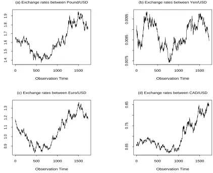
major stock markets and exchange rates. Figure 1 displays the scatter plots of four daily

foreign exchange rate series w.r.t. the US Dollar (USD). The data are those of the British

Pound (Pound), Japanese Yen (Yen), Euro and Canadian Dollar (CAD), from 4 January

1999 to 4 November 2005. Here the USD price per foreign currency is used. Figure 1

shows that there are clear non-constant drifts in these series which change slowly over time.

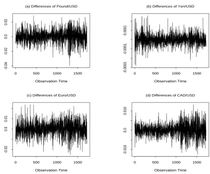
Figure 2 displays the difference series of the original data from which we can see that the

variances of the difference series change clearly over time. What cannot be discovered by

(see Figure 6 in Section 6). This can also be shown graphically by plotting two difference

series against each other piece by piece.

For this data and the content in finance, one is concerned

(a) how to model properly the slowly changing drifts, variance and correlation coefficients

of underlying stochastic process,

(b) what is the estimation of the mean and variance of a portfolio, and

(c) what is the effect of estimation errors in the short term forecasts.

Other slowly change multivariate time series include ice thickness series. It is widely

concerned that global warming results in quickly decreasing ice-thickness. However, the

ice thickness series are random walks (the sum of snow fall years after years). There is a

nonparametric trend in the differences of these data, because of the different strength of

press (or maybe also other reasons), the dependence between ice thickness in different years

(after removing the trend) is very weak. In all, different series of ice thickness may also be

able to be modelled using the SCVRW.

Global and hemispheric series of temperature anomalies can also be modelled by random

walks (Gorden, 1991). Similarly, statistical analysis for satellite-based global daily

tropo-spheric and stratotropo-spheric temperature anomaly and solar irradiance data sets shows that

the behavior of the series appears to be nonstationary with stationary daily increments

(K¨arner, 2002). The model proposed in this paper provides a useful tool for modelling

global warming as slow change in the increments of those series.

2

The model

Let Yt be a k-dimensional stochastic process, andY0 be the initial value ofYt. LetCbe

a constant vector, and let Zt be the increment of Yt.

The proposed slowly changing vector random walk (SCVRW) is defined by

        

Y0 = C,

Yt = Yt−1+Zt fort= 1,2, ..., n,

Zt = µ(xt) +Σ1/2(xt)Et,

where

Yt=

    

Y1t

.. . Ykt    

, Zt=

    

Z1t

.. . Zkt    

, Et=

    

ǫ1t

.. . ǫkt     

are random vectors, xt=t/n is the re-scaled time,

µ(xt) =

    

µ1(xt)

.. .

µk(xt)

   

 and Σ(xt) =

    

σ₁2(xt) · · · σ1k(xt)

..

. . .. ...

σk1(xt) · · · σ2_k(xt)

   

 (2)

are the vector of local mean functions and the matrix of local variances or cross-covariance

functions, respectively, and Σ1/2 denotes lower triangular Cholesky factorization of a

semi-positive definite matrix so that

Σ=Σ1/2Σ1/2′.

For convenience we will also denote σ_i2(xt) by σii(xt), i = 1, ..., k. It is assumed that

σii(·) are strictly positive for all i and that ǫit given i are i.i.d. N(0,1) random variables

for t = 1,2, ..., n, and that ǫit given t are also mutually independent for i = 1,2, ..., k.

Further smoothness conditions on the local mean and the local variances or cross-covariance

functions, i.e. µi and σij,i, j= 1, ..., k will be introduced later.

The difference series Zt of the slowly changing vector random walk Yt defined in the

above is non-jointly stationary, because each of its element is non-stationary. However, it

is easy to see that Zt is jointly locally stationary in the sense that, in a small interval of

x whose length tends to zero as n _{→ ∞}, the difference between Zt and another jointly

stationary processZ∗

t is negligible in probability.

Remark 1 When k = 1, Model (1) reduces to ∆Yt = µ(xt) +σ(xt)ǫt, which is the dis-cretized form of model (1.1) discussed by A¨ıt-Sahalia (1996). This univariate model is also a fixed design heteroscedastic regression model whose random design type was discussed by Fan and Yao (1998).

here, because the aim of the current paper is to obtain more detailed results under a basic model.

3

The estimators

Letyt,t= 0,1, ..., ndenote the observations andzt=yt−yt−1,t= 1, ..., n. In the following

two kinds of estimators, called single and joint estimators, will be introduced, which can

be used for forecasting the trend and variance of a single financial series or of a portfolio,

respectively. First consider p-th order local polynomial estimation (Fan and Gijbels, 1996)

of the mean function in the i-th series. Let Ki(u) denote a weight, i.e. a positive kernel,

function andai= (ai0, ..., aip)′. Solve the locally weighted least square problem

ˆ a′

i(x) = arg min_a

i n

X

t=1

[zit−ai0−...aip(xt−x)p]2Ki

xt−x

hi

, (3)

where hi is the bandwidth used for estimating µi. Then the resulting estimator ofµi(x) is

given by ˆµi(x) = ˆai0(x), which is a linear estimator, i.e. a weighted sum ofzit. The vector

estimator ˆµ(x) = (ˆµ1(x), ...,µˆk(x))′ will be called a joint estimator of all mean functions, if

each of its element is estimated following (3) but using the same weight functionK(u) and

the same bandwidthh.

Let rit = zit−µˆi(xt), i = 1, ..., k, denote the residuals at time t calculated using either

the single estimators ˆµi(xt) or the joint estimator ˆµ_t. Let rt = (r1t, ..., rkt)′ denote the

residual vector. Then the variance and cross-covariance functions can be estimated from

the residuals. Consider first the estimation of the variance function in the i-th series by a

Nadaraya-Watson kernel (i.e. a local constant). Let Wi(u) denote the weight function and

bi the bandwidth. We have

ˆ

σ2_i(x) =

n

P

t=1

Wi

xt₋x bi

r2_it

n

P

t=1

Wi

xt₋x bi

. (4)

This type of variance estimators is used, e.g. by Feng (2004). ˆσ2_i defined in this way is

Note that we do not define single estimators for the cross-covariances functions, because

the estimation ofΣobtained as a matrix of separate variance and cross-covariance

estima-tors may not be semi-positive definite. Instead, it is proposed to estimateΣin the following

joint way.

ˆ Σ(x) =

n

P

t=1

W xt₋x b

rtr′t

n

P

t=1

W xt₋x b

. (5)

ˆ

Σ(x) is simply a matrix kernel estimator of all σij(x),i, j = 1, ..., k, with the same kernel

function and the same bandwidth. Let Γ(x) =

ρij(x)

, where ρij(x) denotes the local

cross-correlation between ǫit andǫjt. Then Γ(x) can be estimated as follows.

ˆ

Γ(x) =diag( ˆΣ(x))−1/2Σˆ(x)diag( ˆΣ(x))−1/2. (6)

Proposition 1 Σˆ(x) defined in (5) is semi-positive definite at any point x _∈ [0,1] and hence Γˆ(x) defined in (6) is a correlation matrix.

Proof of Proposition 1 is omitted. ˆΣ(x) is semi-positive definite, because it is a Gram

matrix. Indeed ˆΣ(x) is a.s. (almost sure) positive definite, because rt are a.s. linear

independent of each other. Note that in practice we are mainly interested in estimating

Σ(x) at the current end of the time series, i.e. withx= 1. If a second order kernel is used,

kernel estimator has the so-called boundary effect, i.e. the bias in the interior is of a higher

order than that at the boundary point. To avoid this problem we only assume the existence

of the first derivatives and will focus on discussing the behaviour of Σ(x) at a boundary

point.

4

Main results

For the derivation of the asymptotic results the following assumptions are required.

Assumption A1. The weight function is assumed to be a symmetric density on [₋1,1].

Assumption A2. The local mean functions µi(·), i= 1, ..., k, are at least p+ 1 times

continuously differentiable, and the local variance and cross-covariance functions σij(·),

Assumption A3. The assumptions on the error structure as described in the context

around equations (1) and (2) hold.

Assumption A4. Lethg denote a generic bandwidth used. It is assumed thathg → 0

and nhg→ ∞ asn→ ∞.

The smoothness conditions required in A2 adapt to the different definitions of the

esti-mators. Lower smoothness is required for σij(·) due to the use of kernel estimators. For

a goodness-of-fit criterion the MSE will be used. The normal assumption on ǫit is only

necessary, if interval prediction for future values is of interest. For the derivation of most

of the asymptotic results the existence of fourth moments of ǫit is enough. If automatic

bandwidth selection is considered, higher order of smoothness and the existence of E(ǫ8

it)

are required. A4 is a minimal requirement on the bandwidths in nonparametric regression.

Further restrictions on the bandwidths will be introduced later.

In local polynomial regression it is often assumed that p is odd so that the bias of the

estimator in the interior and at the boundary is of the same order. For the estimators of the

mean functions this restriction will be used. Let K∗

i(·) denote the equivalent kernel of the

local polynomial estimator of ˆµi(see e.g. Ruppert and Wand, 1994). ThenKi∗(·) is a (p

+1)-th order kernel. Denote by βi = R up+1Ki∗(u)du and Ri = R(Ki∗(u))2du. The following

theorem is given without proof, which summaries well known asymptotic properties of the

single estimator ˆµi (see e.g. Wand and Jones, 1995).

Theorem 1 Let x_∈[0,1]. Assume that p is odd and that the assumptions A1 to A4 hold. Then we have

1. The bias of µˆi(x) is E[ˆµi(x)−µi(x)] =βiµ(_ip+1)(x)h_ip+1[1 +o(1)]/[(p+ 1)!].

2. The variance of µˆi(x) is var[ˆµi(x)] = (nhi)−1Riσi2(x)[1 +o(1)].

3. The dominant part of the MSE of µˆi(x) is

M SE(ˆµi(x))=. βi2(µ

(p+1)

i (x))2h

2(p+1)

i [(p+ 1)!]−2+ (nhi)−1Riσi2(x). (7)

4. The right-hand side of (7) is minimizesd by the (asymptotically) optimal bandwidth

hopt_i =

Ti2

2(p+ 1)Ti1

1/(2p+3)

provided that Ti1 6= 0 and Ti2 = 06 , where Ti1 =βi2(µ

(p+1)

i (x))2[(p+ 1)!]−2 and Ti2 =

Riσi2(x).

Now consider the estimation of the mean in the returns of a given portfolio. Let S =

(S1, ..., Sk)′ denote the vector of shares in the portfolio with Si ≥0 and PSi >0. Then

the portfolio values and returns at time tare given by VP(xt) =S′Yt and ZP(xt) =S′Zt,

respectively. The unknown mean of ZP(xt) is S′µ(x) which can be estimated byS′µˆ(x).

Let K∗_{(·) denote the equivalent kernel of this estimator. Denote by β =} R _up+1_K∗_(u)du

and R=R(K∗_(u))2_{du. The MSE of estimatingS}′_{µ(x) is given by}

M SE_µS_ˆ(x) =E

( _k

X

i=1

Si[ˆµi(x)−µi(x)]

)2

. (9)

The following theorem quantifies the properties ofM SES

ˆ

µ using the joint estimator.

Theorem 2 Under the same conditions of Theorem 1 we have

1. Results in 1 to 3 of Theorem 1 hold for each element µˆi(x) of µˆ(x) by replacing βi,

Ri and hi withβ, R and h respectively.

2. The covariance between µˆi(x) and µˆj(x) is given by

cov(ˆµi(x),µˆj(x)) =Rσij(nh)−1[1 +o(1)]. (10)

3. The M SES_ˆ

µ is dominated by

M SE_µS_ˆ =. T₁Sh2(p+1)+T₂S(nh)−1_{, (11)}

where

T₁S = β

2

[(p+ 1)!]2

k

X

i=1

k

X

j=1

SiSjµ(ip+1)(x)µ

(p+1)

j (x) (12)

and

T₂S =R

k

X

i=1

k

X

j=1

4. The optimal bandwidth which minimizes the asymptotic M SES

ˆ

µ is given by

hopt_S =

T₂S

2(p+ 1)TS

1

1/(2p+3)

n−1/(2p+3)_{, (14)}

provided that T₁S ₆= 0 and T₂S ₆= 0.

LetΣ_µˆ(x) andΓ_µˆ(x) denote the covariance respective correlation matrices of ˆµ. Following

(10) we have

Σ_µˆ(x)=. R(nh)−1Σ(x) and Γ_µˆ(x)=. Γ(x), (15)

whereΓis the cross-correlation matrix defined before. The result in the second part of (15)

shows that ˆµtakes over the correlations of the original data.

Remark 2 In the special case with S1 = ... = Sk = S0 > 0, Parts 3 and 4 of Theorem

2 show the properties of an unweighted (or equally weighted) portfolio. While in another extreme case with Si > 0 and Sj = 0 for all j 6= i, these results reduce to those given in Theorem 1. Similar statements apply to the results in Theorem 4 below.

It is well known that the bias of the kernel estimators ˆσ2

i and ˆΣ in the interior point

has different order from the boundary. In the following only asymptotic properties of these

estimators atx=n/n= 1 will be given, because we are mainly interested in the estimation

at the current endpoint. In this case the used weight function isW_ir(u) = 2Wi(u)1I[−1,0]. Let

αi =R₋0₁uWir(u)duand Vi =R₋0₁(Wir(u))2du. To simplify the derivation of the asymptotic

properties we will introduce the following assumption on ˆµi and the bandwidthshi and bi.

A4′_{. Assume that ˆµ}

i is a local linear estimator obtained with a bandwidthO(n−1/3) <

hi < O(n−1/6). The bandwidthbi satisfiesO(n−2/3)< bi =o(1).

Condition A4′ _{ensures that the errors in ˆµ}

i are negligible when discussing the asymptotic

properties of ˆσ_i2and ˆΣ(see the proofs of the theorems given in the appendix), which implies

A4. Note that bi > O(n−2/3) means thatbi should not be too small. This is a very weak

restriction. Results in Theorem 3 below show that the optimal order for bi is O(n−1/3).

The bounds forhiandbi in A4′ are chosen for convenience. Note however that they depend

on each other. The optimal order O(n−1/5_{) of h}

part of A4′_{. If the stronger condition h}

i =O(n−1/5) is used, then the allowed range of bi

becomes larger. The requirements in A4′ _{also depend on the special case considered. For}

instance weaker restrictions can be used, if ˆµi is a high order local polynomial estimator.

The following results hold for the single estimator ˆσ2

i defined in (4).

Theorem 3 Suppose Assumptions A1 to A3 and A4′ _{hold. Then}

1. The bias of ˆσ2_i(1)is given by

E[ˆσ_i2(1)₋σ2_i(1)] =αi(σ2i)′(1)bi[1 +o(1)], (16)

where (σ_i2)′_{(1)denotes the first derivative of σ}2

i(x) atx= 1.

2. The variance of ˆσ2_i(1) is given by

var[ˆσ_i2(1)] = (nbi)−1Viγii2(1)[1 +o(1)], (17)

whereγ_ii2(1) =var[(Zi(1)−µi(1))2] =σ4i(1)var(ǫ2in)which equals to2σi4(1)for normal

ǫit.

3. The MSE of σˆ_i2(1) is dominated by

M SE_σˆ2

i(1)

.

=Di1h2i +Di2(nbi)−1, (18)

where Di1 =α2i[(σi2)′(1)]2 and Di2=Viγ2ii(1).

4. The optimal bandwidth which minimises the right-hand side of (18) is given by

bopt_i =

Di2

2Di1

1/3

n−1/3_{, (19)}

provided thatDi1 6= 0 and Di2 6= 0.

Remark 3 At an interior pointx_∈(bi,1−bi)the bias of a kernel estimator is of the order

O(b2_i)and the order of variance stays unchanged. Now, we haveM SE=. O(b4_i) +O[(nh)−1_]

Remark 4 Asymptotic results for the left endpointx = 0are the same as given in Theorem 3. In practice the so called one-side kernel estimators, i.e. estimators defined using only observations on the left hand side, may be of interest. In this case any point is treated as a right endpoint. For one-side kernel estimators results in Theorem 3 hold for all x_∈(bi,1].

Consider now the estimation of var [ZP(xt)] = var [S′Zt]. First we have

var [ZP(xt)] =S′Σ(xt)S, var [ˆ ZP(xt)] =S′Σˆ(xt)S

and the total estimated error in ˆvar [ZP(xt)] is

ˆ

var [ZP(xt)]−var [ZP(xt)] =S′

h

ˆ

Σ(xt)−Σ(xt)

i

S. (20)

Define the k_×k random matrix

Ξ(x) = [Z(x)₋µ(x)]T[Z(x)−µ(x)] =: (ξ_tij), (21)

i, j = 1, ..., k.

Note thatE(Ξ(x)) =Σ(x). Define (˜ǫ1t, ...,ǫ˜kt)′ = ˜Et=Γ1/2(xt)Et, where ˜ǫit ∼N(0,1)

with E(˜ǫit˜ǫjt) =ρij(xt),i, j= 1, .., k. Thecovariance matrixof Ξ(x) is given by

ΥΞ(x) :=E_{[Ξ₋Σ(x)]_⊗[Ξ₋Σ(x)]_}=: (γij,lm) (22)

fori, j, l, m = 1, ..., k, where _⊗denotes the Kronecker product, and

γij, lm(xt) = cov (ξtij, ξtlm)

= σi(xt)σj(xt)σl(xt)σm(xt)cov (˜ǫit˜ǫjt,ǫ˜lt˜ǫmt) (23)

fori, j, l, m = 1, ..., k. The MSE of ˆvar [ZP(xt)], denoted byM SEVS(xt), is given by

M SE_VS(xt) = E

n

S′h_Σˆ_(x

t)−Σ(xt)

i

So2

=

k

X

i=1

k

X

j=1

k

X

l=1

k

X

m=1

SiSjSlSmE{[ˆσij(xt)−σij(xt)][ˆσlm(xt)−σlm(xt)]}.(24)

Finally, let α = R₋0₁uWr(u)du and V = R₋0₁(Wr(u))2du, where Wr(u) = 2W(u)1I[−1,0].

Then the asymptotic biases, variances and covariances of ˆσij(1) and the formula ofM SEVS(1)

Theorem 4 Under the same conditions of Theorem 3 we have

1. The bias of ˆσij(1) is given by

E[ˆσij(1)−σij(1)] =ασij′ (1)b[1 +o(1)]. (25)

2. The covariance between σˆij(1) and σˆlm(1) is given by

cov(ˆσij(1),σˆlm(1)) =V γij,lm(nb)−1[1 +o(1)]. (26)

3. M SE_VS(1) is dominated by

M SE_VS(1)=. D₁Sb2+D₂S(nb)−1_{, (27)}

where

D₁S =α2

k

X

i=1

k

X

j=1

k

X

l=1

k

X

m=1

SiSjSlSmσij′ (1)σlm′ (1) (28)

and

DS₂ =V

k

X

i=1

k

X

j=1

k

X

l=1

k

X

m=1

SiSjSlSmγij, lm(1). (29)

4. The optimal bandwidth which minimizes the dominant part of M SES

V(1)is given by

bopt_S =

D₂S

2DS

1

1/3

n−1/3_{, (30)}

provided thatDS_{1 6}= 0 and DS_{2 6}= 0.

Now letΓΞ(x) denote the standardized correlation matrix ofΞ(x), andΥ_Σˆ(x) andΓ_Σˆ(x)

denote the corresponding matrices of the joint estimator ˆΣ(x). Following (26) we have

Υ_Σˆ(1)=. V(nb)−1ΥΞ(1) and Γ_Σˆ(1)=. ΓΞ(1). (31)

We see ˆΣtakes over the correlations between the components of Ξ.

Remark 5 Using Taylor expansion it can be shown that the bias and variance of ρˆij(x),

i₆=j, are of the same orders as those of σˆij(x).

5

Forecasting of future mean and standard deviation

We now discuss the forecasting of future mean and standard deviation at time n+T given

observations until time n. The most current estimation results, i.e. those with x = 1 will

be used. Under our model the optimal linear prediction for a single series at time n+T is

E(Yi(n+T)|Yin) =Yin+ T

X

t=1

µi(xn+t), (32)

which can be estimated by

ˆ

Yi(n+T) =Yin+Tµˆi(1). (33)

The optimal linear prediction for the value of a given portfolio S = (S1, ..., Sk)′ at time

n+T is

E(P_nS_+T|Yn) =E(S′Yn+T|Yn) = k

X

i=1

SiYin+ k

X

i=1

Si T

X

t=1

µi(xn+t), (34)

which can be estimated by

ˆ

P_nS_+T =

k

X

i=1

SiYin+T k

X

i=1

Siµˆi(1). (35)

Clearly, the forecasts should be at least consistent. To this end we need the following

assumption on T.

A5. Let hg denote a generic bandwidth for estimating the mean functions. T satisfies

T2_h2(p+1)

g →0 andT2(nhg)−1 →0 as n→ ∞.

The following theorem describes the properties of ˆY_i(n+T) and ˆPS

n+T.

Theorem 5 Suppose the assumptions of Theorem 2 and A5 hold. Then we have

1. Yˆi(n+T) is consistent with E[ ˆYi(n+T) −E(Yi(n+T)|Yin)]2 =. T2M SE[ˆµi(1)], which is minimized by µˆi(1) with hopti (1).

2. Pˆ_nS_+T is consistent withE[ ˆP_nS_{+T −}E(P_nS_+T|Yn)]2 =. T2M SE_µSˆ, which is minimized by

ˆ

If a bandwidth of the optimal orderO(n−1/(2p+3)_{) is used, then A5 becomesT =o(n}(p+1)/(2p+3)₎

which is the biggest allowed order of the forecasting period.

The variance of the future value of a single series is

var [Yi(n+T)|Yin] =

T

X

t=1

σ_i2(xn+t) (36)

which can be estimated by

ˆ

V[Y_i(n+T)|Yin] =Tσˆ2i(1). (37)

The variance of the future value of the portfolio at time n+T is

var (P_nS_+T|Yn) =S′

" _T X

t=1

Σ(xn+t)

#

S, (38)

which can be estimated by

d

var (P_nS_+T) =T S′_Σˆ_{(1)S. (39)}

Now we need the following assumption onT.

A5′_{. Letb}

g denote a generic bandwidth for estimating the variance-covariance functions.

T satisfiesT bg →0 andT(nb2g)−1→0 as n→ ∞.

LetSDT denote the standard deviation ofYi(n+T)|Yinwith the estimate

√

Tσˆi(1) andSDST

the standard deviation of var (P_nS_+T|Yn) with the estimate √T

q

S′_Σˆ_{(1)S. The following}

holds.

Theorem 6 Suppose the assumptions of Theorem 3 and A5′ _{hold. Then we have}

1. √Tσˆi(1)is a consistent estimator ofSDT withE

h_√

Tˆσi(1)−SDT

i2

=O(T_·M SE[ˆσ_i2(1)]),

which is minimized by that using bopt_i (1).

2.

q

T S′_Σˆ_{(1)S is a consistent estimator of SD}S

T with

E

q

T S′_Σˆ_(1)S−SDS

T

2

=O[T_·M SE_ΣS_ˆ(1)], which is minimized by that usingbopt_S (1).

If a bandwidth of the optimal orderO[n−1/3_{] is used, then A5}′ _{becomesT =o(n}1/3_{) which}

Both theorems show that the optimal bandwidths for estimating the local mean and local

variance functions respectively are also optimal for carrying future forecasting following the

random walks. This also holds for calculating the forecasting intervals, if the innovation

distribution is normal. The above results show that forecasts of future values should be

carried out for a very short time period T. Otherwise the MSE of the forecasts would be

enlarged very strongly so that the forecasts are no longer consistent or only converge very

slowly.

6

Data examples

The four daily foreign exchange rate series w.r.t. the US Dollar (USD) outlined in Section

1.3 are chosen to illustrate the practice usefulness of the proposed model. There are 1723

observations in each exchange rate series.

In the following, the mean functions will be estimated by local linear and the

variance-covariance functions by local constant regression. Bandwidth-choice methods in this

prob-lem would make a particularly interesting topic to study. Cross-validation is an obvious

approach, and would require no additional work other than development of theory.

How-ever, it would be interesting to develop alternative approaches, based on plug-in methods,

since cross-validation often results in highly stochastic variations in the selected bandwidth.

Nevertheless, it seems to us that this aspect of the problem is well outside the scope of the

present paper.

To this end our experiments found that we can use bandwidth selection rules developed

under univariate cases. The bandwidth for the estimation of the mean of a single series can

be selected following the iterative plug-in algorithm proposed by Gasser et al. (1991). The

bandwidth for estimating the variance by a single series can be selected by adapting the

iterative plug-in algorithm in Feng (2004). Hence, the bandwidths used in this paper are

selected according to the information obtained by bandwidth selection for each univariate

series. The rule gives abouth = 0.125 for estimating the means and b= 0.1 for estimating

the variances and covariances. Also the method of k-nearest-neighbours is used at the

the nearest integer to 2nh+ 1 or 2nb+ 1 in the two cases respectively. Through the paper

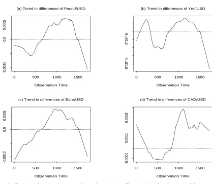
the Epanechnikov kernel is used as the weight function. The estimated local mean functions

are displayed in Figure 3 together with a horizontal line y = 0. Where negative values of

the estimated means correspond to weaker USD periods while positive estimate to strong

USD periods. We see at the current end the USD is stronger than all foreign currencies

except for the CAD, which reflects the current strong dollar policy of the US government.

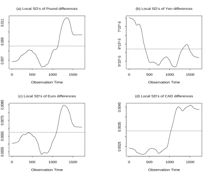
Figure 4 shows the estimated local standard deviations. We can see that the variance

of a difference series also change clearly during this period. The biggest relative change

happens by the CAD, the the ratio between the smallest and biggest values is bigger than

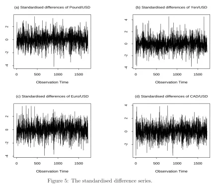
2. The standardized difference series are shown in Figure 5, from which we can see that the

change in the variances is well fitted and removed. Now each single series looks stationary.

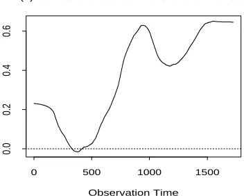
However they are still not jointly stationary, because the cross-correlation matrix changes

very strongly over this period. This is shown in Figure 6, where all of the correlation

coefficients show a clearly increasing pattern. This indicates that the dependence between

the main world economies becomes stronger and stronger in these years. Detailed analysis

shows that the dependence level between the two European currencies was still very high

at the beginning and becomes higher (about 0.8) at the end of the period. The other

correlation coefficients have been very slow at the beginning. Those between Pound and

CAD, and Euro and CAD are even slightly negative at that time. But they increase very

quickly during the observation period until about 0.5 at the current end. At this end the

cross-correlations between CAD and the other currencies seem to begin decreasing slightly

again, because all other currencies become weaker but the CAD is still stronger (cf Figures

1 and 3).

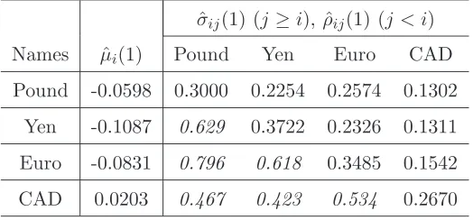
Results obtained following the proposed model are very useful for risk management and

portfolio optimisation. This will be explained briefly in the following. The estimated means,

variances, covariances and correlation coefficients at the current end (with x= 1) for each

currency (standardised for a 100 USD unit to keep them comparable) are shown in Table

1, where the diagonal elements in the second part are the estimated variances, those in

the upper triangular part are the estimated covariances while the estimated correlation

Table 1. ˆµi(1), ˆσij(1) and ˆρij(1) (italic) (for 100 USD).

ˆ

σij(1) (j≥i), ˆρij(1) (j < i)

Names µˆi(1) Pound Yen Euro CAD

Pound -0.0598 0.3000 0.2254 0.2574 0.1302

Yen -0.1087 0.629 0.3722 0.2326 0.1311

Euro -0.0831 0.796 0.618 0.3485 0.1542

CAD 0.0203 0.467 0.423 0.534 0.2670

weakest and the Euro the second weakest currencies. Following the variance (risk) the

Euro is the weakest and the Yen the second weakest currencies. Following both criteria the

CAD is the strongest and the Pound the second strongest currencies. This information is

very useful for decision making, for instance to calculate an optimal portfolio.

7

Concluding remarks

We see that this article provides a good practical model and estimation methods for slowly

changing drifts, variance and correlation coefficients of underlying stochastic process. It is

the first multivariate model in the literature for studying slow change stochastic process;

it develops effect estimation methods and asymptotic theory; and it assesses the effect of

errors in the short term forecasts. Also, any increase in the number of component of the

model does not increase the number of unknown parameters, nor the estimation burden,

hence the model and fitting method are suitable for jointly modelling any number of assets

in practice.

Some important open questions are still there and left for further study. These questions

include extension of the model to allow for autocorrelations, development of significant tests

and the need of robust estimation under asymmetric distribution and possibly outliers in

the data.

The data used in this paper are downloaded from the data releases of the US Federal

Reserve Bank under the address ‘http://www.federalreserve.gov/releases/h10/’. We are

grateful to Prof. Serguei Foss and Dr. George Streftaris, Heriot-Watt University, and Prof.

Winfried Pohlmeier, University of Konstanz, for useful discussions and comments. We are

also grateful to Miss Jiangjiang Yu and Mr Yao-Chih Chen who carried out some empirical

analysis using similar idea in their MSc project under the supervision of the first author.

Appendix:

Proofs of results

Proof of Theorem 2. 1) The results are just special cases of those given in Theorem 1.

2) Note that ˆµi(x) and ˆµj(x) are two linear estimators with the same weights generated

by the local polynomial approach. Let wt denote the weights. We have

ˆ

µi(x) = n

X

t=1

wtzit and µˆj(x) = n

X

t=1

wtzjt.

Note that, for t1 6=t2,zit1 are independent of zit2 andzjt2. Hence

cov (ˆµi(x),µˆj(x)) = cov

n

X

t=1

wtzjt, n

X

t=1

wtzjt

!

=

n

X

t=1

cov (wtzjt, wtzjt)

=

n

X

t=1

w_t2cov (zjt, zjt)

=

n

X

t=1

w_t2σij(xt). (A.1)

Under the conditions of Theorem 2 we have wt= 0 for|x−xt|> hand

σij(xt) =σij(x)[1 +O(h)] =σij(x)[1 +o(1)]

for _|x₋xt| ≤h. Following known results in nonparametric regression it is easy to show

thatPw2_t = (nh)−1_{R[1 +o(1)] (see e.g. Wand and Jones, 1995 and Fan and Gijbels, 1996).}

Hence,

cov (ˆµi(x),µˆj(x)) =

n

X

t=1

= σij(x)[1 +o(1)] n

X

t=1

w2_t

= (nh)−1_Rσ

ij(x)[1 +o(1)]. (A.2)

3) Results in this part can be shown by straightforward calculations. In the following we

will give an indirect proof to show more details. Denote by BS_ˆ

µ(x) andV

S

ˆ

µ(x) respectively

the bias and variance of the estimated portfolio returns. Then it is easy to show that

M SES_ˆ

µ(x) = [B

S

ˆ

µ(x)]

2_+VS

ˆ

µ(x). (A.3)

Following results in part 1) we have

BS_µˆ(x) = E

( _k

X

i=1

Siµˆi(x)

)

−

k

X

i=1

Siµi(x)

= E

( _k

X

i=1

Si[ˆµi(x)−µi(x)]

)

=

( _k

X

i=1

Siµ(p+1)(x)

)

βhp+1

(p+ 1)![1 +o(1)]. (A.4)

Furthermore, following (A.2) we have

V_µˆS(x) = var

( _k

X

i=1

Siµˆi(x)

) = k X i=1 k X j=1

SiSjcov (ˆµi(x),µˆj(x))

=    k X j=1

SiSjσij

  

R

nh[1 +o(1)]. (A.5)

Equation (11) is proved by inserting those in (A.4) and (A.5) into (A.3).

4) Now, note that both TS

1 and T2S are both non-negative. The dominated part of

M SES_ˆ

µ(x) given in (11) is concave inh, provided thatT

S

1 andT2S are both non-zero, which

is minimized by hopt_S given in (14). _⋄

Proof of Theorem 3. Let wit denote the weights for ˆσ2i(1) andwitk,k= 1, ..., n, those

for _|xk−xt| ≤ hi and zero otherwise. Let ξit =zit−µi(xt). We have ξit =σi(xt)˜ǫit and

ξij_t =ξitξjt=σi(xt)˜ǫitσj(xt)˜ǫjt, where ξtij and ˜ǫit are as defined in the context of Theorem

4. Define ηit = ˜ǫ2it−1. Then, for given i,ηit are zero mean i.i.d. errors such that

ξ_it2 =σ2_i(xt) +σi2(xt)ηit, (A.6)

which represents a special nonparametric regression model with independent errors and

scale change, where the scale function turns to be the same as the trend function. A key

point here is thatξit are unobservable. In the following we will show first Theorem 3 holds,

if µi(xt) is known, i.e. if ξit are observable. Define

˜

σ2_i(1) =

n

X

t=1

witξit2, (A.7)

which is a kernel estimator of σ2_i(1) but obtained under the assumption thatξit are

observ-able, i.e. µi(xt) are known. The asymptotic bias and variance of ˜σi2(1) can be obtained

by adapting well known results in nonparametric regression with a scale function. See e.g.

Fan and Gijbels (1995), Efromovich (1999) and Feng (2004). However, for a kernel

estima-tor at the endpoint, the weights are non-symmetric and the first order term in the Taylor

expansion of σ_i2(x) can hence not be cancelled. Denote the bias of ˜σ_i2(1) by B[˜σ_i2(1)]. We

have

B[˜σ_i2(1)] =

n

X

t=1

witE[ξit2]−σ2i(1)

= αi(σi2)′(1)bi[1 +o(1)] (A.8)

as given in 1) of Theorem 3.

The variance of ˜σ_i2(1) is given by

var [˜σ_i2(1)] =

n

X

t=1

w2_itvar (ηit) =

n

X

t=1

w2_itvar (ξ_it2)

.

= γ_ii2(1)

n

X

t=1

w_it2 = (nbi)−1Viγii2(1)[1 +o(1)] (A.9)

as given in 2) of Theorem 3, because Pn_t=1w2

it

.

= (nbi)−1Vi.

We now show that the changes of the asymptotic bias and variance of ˆσ_i2(1) caused by

the error in ˆµi(xt) are both negligible under A4′. Note thatrit=zit−µˆi(xt) and

r_it2 = z_it2 ₋2zitµˆi(xt) + ˆµ2i(xt)

= ξ_it2 + 2ξit∆it+ ∆2it, (A.10)

where ∆it =µi(xt)−µˆi(xt) is the estimation error in ˆµi(xt), for which we have

∆it=O(h2i) +Op[(nhi)−1/2]. (A.11)

Following (A.10) we have

E[ˆσ_i2(1)₋σ_i2(1)] =B[˜σ_i2(1)] +

n

X

t=1

wit[2E(ξit∆it) +E(∆2it)]. (A.12)

Furthermore,

E(ξit∆it) = E

"

ξit n

X

k=1

witkzik−µi(xt)

!#

= E

"

ξit n

X

k=1

witk[ξik+µi(xk)]−µi(xt)

!#

= wittσ2i(xt) =O[(nhi)−1], (A.13)

since ξit are i.i.d. with E(ξit) = 0 andE(ξ_it2) =σ_i2(xt), and

E(∆2_it) = MSE[ˆµi(xt)]

= O[h4_i + (nhi)−1]. (A.14)

Condition A4′ _{means that h}4

i = o(n−2/3), (nhi)−1 = o(n−2/3) and bi > O(n−2/3). This

ensures that O[h4_i + (nhi)−1] =o(bi) =o{B[˜σ2i(1)]}. Observe that

P

wit= 1 we obtain

E[ˆσ2_i(1)₋σ2_i(1)] = B[˜σ2_i(1)] +O[h4_i + (nhi)−1]

= B[˜σ2_i(1)][1 +o(1)]. (A.15)

Now we will analyze the effect of the error in ˆµi(xt) on var (ˆσi(1)). Note first that

Although cov (z_it2

1, z

2

it2) = cov (ξ

2

it1, ξ

2

it2) = 0 for t16=t2, but cov (r

2

it1, r

2

it2)6= 0. Following

the first equation in (A.10) we have

cov (r_it2₁, r_it2₂) = cov (z_it2_{1 −}2zit1µˆi(xt1) + ˆµ

2

i(xt1), z

2

it2−2zit2µˆi(xt2) + ˆµ

2

i(xt2))

= C1+C2+C3+C4+C5+C6+C7+C8+C9,

where C1 = cov (zit21, z

2

it2) = 0,C2 =−2cov (z

2

it1, zit2µˆi(xt2)), C3 = cov (z

2

it1,µˆ

2

i(xt2)),

C4=−2cov (zit1µˆi(xt1), z

2

it2), C5 = 4cov (zit1µˆi(xt1), zit2µˆi(xt2)),

C6 =−2cov (zit1µˆi(xt1),µˆ

2

i(xt2)), C7= cov (ˆµ

2

i(xt1), z

2

it2),

C8=−2cov (ˆµ2i(xt1), zit2µˆi(xt2)), C9 = cov (ˆµ

2

i(xt1),µˆ

2

i(xt2)).

It can be shown that C2 =C4 =C5 = 0. This will be shown for C2.

C2 = −2cov zit21, zit2

n

X

k=1

wit2kzik

!

= ₋2

n

X

k=1

wit2kcov (z

2

it1, zit2zik) = 0, (A.17)

because zit are i.i.d.,t16=t2 and hence cov (z2it1, zit2zik) = 0,for all k. Hence,

cov (r_it2₁, r2_it2) =C3+C6+C7+C8+C9. (A.18)

For C3 we have

C3 = cov zit21,

n X k=1 n X l=1

wit2kwit2lzikzil

! = n X k=1 n X l=1

wit2kwit2lcov (z

2

it1, zikzil)

= w_it2_2t1var (z_it2₁) (A.19)

due to the term with k = l= t1, because all other covariances are equal to zero. Similar

calculations lead to

C6 =−2wit1t1w

2

it2t1var (z

2

it1), C7=w

2

it1t2var (z

2

it2),

C8=−2w2it1t2wit2t2var (z

2

it2), C9 =

n

X

k=1

Observe the properties of the weights it is easy to see that C3 = O(C7) = O[(nhi)−2],

C6 =O(C8) =O(C9) =O[(nhi)−3] =o(C3). That is

cov (r_it2₁, r2_it2)=. w2_it2t1var (z_it2₁) +w_it2_1t2var (z_it2₂) =O[(nhi)−2]. (A.20)

We see cov (r2

it1, r

2

it2) =o(n

−1_{), ifh}

i> O(n−1/2), which is implied by A4′. Hence we have

var [ˆσ_i2(1)] = var

" _n X

t=1

witrit2

#

=

n

X

t=1

w2_itvar (r_it2) +

n

X

t1=1

n

X

t

2=1

t₂6=t₁

wit1wit2cov (r

2

it1, r

2

it2)

.

=

n

X

t=1

w2_itvar (r_it2)

.

=

n

X

t=1

w2_itvar (ξ_it2) = var [˜σ2_i(1)]. (A.21)

Theorem 3 is proved. _⋄

Proof of Theorem 4. Note that the biases are of the same order as in Theorem 3. And

the variances and convariances are of the same order as the variances in Theorem 3. The

estimation errors in ˆµi(xt) are also negligible under A4′. In the following proof the residuals

rit will hence be simply replaced byξit.

By extending the ideas described at the beginning of the proof of Theorem 3 we can

obtain

ξ_tij =σij(xt) +σi(xt)σj(xt)ζtij, (A.22)

where ζ_tij = ˜ǫitǫ˜jt−ρij(xt) are i.i.d. zero mean random variables. This is again a special

nonparametric regression model with i.i.d. errors and a scale function, where the trend

is the corresponding covariance function. Of course (A.6) is a special case of (A.22) with

i=j.

1) As mentioned before, the bias of ˆσij(1) is not affected by the scale function and is the

same as in common nonparametric regression. The proof of this part is hence omitted.

by Wr(u) defined in Theorem 4 and the bandwidthb. We have

ˆ

σij(1) =

n

X

t=1

wtξijt

and

cov (ˆσij(1),σˆlm(1)) =

n

X

t1=1

n

X

t2=1

wt1wt2cov (ξ

ij t1, ξ

lm t2 )

=

n

X

t=1

w_t2cov (ξij_t , ξ_tlm)

= γij, lm n

X

t=1

w_t2 (A.23)

following the definition before, since cov (ξ_tij

1, ξ

lm

t2 ) = 0 for t16=t2. Furthermore we have

cov (ˆσij(1),σˆlm(1)) =V γij, lm(nb)−1[1 +o(1)], (A.24)

becausePn_t=1w2_t =V(nb)−1_{[1 +o(1)], whereV =}R0

−1(Wr(u))2duas defined in Theorem 4.

3) Denote byB the bias. It is easy to show that, for given i, j, l, m,

E_{[ˆσij(1)−σij(1)][ˆσlm(1)−σlm(1)]} = B[ˆσij(1)]B[ˆσlm(1)] + cov [ˆσij(1),σˆlm(1)](A.25).

Using results in 1) we have

B[ˆσij(1)]B[ˆσlm(1)] =α2σ′ij(1)σ′lm(1)b2[1 +o(1)]. (A.26)

Insert these results and those in 2) into (24) we obtain the results in 3) of Theorem 4.

4) Results in this part follow from those in 3) directly.

Proof of Theorem 5. 1) Under the smoothness assumption onµi we have µi(xn+t) =

µi(1) +O(T n−1) for any t≤T. Following (32) and (33) we have

E[ ˆY_i(n+T)−E(Y_i(n+T)|Yin)]2 = E[Tµˆi(1)− T

X

t=1

µi(xn+t)]2

= T2E_{[ˆµi(1)−µi(1)] +O(T n−1)]}2. (A.27)

Note that ˆµi(1)−µi(1) =O(h(ip+1)) +Op[(nhi)−1/2]. The conditionT2(nhi)−1 →0 results

in T =o(nh1_i/2) andT n−1_=o[n−1/2_h1/2

i ] =o[ˆµi(1)−µi(1)]. Hence,

E[ ˆYi(n+T)−E(Yi(n+T)|Yin)]2 =. T2E[ˆµi(1)−µi(1)]2

Furthermore, A5 ensures that T2M SE[ˆµi(1)]→0, i.e. ˆYi(n+T) is consistent.

2) Similarly, under the conditions of Theorem 5 it can be shown that

E[ ˆP_nS_{+T −}E(P_nS_+T|Yn)]2 =. T2E

( _k

X

i=1

Si[ˆµi(1)−µi(1)]

)2

= T2M SES_ˆ

µ, (A.29)

T2_{M SE}S

ˆ

µ→0 under A5 and ˆP

S

n+T is consistent. ⋄

Proof of Theorem 6. 1) Note that ˆσi(1) =

q

ˆ

σ2

i(1). Based on Taylor expension of

random variables it can be shown that

M SE[ˆσi(1)] =O(M SE[ˆσ2i(1)]). (A.30)

Analogously to the analysis in 1) of the proof of Theorem 5 we have σ2

i(xn+t) = σi(1) +

O(T n−1_{) for any t≤T and}

E[√Tσˆi(1)−SDT]2 = E

  

√

Tσˆi(1)−

v u u t " _T X t=1 σ2

i(xn+t)

#_



2

.

= En√Thˆσi(1)−σi(1) +O(T1/2n−1/2)

io2

.

= T_·E[ˆσi(1)−σi(1)]2

= O(T _·M SE[ˆσ_i2(1)]). (A.31)

Condition A5′ _{ensures thatT}1/2_n−1/2 _=o[ˆσ

i(1)−σi(1)],T·M SE[ˆσ2i(1)]→0 and

√ Tˆσi(1)

is a consistent estimator of SDT.

2) Similarly, it can be shown that

M SE

q

S′_Σˆ_(1)S

.

=M SES_ˆ

Σ(1), (A.32)

E

q

T S′_Σ(1)ˆ _S−SDS

T

2

.

= T _·M SE

q

S′_Σˆ_(1)S

= T _·M SES_ˆ

Σ(1). (A.33)

AndT _·M SES

ˆ

Σ(1)→0 under A5

′ _{so that}

q

REFERENCES

A¨ıt-Sahalia, Y. (1996) Nonparametric pricing of interest rate derivative securities,

Econo-metrica,64,527–560.

Beran, J. and Y. Feng (2002) SEMIFAR models – a semiparametric approach to modelling

trends, long-range dependence and nonstationarity. Comptat. Statist. & Data Anal.,40,

393–419.

Beran, J. and Ocker, D. (1999) SEMIFAR forecasts, with applications to foreign exchange

rates. J. Statistical Planning and Inference,80, 137–153.

Bollerslev, T., R. F. Engle and J. Wooldridge (1988) A capital asset-pricingmodel with

time-varying covariances. Journal of Political Economy, 96, 116131.

Cs¨org¨o, S. and J. Mielniczuk (1995) Nonparametric regression under long-range dependent

normal errors. Annals of Statistics,23, 1000–1014.

Dahlhaus, R. (1997) Fitting time series models to nonstationary processes. Annals of

Statistics,25, 1–37.

Dahlhaus, R. (2000) A likelihood approximation for locally stationary processes. Annals of

Statistics,28, 1762–1794.

Efromovich, S. (1999)Nonparametric curve estimation: Methods, Theory, and Applications.

New York: Springer.

Engle, R.F. (1982) Autoregressive Conditional Heteroscedasticity with Estimates of the

Variance of UK Inflation. Econometrica,50, 987-1008

Engle, R. (2002) Dynamic conditional correlation: A simple class of multivariate generalized

autoregressive conditional heteroskedasticity models. Journal of Business and Economic

Statistics,20, 339–350.

Fan, J. and I. Gijbels (1995) Data-driven bandwidth selection in local polynomial fitting:

Variable bandwidth and spatial adaptation. J. Roy. Statist. Soc. Ser. B,57,371–394.

Fan, J. and Q. Yao (1998) Efficient estimation of conditional variance functions in stochastic

Feng, Y. (2004) Simultaneously modelling conditional heteroskedasticity and scale change.

Econometric Theory,20,563–596.

Gasser, T., A. Kneip and W. K¨ohler (1991) A flexible and fast method for automatic

smoothing. J. Amer. Statist. Assoc.,86, 643–652.

Gordon, A.H. (1991) Global warming as a manifestation of a random walk. Journal of

Climate,4, 589-597.

H¨ardle, W., A.B. Tsybakov and L. Yang (1998) Nonparametric vector autoregression. J.

Statist. Plann. Infer., 68,221–245.

H¨ardle, W., H. Herwatz and V. Spokoiny (2003) Time inhomogeneous multiple volatility

modelling. J. Financial Econometrics,1,55–99.

Hart, J. D. (1991) Kernel regression estimation with time series errors. J. Roy. Statist.

Soc. Ser. B,53, 173–187.

Harvey, A. (1989) Forecasting structural time series models and the Kalman filter.

Cam-bridge: Cambridge University Press.

Harvey, A., Ruiz, E. and N. Shephard (1994) Multivariate stochastic variance models.

Review of Economic Studies,61, 247–264.

Herzel, S., C. Starica and R. Tutuncu (2006) A non-stationary multivariate model for

financial returns. Forthcoming in Statistics for dependent data, Ed. Patrice Bertail, and

P. Doukhan, Springer.

K¨arner, O. (2002) On nonstationarity and antipersistency in global temperature series.

Journal of Geophysical Research,107, doi: 10.1029/2001JD002024.

Kijima, M. (2002)Stochastic Processes with Applications to Finance, Cambridge: Chapman

and Hall.

Lov´asz, L. (1993) Random Walks on Graphs: A Survey,Mathematical Studies,2, 1–46.

Neigel, J. E. and J.C. Avise (1993) Application of a random walk model to geographic

Ruppert, D. and M.P. Wand (1994) Multivariate locally weighted least squares regression.

Annals of Statistics,22, 1346–1370.

Wand, M.P. and M.C. Jones (1995) Kernel Smoothing, London: Chapman & Hall.

Weiss, G.H. (1994) Aspects and Applications of the Random Walk, Amsterdam: North

Holland Press.

Wu, W. and M. Pourahmadi (2003) Nonparametric estimation of large covariance matrices

of longitudinal data. Biometrika, 90, 831–844.

0 500 1000 1500

1.4

1.5

1.6

1.7

1.8

1.9

(a) Exchange rates between Pound/USD

Observation Time

0 500 1000 1500

0.0075

0.0085

0.0095

(b) Exchange rates between Yen/USD

Observation Time

0 500 1000 1500

0.9

1.0

1.1

1.2

1.3

(c) Exchange rates between Euro/USD

Observation Time

0 500 1000 1500

0.65

0.75

0.85

(d) Exchange rates between CAD/USD

Observation Time

0 500 1000 1500

-0.04

-0.02

0.0

0.02

(a) Differences of Pound/USD

Observation Time

0 500 1000 1500

-0.0003

-0.0001

0.0001

(b) Differences of Yen/USD

Observation Time

0 500 1000 1500

-0.02

0.0

0.01

(c) Differences of Euro/USD

Observation Time

0 500 1000 1500

-0.010

0.0

0.010

(d) Differences of CAD/USD

Observation Time

0 500 1000 1500

-0.0010

0.0

0.0005

(a) Trend in differences of Pound/USD

Observation Time

0 500 1000 1500

-8*10^-6

-2*10^-6

(b) Trend in differences of Yen/USD

Observation Time

0 500 1000 1500

-0.0010

0.0

0.0005

(c) Trend in differences of Euro/USD

Observation Time

0 500 1000 1500

-0.0001

0.0001

0.0003

(d) Trend in differences of CAD/USD

Observation Time

Figure 3: Estimated mean functions from the series in Figure 2 (with a horizontal line at

0 500 1000 1500

0.007

0.009

0.011

(a) Local SD’s of Pound differences

Observation Time

0 500 1000 1500

5*10^-5

6*10^-5

7*10^-5

(b) Local SD’s of Yen differences

Observation Time

0 500 1000 1500

0.0055

0.0065

0.0075

0.0085

(c) Local SD’s of Euro differences

Observation Time

0 500 1000 1500

0.0025

0.0035

0.0045

(d) Local SD’s of CAD differences

Observation Time

0 500 1000 1500

-4

-2

0

2

(a) Standardised differences of Pound/USD

Observation Time

0 500 1000 1500

-4

-2

0

2

4

(b) Standardised differences of Yen/USD

Observation Time

0 500 1000 1500

-4

-2

0

2

(c) Standardised differences of Euro/USD

Observation Time

0 500 1000 1500

-2

0

2

4

(d) Standardised differences of CAD/USD

Observation Time

0 500 1000 1500

0.1

0.3

0.5

(a) Correlations between Pound/Yen differences

Observation Time

0 500 1000 1500

0.0

0.2

0.4

0.6

(b) Correlations between Yen/Euro differences

Observation Time

0 500 1000 1500

0.55

0.65

0.75

(c) Correlations between Pound/Euro differences

Observation Time

0 500 1000 1500

0.1

0.2

0.3

0.4

0.5

(d) Correlations between Yen/CAD differences

Observation Time

0 500 1000 1500

0.0

0.2

0.4

(e) Correlations between Pound/CAD differences

Observation Time

0 500 1000 1500

0.0

0.2

0.4

0.6

(f) Correlations between Euro/CAD differences

Observation Time